Statistics of Sliding on Periodic and Atomically Flat Surfaces

Among the so-called analytical models of friction, the most popular and widely used one, the Prandtl-Tomlinson model in one and two dimensions is considered here to numerically describe the sliding of the tip within an atomic force microscope over a periodic and atomically flat surface. Because in these PT-models, the Newtonian equations of motion for the AFM-tip are Langevin-type coupled stochastic differential equations the resulting friction and reaction forces must be statistically correctly determined and interpreted. For this, it is firstly shown that the friction and reaction forces as averages of the time-resolved ones over the sliding part, are normally (Gaussian) distributed. Then based on this, an efficient numerical scheme is developed and implemented to accurately estimate the means and standard deviations of friction and reaction forces without performing too many repetitions for the same sliding experiments. The used corrugation potential is the simplest one obtained from the Fourier series expansion of the two-dimensional (2D) periodic potential, e.g., for an fcc(111) surface, which permits sliding on both commensurate and incommensurate paths. In this manner, it is proven that the PT-models predict both frictional regimes, namely the structural superlubricity and stick-slip along (in)commensurate sliding paths, if the ratio of mean corrugation and elastic energies is properly set.

1 Introduction

Frictional experiments in an atomic force microscope can be straightforwardly simulated by using either molecular dynamics (MD) or ab-initio (first-principles) methods, see for example, Refs. (Kobayashi et al., 2016; Wolloch et al., 2015). From a computational point of view, however, these numerical calculations are extremely demanding and time consuming. Therefore, the so-called one-dimensional (1D) and two-dimensional (2D) analytical models of friction, such as the Prandtl-Tomlinson and Frenkel-Kontorova models, (Dong et al., 2011) are still remaining to be highly efficient alternatives to the atomistic models and hence very popular because of their simplicity with which they are capturing the main undergoing mechanisms within nanotribological AFM-experiments. (Pawlak et al., 2016)

The Prandtl-Tomlinson model (PT-model), in its original formulation, (Prandtl, 1928) was introduced by Prandtl while developing a kinetic theory of solids assuming a periodic interaction between the bodies. Curiously, in the other paper ascribed to the PT-model, (Tomlinson, 1929) Tomlinson was not dealing at all with these concepts, since he was outlining a molecular theory of friction based on the findings by Lennard-Jones. Despite this historical inaccuracy, (Popov and Gray, 2012) within a 1D or 2D PT-model, one can clearly distinguish between various frictional regimes by considering a single parameter, namely the ratio between the average interaction and elastic energies. (Socoliuc et al., 2004)

Traditionally, if the coefficient-of-friction (CoF) observed for a tribological system is less than or equal to 0.01 that system is said to evolve within a superlubric frictional regime. (Martin and Erdemir, 2018) Superlubricity was predicted theoretically in 1990 by Hirano and Shinjo, (Hirano and Shinjo, 1990) and its occurrence was shown experimentally 1 year later. (Hirano et al., 1991) Nowadays, beyond this structural superlubricity discovered in the nineties as caused by the incommensurability of interacting surfaces, one speaks also about thermolubricity (Krylov et al., 2005) and chemolubricity (Erdemir and Martin, 2007) which are two other forms of superlubricity caused by the temperature acting as lubricant and due to chemistry, respectively. For further information on superlubricity, the reader is recommended to consult the excellent reviews in the newest book edited by J.-M. Martin and A. Erdemir. (Erdemir et al., 2021)

In this contribution, the structural superlubricity will be addressed numerically by using the most popular and hence widely applied analytical model of friction, namely the PT-model in one-dimension and two-dimensions, in its well-known form from the kinetic theory of solids and solid mechanics, see Section 2. For this, the periodic corrugation of interest is explicitly derived in Section 4 and directly introduced into the corresponding 1D/2D PT-model. Since the resulting Newtonian equations of motion are forming a set of stochastic differential equations (SDEs), they are solved numerically by applying an adequate fourth-order Runge-Kutta method as presented in Section 3. Due to the randomness of the thermally induced force mimicking the impact of temperature on the sliding, both frictional regimes, either stick-slip or superlubric, must be statistically evaluated and interpreted, for example, in terms of distributions as shown in Secion 5. Beyond the development of a statistically proper numerical scheme for comparing the calculated frictional performance along various paths on periodic atomic surfaces, the ultimate goal of this contribution is to elucidate in which circumstances, i.e., range of various parameters such as materials, elastic coupling of AFM-tip to the drive, sliding velocity or absolute temperature, one could detect the superlubric frictional regime with high accuracy, see Section 6.

2 Prandtl-Tomlinson Models

In an atomic force microscope, the movement of the tip on a corrugated surface of a substrate in dry contact conditions is described within the kinetic theory of solids by the Langevin equation of motion, (Filippov et al., 2010)

$m\frac{d^2\mathit{r}(t)}{d{t}^2}+m\gamma \frac{d\mathit{r}(t)}{dt}+\nabla V(\mathit{r},t)=\mathit{\zeta }(t),(1)$

with r(t) being the time-dependent position of the AFM-tip of mass m and γ is characterizing the damping proportional to the velocity of the AFM-tip. Here the first force on the left-hand side is that which accelerates the AFM-tip, the second one acts against the former and it is proportional to the velocity of the AFM-tip, whereas the last, third force on the left-hand side is due to the interaction of the AFM-tip with the surface and with the drive.

If the total potential energy consists of the time independent corrugation potential U(r) and the elastic potential of the tip-drive subsystem, respectively, then

$V(\mathit{r},t)=U(\mathit{r})+\frac{1}{2}{k}_c{\left({\mathit{v}}_{s}t-\mathit{r}\right)}^2,(2)$

where k_c stands for the effective stiffness of the linear coupling (e.g., via spring) between the AFM-tip and drive. Note that the drive is supposed to move with a constant sliding velocity v_s, such that

${\mathit{v}}_s=v_s\left(\mathit{i}\cos \mathrm{\Phi }+\mathit{j}\sin \mathrm{\Phi }\right),(3)$

with Φ defining the orientation of the sliding path with respect to the Cartesian x-axis, whereas i and j being the in-plane unity vectors along the Cartesian axes. The relative direction of v_s also sets the commensurability/incommensurability of the sliding path versus the periodicity of corrugation U(r), for more details see Secion 4 below. For example, for a 2D corrugation one can consider the same functional form as for the 1D, such that the latter 1D corrugation provides a periodic atomic chain according to Φ, whereas in the 2D case it represents the simplest 2D periodic potential corresponding to the crystalline orientation of substrate’s surface.

In Eq. 1, a normal (Gaussian) distribution is assumed for the amplitude of the thermal-noise-induced random force ζ(t), thus for its ensemble averaged auto-correlation function holds that

$⟨\zeta (t)\zeta (t^{\prime })⟩=2m\gamma k_{B}T\delta \left(t-t^{\prime }\right),(4)$

where δ denotes the Dirac delta-function, k_B is the Boltzmann constant and T stands for the absolute temperature, and its random orientation is given by

$\mathit{\zeta }(t)=\zeta (t)\left(\mathit{i}\cos \theta +\mathit{j}\sin \theta \right)(5)$

with θ being a uniformly distributed random angle.

3 Runge-Kutta Methods

In the following, some details on the implementation are given, which can be directly used for a 1D PT-model as well as for a 2D PT-model where ξ(t) is measured along the sliding path. In this case, the second-order stochastic differential equation in Eq. 1 is equivalent to a system of two coupled first-order differential equations,

$\left\{\begin{array}{cc}\frac{d\xi (t)}{dt}\hfill & =v(t)\hfill \\ \hfill & \hfill \\ \frac{dv(t)}{dt}\hfill & =\frac{1}{m}\zeta (t)-\gamma v(t)-\frac{1}{m}\frac{\partial V(\xi ,t)}{\partial \xi }\hfill \end{array}\right.,(6)$

which, once numerically solved, yields simultaneously the position ξ(t) and velocity v(t) of the AFM-tip along the sliding path for ∀t ≥ t₀, if the initial position ξ₀ and velocity v₀ of the AFM-tip are both known at the starting time t₀, i.e.,

$\left\{\begin{array}{cc}\xi (t_0)\hfill & ={\xi }_0\hfill \\ \hfill & \hfill \\ v(t_0)\hfill & =v_0\hfill \end{array}\right..(7)$

The Runge-Kutta (RK) methods for solving differential equations numerically were independently developed by Runge (Runge, 1895) and Kutta (Kutta, 1901) more than a century ago. During their long history, (Butcher and Wanner, 1996) they were continuously improved, (Kalogiratou et al., 2014) such that also RK-methods exist for solving SDEs, one of which will be here applied as follows. The fourth-order Runge-Kutta method applied for the coupled SDEs in Eq. 6, i.e., when T > 0, means that one knowing ξ_n = ξ(t_n) and v_n = v(t_n) for t_n = n Δt (∀n = 0, 1, 2, …), computes for i = 1, 2, 3, 4

$\left\{\begin{array}{cc}{t}_i\hfill & =t_n+\sum _{j=1}^{i-1}{a}_{ij}\mathrm{\Delta }t\hfill \\ \hfill & \hfill \\ {\xi }_i\hfill & ={\xi }_n+\sum _{j=1}^{i-1}{a}_{ij}{k}_{i,\xi }\hfill \\ \hfill & \hfill \\ v_i\hfill & =v_n+\sum _{j=1}^{i-1}{a}_{ij}{k}_{i,v}\hfill \\ \hfill & \hfill \\ w_i\hfill & =G_i\sqrt{\frac{q_i}{\mathrm{\Delta }t}W}\hfill \end{array}\right.\Rightarrow \left\{\begin{array}{cc}{k}_{i,\xi }\hfill & =\mathrm{\Delta }t{v}_i\hfill \\ \hfill & \hfill \\ k_{i,v}\hfill & =-\mathrm{\Delta }t\left[\gamma v_i+\frac{1}{m}\frac{\partial V({\xi }_i,t_i)}{\partial \xi }\right]+\mathrm{\Delta }t\frac{w_i}{m}\hfill \end{array}\right.,$

to finally get

$\left\{\begin{array}{c}{\xi }_{n+1}={\xi }_n+b_1{k}_{1,\xi }+b_2{k}_{2,\xi }+b_3{k}_{3,\xi }+b_4{k}_{4,\xi }\hfill \\ \hfill \\ v_{n+1}=v_n+b_1{k}_{1,v}+b_2{k}_{2,v}+b_3{k}_{3,v}+b_4{k}_{4,v}\hfill \end{array}\right.+\mathcal{O}(\mathrm{\Delta }t{}^4),\forall n=\mathrm{0,1,2},\dots ,$

where all the involved real-valued coefficients as derived in Ref. (Kasdin, 1995), G_i (i = 1, …, 4) are Gaussian random numbers and W = 2mγ k_BT in accordance with Eq. 5. Due to this latter randomness at finite absolute temperature, Eq. 6 admits not only a single exact solution, but a set of differently valued solutions which, however, are all statistically equivalent down to T = 1 mK–as we found. On the other hand, in accordance with Eq. 5, the thermal-noise-induced random force ζ(t) is vanishing at absolute zero temperature, since W = 0 when T = 0 K, and hence the first-order SDE in Eq. 6 turns at T = 0 K into an ordinary differential equation (ODE) and therefore the ‘classical’ fourth-order Runge-Kutta method for ODEs can be immediately applied. Formally, this means that one considers the former expressions with w_i = 0 (i = 1, …, 4) and the following tableaux of Runge-Kutta coefficients, (Press et al., 2007)

$\begin{array}{cccc}\hfill a_{21}\hfill & \hfill \hfill & \hfill \hfill & \hfill \hfill \\ \hfill a_{31}\hfill & \hfill a_{32}\hfill & \hfill \hfill & \hfill \hfill \\ \hfill a_{41}\hfill & \hfill a_{42}\hfill & \hfill a_{43}\hfill & \hfill \hfill \\ \hfill b_1\hfill & \hfill b_2\hfill & \hfill b_3\hfill & \hfill b_4\hfill \end{array}=\begin{array}{cccc}\hfill \frac{1}{2}\hfill & \hfill \hfill & \hfill \hfill & \hfill \hfill \\ \hfill 0\hfill & \hfill \frac{1}{2}\hfill & \hfill \hfill & \hfill \hfill \\ \hfill 0\hfill & \hfill 0\hfill & \hfill 1\hfill & \hfill \hfill \\ \hfill \frac{1}{6}\hfill & \hfill \frac{1}{3}\hfill & \hfill \frac{1}{3}\hfill & \hfill \frac{1}{6}\hfill \end{array}.(8)$

4 Corrugation Potential and Frictional Regimes

In the following, the corrugation potential of fcc(111)–the conceptual model considered in this contribution–is derived from the Fourier series expansion of the 2D translational invariant potential. For this, consider the 2D primitive lattice vectors for an fcc(111) crystalline surface as being

$\left\{\begin{array}{cc}{\mathit{a}}_1\hfill & =a\left(\mathrm{1,0}\right)\hfill \\ \hfill & \hfill \\ {\mathit{a}}_2\hfill & =a\left(\frac{1}{2},\frac{\sqrt{3}}{2}\right)\hfill \end{array}\right.,(9)$

with $a=a_{\text{fcc}}/\sqrt{2}$ denoting the 2D lattice constant, where a_fcc is the lattice constant of the 3D fcc crystal. Accordingly, the 2D translation vectors are given by T_n = n₁a₁ + n₂a₂, with $n_1,n_2\in \mathbb{Z}$ and correspond to a 2D hexagonal Bravais lattice with an angle γ = π/3 rad between a₁ and a₂, since   cos γ = a₁ ⋅a₂ = 1/2. The 2D reciprocal primitive vectors b_j (j = 1, 2), on the other hand, are directly obtained from Laue’s equations, a_i ⋅b_j = 2πδ_ij (i, j = 1, 2), where δ_ij is the Kronecker symbol, such that by using Eq. 9,

$\left\{\begin{array}{cc}{\mathit{b}}_1\hfill & =\frac{2\pi }{a}\left(1,-\frac{1}{\sqrt{3}}\right)\hfill \\ \hfill & \hfill \\ {\mathit{b}}_2\hfill & =\frac{2\pi }{a}\left(0,\frac{2}{\sqrt{3}}\right)\hfill \end{array}\right.(10)$

and hence the corresponding translation vector within the 2D reciprocal space reads K_m = m₁b₁ + m₂b₂ ($m_1,m_2\in \mathbb{Z}$).

Now, from the Fourier series expansion of the 2D periodic potential U(r) = U(r + T_n),

$U(\mathit{r})=\sum _{{\mathit{K}}_m}{U}_{{\mathit{K}}_m}\exp (i{\mathit{K}}_m\mathit{r}),$

written for $\mathit{r}=x\mathit{i}+y\mathit{j}=\xi \left(\mathit{i}\cos \phi +\mathit{j}\sin \phi \right)$ and by also using Eq. 10, the real part of the “first” Fourier expansion terms

$\frac{\mathrm{R}\mathrm{e} {\left.U(\mathit{r})\right|}_{\pm 10}}{U_{\pm 10}}+\frac{\mathrm{R}\mathrm{e} {\left.U(\mathit{r})\right|}_{0\pm 1}}{U_{0\pm 1}}=\cos \left[\frac{2\pi }{a}\xi \left(\cos \phi -\frac{\sin \phi }{\sqrt{3}}\right)\right]+\cos \left(\frac{2\pi }{a}\xi \frac{2\sin \phi }{\sqrt{3}}\right),$

can be immediately considered as a proper model of the interaction potential between the AFM-tip and fcc(111) surface, e.g., by assuming for sake of simplicity that U_±10 = U_0±1 = U₀₀. In this manner, one could have any desired sinusoidal corrugation as defined by φ, for example,

$U(\xi )=-\frac{U_0}{2}\cos \left[\frac{2\pi }{a}\xi \left(\cos \phi -\frac{\sin \phi }{\sqrt{3}}\right)\right],(11)$

providing the temperature independent force acting on the AFM-tip in the form of

$\frac{\partial V(\xi ,t)}{\partial \xi }=\frac{\pi }{a}{U}_0\left(\cos \phi -\frac{\sin \phi }{\sqrt{3}}\right)\sin \left[\frac{2\pi }{a}\xi \left(\cos \phi -\frac{\sin \phi }{\sqrt{3}}\right)\right]-k_c\left(v_{s}t-\xi \right).(12)$

Indeed, when φ = 0, the most applied and simplest sinusoidal corrugation of period equal to the lattice constant a results,

${\left.U(\xi )\right|}_{\phi =0}=-\frac{U_0}{2}\cos \left(\frac{2\pi }{a}\xi \right)\mathrm{a}\mathrm{n}\mathrm{d}{\left.\frac{\partial V(\xi ,t)}{\partial \xi }\right|}_{\phi =0}=\frac{\pi }{a}{U}_0\sin \left(\frac{2\pi }{a}\xi \right)-k_c\left(v_{s}t-\xi \right).(13)$

Considering in these latter expressions ξ = Γ cos Φ, via Φ one can easily select any commensurate/incommensurate path for sliding, by letting Φ either to show or not to point along a high-symmetry direction on fcc(111), for example, when Φ = 0 or Φ = π/12 = 15^◦.

The values for all the parameters entering Eqs 1–4, 13 are from Ref. (Dong et al., 2011), e.g., a = 2.88 Å, and U₀ = 0.6 eV, and hence correspond to fcc Au(111). However, for the large-parametric study presented in Seciton 6, both U₀ and k_c were continuously varied to determine the impact of the substrate’s material and that of the coupling strength on the friction. When k_c is kept unaltered, then its constant value is set to 1 N/m. As already mentioned, it turned out that independently of the sliding path, whether it is commensurate or incommensurate, the realization of a normal stick-slip as illustrated in Figure 1, or a superlubric frictional regime provided by Figure 2 indeed is only depending on a single quantity,

$\eta =\frac{{\pi }^2{U}_0}{\frac{k_c{a}^2}{2}}(14)$

namely on the ratio between the mean interaction energy of the AFM-tip with the surface and the elastic energy of spring coupling the AFM-tip to the drive, (Socoliuc et al., 2004) see also Section 6.

FIGURE 1

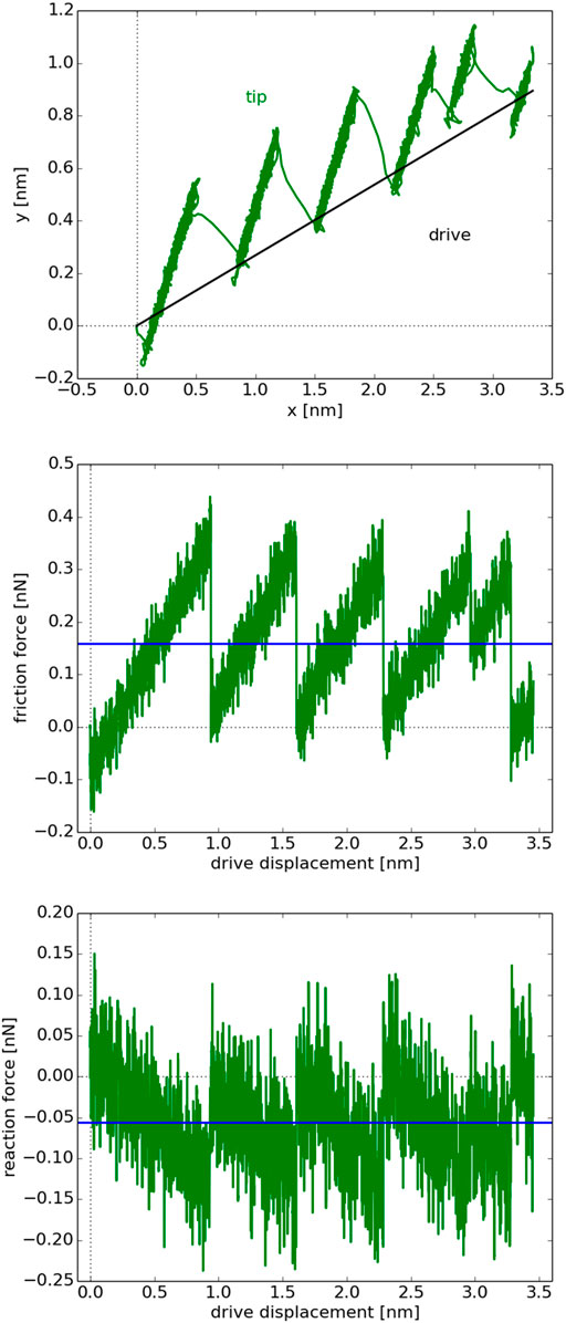
FIGURE 1. Stick-slip movement of the AFM-tip at RT of 300 K along an incommensurate sliding path Φ = 15 deg for an η set accordingly, when U₀ is kept constant and k_c is adjusted, recall Eqs 3, 14. The trajectories of drive (black) and AFM-tip (green) are shown in the top panel, whereas the friction and reaction forces (green) at each position of the drive are given in the middle and bottom panels together with their means (blue) over the entire sliding path.

FIGURE 2

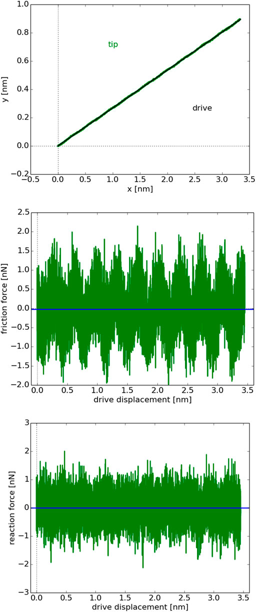
FIGURE 2. As in Figure 1, for an η-value leading to a superlubric sliding of the AFM-tip on an fcc(111) substrate.

5 Statistics of Forces

From Eq. 13 it becomes immediately clear that the average of the lateral force $F\left(t\right)=k_c\left[v_{s}t-\xi \left(t\right)\right]$ taken over the sliding time or distance, for example,

$F_i=\frac{1}{N_t^{\left(i\right)}}\sum _{j=1}^{N_t^{\left(i\right)}}F\left(t_j\right)(15)$

is a proper measure for the friction force and completely in accordance with the experimental practice. (Schwarz and Hölscher, 2016; Peng et al., 2020) Note, however, that accordingly the calculated friction force could be either positive or negative valued, depending on whether the drive is more times in advance with respect to the AFM-tip or the other way around during the entire sliding period. In this Eq. 15, $N_t^{\left(i\right)}$ denotes the number of time moments considered during the ith repetition of the same sliding experiments, normally, a couple of thousands time moments up to 10⁴. Here and in the following for producing reference data, at a non-vanishing absolute temperature between 1 mK and the room-temperature (RT) of 300 K, for example, the mean of a force

${⟨\langle F\rangle ⟩}_n=\frac{1}{n}\sum _{i=1}^n{F}_i(16)$

either frictional or reaction one (the latter only within the 2D PT-model), and its standard deviation

${\sigma }_n=\sqrt{\frac{1}{n}\sum _{i=1}^n{\left(F_i-{⟨\langle F\rangle ⟩}_n\right)}^2}(17)$

are both calculated using numerical results from n = 10⁴ times repeated “identical” sliding experiments, since it is assumed that after such an amount of repetitions ${⟨\langle F\rangle ⟩}_n$ and σ_n are fairly approximating their exact values

$\left\{\begin{array}{cc}⟨\langle F\rangle ⟩\hfill & =\underset{n\to \infty }{\lim }{⟨\langle F\rangle ⟩}_n\hfill \\ \hfill & \hfill \\ {\sigma }_F\hfill & =\underset{n\to \infty }{\lim }{\sigma }_n\hfill \end{array}\right..(18)$

As can be directly seen from Figure 3A, the distribution of time-averaged friction force within a PT-model is a normal (Gaussian) one,

$\mathcal{N}\left(F|⟨\langle F\rangle ⟩,{\sigma }_F^2\right)=\frac{1}{\sqrt{2\pi {\sigma }_F^2}}\exp \left[-\frac{{\left(F-⟨\langle F\rangle ⟩\right)}^2}{2{\sigma }_F^2}\right],(19)$

of an almost perfect shape in view of its third (skewness) and fourth (kurtosis) central moments,

$\left\{\begin{array}{cc}{\mathrm{s}\mathrm{k}}_n\hfill & =\frac{1}{{\sigma }_n^3}\left[\frac{1}{n}\sum _{i=1}^n{\left(F_i-{⟨\langle F\rangle ⟩}_n\right)}^3\right]\hfill \\ \hfill & \hfill \\ {\mathrm{k}\mathrm{u}}_n\hfill & =\frac{1}{{\sigma }_n^4}\left[\frac{1}{n}\sum _{i=1}^n{\left(F_i-{⟨\langle F\rangle ⟩}_n\right)}^4\right]\hfill \end{array}\right..(20)$

FIGURE 3

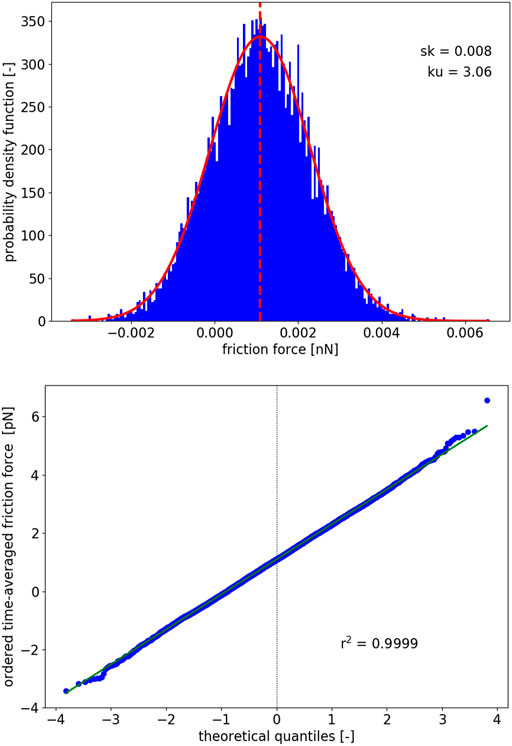
FIGURE 3. In the top panel, the histogram of the time-averaged friction force (blue) for the same sliding experiment repeated 10⁴ times together with the corresponding normal (Gaussian) distribution (solid red line) and the mean (dashed red line). Here the skewness (sk) and kurtosis (ku), i.e., the third and fourth central moments, are measuring the high quality of the normal distribution for the time-averaged friction force. This is additionally also quantified by Pearson’s linear correlation coefficient r² in the bottom panel, where the probability plot of the time-averaged friction force is given.

Furthermore, by inspecting the normal probability plot given in Figure 3B which per definition identifies graphically the departure of random data from normality, i.e., from the Gaussian behavior, it can be observed that the ordered time-averaged friction force shows against the theoretical quantiles q_i (i = 1, …, n − 1) indeed a perfect linear correlation in terms of the Pearson’s coefficient,

$r=\frac{1}{{\sigma }_F{\sigma }_q}\frac{1}{n}\sum _{i=1}^n\left(F_i-⟨\langle F\rangle ⟩\right)\left(q_i-⟨\langle q\rangle ⟩\right),(21)$

where $⟨\langle q\rangle ⟩$ and σ_q denote the mean and standard deviation of q_is. Note that theoretical quantiles are grid-points dividing the range of a probability density function, in our case the Gaussian one, into adjacent intervals of equal probabilities, thus the q_is are values of the inverse cumulative Gaussian density function at i/n. This normal distribution of friction forces persists in all frictional regimes, i.e., in both stick-slip and superlubric regimes, for any material pairing (arbitrary U₀-value), and any strength of the elastic coupling (arbitrary k_c-value) between the AFM-tip and drive as detailed in the Supplementary Material. Even more, also the reaction force aiming the AFM-tip perpendicularly to the friction force to follow the straight sliding path is perfectly normally (Gaussian) distributed, recall Figure 4. Probably, all these statistical features are less surprising for somebody knowing that averages of random numbers of an arbitrary distribution are always normally distributed. Accordingly, as further detailed in the Supplementary Material when applying the 1D PT-model for sake of simplicity, independently of the frictional regime, also the block-averaged time-dependent friction force is normally (Gaussian) distributed. Formally, this is still a direct consequence of the averaging and not necessarily of the fact that the time-dependent friction force is normally distributed too due to the Gaussian-shape of the thermal-noise-induced random force in Eq. 4.

FIGURE 4

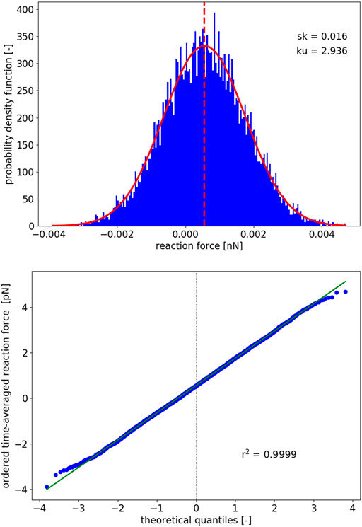
FIGURE 4. As in Figure 3, for the reaction force.

Since our main goal is to numerically study the occurrence of structural superlubricity as function of various parameters, such as temperature and velocity, for example, a 10⁴ times repetition of the sliding for a single parametric configuration is too demanding computationally and therefore one should develop a numerical scheme to achieve accurate approximations of $⟨F⟩$ and σ_F, recall Eq. 18, by performing much fewer repetitions n ≪ 10⁴. In a first attempt, it was taken advantage on the central limit theorem stating that the composite variable $z_n=\sqrt{n}\left({⟨\langle F\rangle ⟩}_n-⟨\langle F\rangle ⟩\right)/{\sigma }_F$, with ${⟨\langle F\rangle ⟩}_n$ as introduced in Eq. 16, tends to be normally distributed with zero mean and unity standard deviation, i.e., $\mathcal{N}\left(z_n|\mathrm{0,1}\right)$ in accordance with Eq. 19, when the number of repetitions n goes to infinity. This in terms of distribution means that the probability $P\left(z_n\le z_{\sup }\right)$ tends to the cumulative Gaussian density function at z_sup, i.e., the supremum of z_n, when n → ∞. Indeed, by setting the accuracy for fulfilling the latter identity, one could have reasonable ${⟨\langle F\rangle ⟩}_n$ and σ_n, recall Eq. 17, in comparison with $⟨\langle F\rangle ⟩$ and σ_F for n in range of thousands as presented in Supplementary Material. Unfortunately, for a large-parametric study of structural superlubricity, thousands of repetitions per configuration are still too high.

In a next attempt, it was iteratively attempted to achieve the convergence of the mean force. 1) In a first step, one increases step-by-step the number of repetitions n until the mean ${⟨\langle F\rangle ⟩}_n$ becomes zero or positive-valued. 2) Then the repetitions are further increased step-by-step until the mean ${⟨\langle F\rangle ⟩}_{n+m}$ will be again zero or positive. 3) If the difference of these means $\left|{⟨\langle F\rangle ⟩}_n-{⟨\langle F\rangle ⟩}_{n+m}\right|$ is below a given positive threshold ${ϵ}_{⟨F⟩}$, then it is assumed that the convergence is achieved, and one considers $\left({⟨\langle F\rangle ⟩}_n+{⟨\langle F\rangle ⟩}_{n+m}\right)/2$ as being the accurate mean. 4) Otherwise, the algorithm is continued from 1) by setting n to n + m. Unfortunately, in this iterative scheme too the number of repetitions n remains to be of order of 10³, see depicted in Supplementary Material.

Finally, it was decided to realize the convergence of the mean friction and/or reaction force by setting the accuracy ϵ_G > 0 with which the normality of forces should be achieved. Namely, increasing either step-by-step or blockwise the number of repetitions, it is continuously verified whether ${⟨\langle F\rangle ⟩}_n\ge 0$ and simultaneously the skewness together with the kurtosis, recall Eq. 20, are accurate enough, i.e.,

$\left|{\mathrm{s}\mathrm{k}}_n\right|\le {ϵ}_G\&\left|{\mathrm{k}\mathrm{u}}_n-3\right|\le {ϵ}_G.(22)$

If these criteria are satisfied, the mean of friction and reaction forces are considered to be converged and the normality of their distributions is additionally quantified by Pearson’s linear correlation coefficient, recall Eq. 21. For the case that one of the criteria in Eq. 22 and/or ${⟨\langle F\rangle ⟩}_n\ge 0$ could not be fulfilled, a predefined maximum number of repetitions n_max, e.g., 10⁴, will be performed by assuming that this n_max is large enough for obtaining good mean values for the forces. What one observes in Figure 5 is that by decreasing ϵ_G for the skewness and kurtosis, the normality of friction force is increasing as quantified by these moments and also by Pearson’s (linear) correlation coefficient. However, after a while a further decease of ϵ_G does not really improve the positive mean ${⟨\langle F\rangle ⟩}_n$ in comparison with ${⟨\langle F\rangle ⟩}_{10^4}$ taken as reference when n = 10⁴. From Figure 6 it becomes evident that a relatively large ϵ_G = 0.2 is recommended for using within the stick-slip regime leading to a couple of tenths of repetitions and hence to a fast convergence of the mean values for forces, whereas a ten times smaller ϵ_G = 0.02 is suitable to achieve highly accurate means of forces with the superlubric regime by performing a couple of hundreds of repetitions.

FIGURE 5

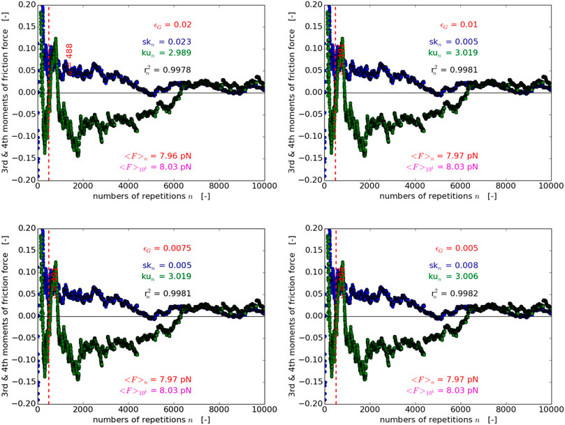
FIGURE 5. Convergence of the friction force skewness (blue) and kurtosis (green) within the 1D PT-model, together with the number n of repetitions needed (red dashed line) to achieve a given accuracy ɛ_G, and to this accuracy corresponding Pearson’s linear correlation coefficient $r_n^2$. In addition, the mean of the friction force ⟨ F ⟩_n is compared with the reference mean ${⟨F⟩}_{10^4}$ obtained by repeating 10⁴ times one and the same numerical AFM-experiment.

FIGURE 6

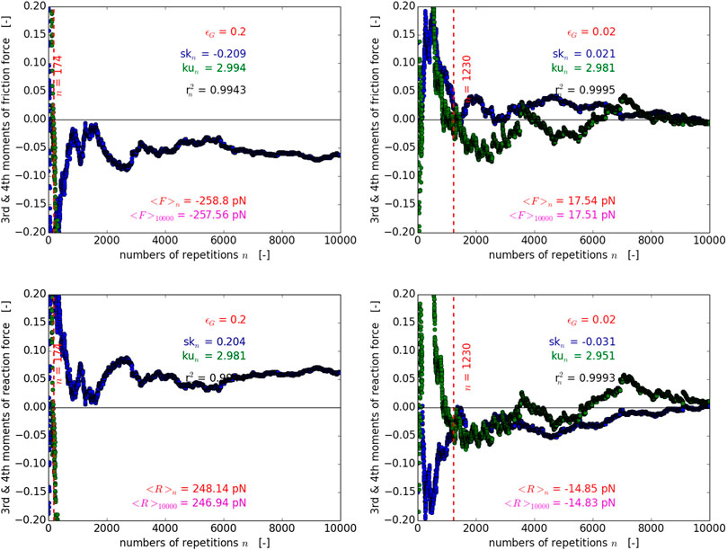
FIGURE 6. As in Figure 5, for the friction (top row) and reaction force (bottom row) within a stick-slip (left panels) and a superlubric frictional regime (right panels) obtained by applying the 2D PT-model.

6 Large-Parametric Studies

Having fixed the convergence criteria with ϵ_G = 0.02, large parametric studies of sliding along (in)commensurate paths were performed first using the 1D PT-model. By varying the system and environment properties, we aim to gain understanding on the dependence of the friction forces and thus the frictional regime on any of these parameters. As illustrated in Figure 7, the temperature values of T = 0 K and T = 300 K were considered when solving the corresponding ODEs and SDEs respectively. In these calculations, the η-dependence of structural superlubricity was studied by keeping all parameters entering Eq. 1 constant, except the corrugation potential amplitude U₀ and the spring constant of the coupling of the AFM-tip to the drive k_c, respectively, which were varied independently. A different behaviour is observed in the case of each variation.

FIGURE 7

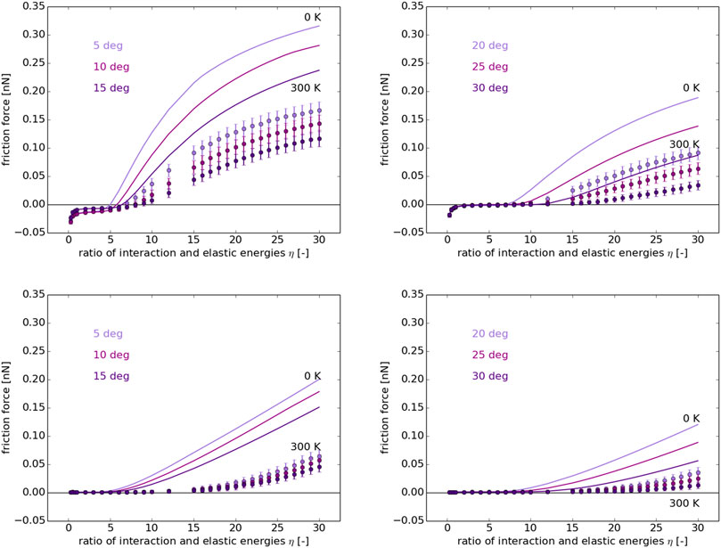
FIGURE 7. η-dependence of structural superlubricity as predicted by the 1D PT-model at 0 K (solid line) and at RT of 300 K (full circles) along various incommensurate sliding paths Φ = 5, 10, 15, 20, 25 and 30 deg (depicted in violet as specified in the legend), recall Figures 1, 2, when either U₀(top row) or k_c(bottom row) is kept constant in Eq. 14.

When U₀ is kept constant, one can observe a short region of very low friction forces, followed by a quick increase with a diminishing slope as the ratio η increases. The introduction of thermal noise at non-zero temperatures leads to the reduction of the friction forces in the stick-slip regime, however, the region of the superlubric regime is not significantly affected. At very low η values, which correspond to very high spring constants k_c, negative friction force values of low magnitude are observed. This can be due to the non-convergence of the average force, as it was already observed that a larger number of statistically independent realisations is typically required in the superlubric regime. On the other hand, it could pinpoint to an incompatibility of the very high elastic coupling energy for the given interaction energy of the AFM-tip with the surface, where the assumptions of the PT-model may not be valid.

In the opposite case where the spring constant k_c is kept fixed and the interaction potential is varied, only positive friction forces are observed. The superlubric regime holds for larger values of η, while the increase of forces is less abrupt and shows a linear trend. Here, the introduction of thermal noise also leads to a reduction of the friction forces, however, it also leads to a significant expansion of the range of η values which lead to a superlubric regime. It becomes clear, therefore, from the analysis of Figure 7 that the value of η uniquely determines the type of frictional regime, either stick-slip or superlubric between the AFM-tip and any semi-infinite crystalline substrate.

Note that all these numerical studies evidence significantly larger intervals for η where the superlubric frictional regime could occur than that of η < 1 assumed in the literature for both U₀ and k_c kept constant, recall for example Ref. (Socoliuc et al., 2004). This means that by varying the material and system properties, the occurrence of superlubricity could be further tuned and even extended on (in)commensurate sliding paths. Furthermore, it seems also that the superlubricity for η < 1, recall Figure 7, it is more pronounced than over its extension for 1 ≤ η < 20, probably because the former is energetically and the latter symmetrically more favorable. Even small negative values for friction force are obtained when η < 1 and U₀ is varied, which shows that probably a sliding distance of only 3.5 nm which was considered here, is not enough to get in average the drive in front of the AFM-tip.

All the same holds for the friction forces calculated using the 2D PT-model, cf. Figure 7 with the left panels of Figure 8. What concerns the η-dependence of the reaction force, this differs not too much from that of the friction force, as one observes on the right column of Figure 8, and shows that keeping the sliding on an incommensurate path needs in magnitude higher reaction forces, when η increases. Interestingly, the incommensurate paths are not equivalent, since the η-dependence of the friction and reaction forces is Φ-dependent too. Furthermore, both forces, i.e., the frictional in both 1D and 2D PT-models, and the reaction force within the 2D PT-model, feature a strong temperature dependence for a given sliding velocity.

FIGURE 8

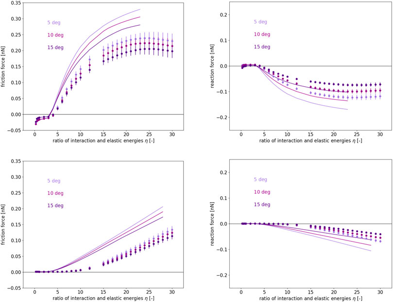
FIGURE 8. As in Figure 7, for three two-dimensional incommensurate sliding paths Φ = 5, 10 and 15 deg, when using the 2D PT-model.

Apart from identifying the frictional regime according to the material and system properties, the 1D and 2D PT-models also enable us to study the temperature and velocity dependence of friction and reaction forces in both stick-slip and superlubric frictional regimes. In Figures 9, 10 only the calculated friction force for a large range of temperature and sliding velocity values is given, because in magnitude much smaller reaction force behaves pretty similarly. It can be readily observed that the increase of temperature leads to a monotonic decrease of friction forces within both frictional regimes, as the increasing thermal motion aids the AFM-tip to overcome the interaction energy barriers and slide with a lower mechanical energy. On the other hand, the increase of sliding velocity results in increased friction forces strongly depending on the frictional regime, probably due to different impact of the damping. A linear dependence of the friction and reaction force (although the latter is not shown explicitly here) on the logarithm of the sliding velocity can be observed within the stick-slip regime,

$\left(a_1{k}_{\text{B}}T+a_0\right)\ln \frac{v_s}{v_s^{(\mathrm{r}\mathrm{e}\mathrm{f})}},(23)$

of which slope a₁k_BT + a₀ is linearly depending on the absolute temperature T. In this Eq. 23k_B stands for the Boltzmann constant and $v_s^{(\mathrm{r}\mathrm{e}\mathrm{f})}$ denotes the selected reference sliding velocity, here and in the following, the minimum of all considered sliding velocities. Within the superlubric frictional regime, a similar functional dependence as in Eq. 23 holds only when U₀ is varied. When k_c is varied, then the quadratic form

$\left[a_2{(k_{\text{B}}T)}^2+a_1{k}_{\text{B}}T+a_0\right]{\left[\ln \frac{v_s}{v_s^{(\mathrm{r}\mathrm{e}\mathrm{f})}}\right]}^2,(24)$

provides the temperature and sliding velocity dependence of the friction and reaction forces. For the values of the polynomial coefficients a_p (p = 0, 1, 2) and further computational details, see the Supplementary Material. All these are suggesting at least a power-law dependence of friction reaction force on the sliding velocity with a temperature-dependent exponent.

FIGURE 9

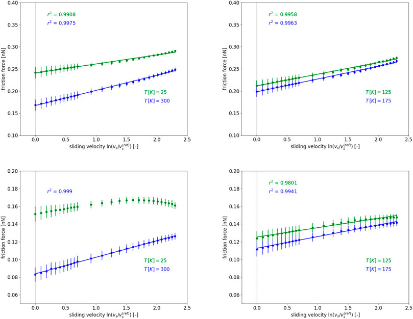
FIGURE 9. Temperature and sliding velocity dependence of the friction force as predicted by the 2D PT-model within the stick-slip regime along the incommensurate path for Φ = 15 deg, when either U₀(top row) or k_c(bottom row) is kept constant in Eq. 14.

FIGURE 10

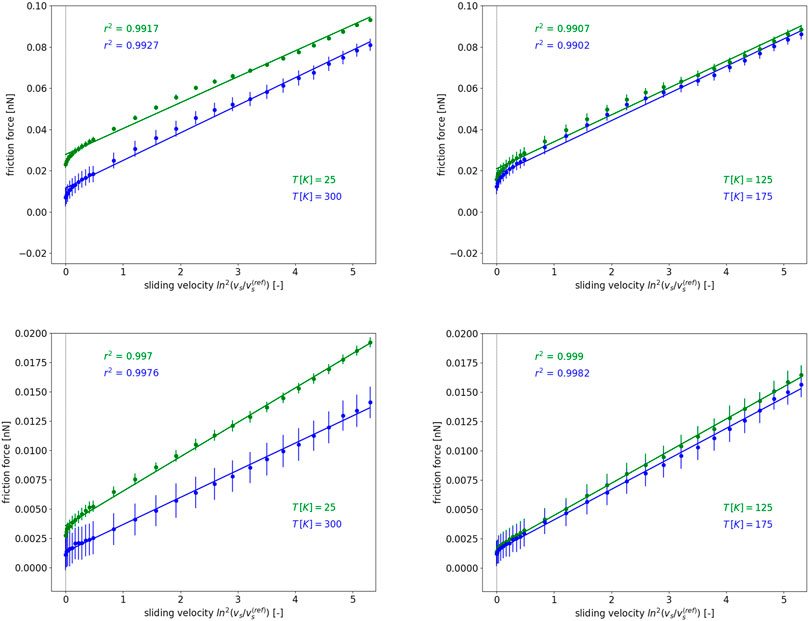
FIGURE 10. As in Figure 9, but within the superlubric frictional regime.

7 Summary and Conclusions

In summary, the PT-model was considered in one and two dimensions for the numerical description of an AFM-tip sliding over a periodic and atomically flat surface. A system of SDEs was considered and implemented for the inclusion of the effects of temperature on the motion of the tip. The conditions for the derivation of statistically accurate friction and reaction forces in a numerically efficient way were defined. The proposed statistically proper scheme can be applied for sliding on both commensurate and incommensurate paths, while it allows the study of the impact of both system and environmental conditions on the resulting friction forces.

By the numerical study of the AFM-tip sliding using the PT-models, it was concluded that the ratio between the mean interaction energy of the AFM-tip with the surface and the elastic energy of spring coupling the AFM-tip to the drive, can uniquely determine the type of frictional regime, either stick-slip or superlubric between the AFM-tip and any semi-infinite crystalline substrate. In addition, the friction force in both regimes is predicted to be a function of temperature and sliding velocity.

All these findings can support the design of appropriate experimental studies for the realization of structural superlubricity, while they can also shed light into the design of novel systems showing ultra-low friction which can be beneficial in several engineering applications.

Data Availability Statement

The original contributions presented in the study are included in the article/Supplementary Material, further inquiries can be directed to the corresponding author.

Author Contributions

MS: made the calculations and representation of data KG: wrote the manuscript and interpretation of data CG: interpretation of data and discussions AV: developed the theory, made the programming, wrote the manuscript.

Funding

This work was funded by the Austrian COMET-Project INTRIBOLOGY (FFG-No. 872176) and carried out at the “Excellence Centre of Tribology” (AC2T research GmbH). MS, KG, and AV have received funding also from the European Union’s Horizon 2020 research and innovation prgramme under grant agreement No. 814494, project i-TRIBOMAT.

Conflict of Interest

Authors MS and AV were employed by company AC2T Research GmbH, whereas author KG was employed by Toyota Motor Europe NV/SA.

The remaining author declares that the research was conducted in the absence of any commercial or financial relationships that could be construed as a potential conflict of interest.

Publisher’s Note

All claims expressed in this article are solely those of the authors and do not necessarily represent those of their affiliated organizations, or those of the publisher, the editors and the reviewers. Any product that may be evaluated in this article, or claim that may be made by its manufacturer, is not guaranteed or endorsed by the publisher.

Acknowledgments

The authors acknowledge TU Wien Bibliothek too for financial support through its Open Access Funding Program.

Supplementary Material

The Supplementary Material for this article can be found online at: https://www.frontiersin.org/articles/10.3389/fmech.2021.742684/full#supplementary-material

References

Butcher, J. C., and Wanner, G. (1996). Runge-kutta Methods: Some Historical Notes. Appl. Numer. Maths. 22, 113–151. doi:10.1016/s0168-9274(96)00048-7

CrossRef Full Text | Google Scholar

Dong, Y., Vadakkepatt, A., and Martini, A. (2011). Analytical Models for Atomic Friction. Tribol. Lett. 44, 367–386. doi:10.1007/s11249-011-9850-2

CrossRef Full Text | Google Scholar

A. Erdemir, and J.-M. Martin (Editors) (2007). Superlubricity (Amsterdam: Elsevier).

Google Scholar

A. Erdemir, J.-M. Martin, and J. Luo (Editors) (2021). Superlubricity (Amsterdam: Elsevier).

Google Scholar

Filippov, A. E., Vanossi, A., and Urbakh, M. (2010). Origin of Friction Anisotropy on a Quasicrystal Surface. Phys. Rev. Lett. 104, 074302. doi:10.1103/PhysRevLett.104.074302

PubMed Abstract | CrossRef Full Text | Google Scholar

Hirano, M., and Shinjo, K. (1990). Atomistic Locking and Friction. Phys. Rev. B 41, 11837–11851. doi:10.1103/physrevb.41.11837

PubMed Abstract | CrossRef Full Text | Google Scholar

Hirano, M., Shinjo, K., Kaneko, R., and Murata, Y. (1991). Anisotropy of Frictional Forces in Muscovite Mica. Phys. Rev. Lett. 67, 2642–2645. doi:10.1103/physrevlett.67.2642

PubMed Abstract | CrossRef Full Text | Google Scholar

Kalogiratou, Z., Monovasilis, T., Psihoyios, G., and Simos, T. E. (2014). Runge-kutta Type Methods with Special Properties for the Numerical Integration of Ordinary Differential Equations. Phys. Rep. 536, 75–146. doi:10.1016/j.physrep.2013.11.003

CrossRef Full Text | Google Scholar

Kasdin, N. J. (1995). Runge-kutta Algorithm for the Numerical Integration of Stochastic Differential Equations. J. Guidance, Control Dyn. 18 (1), 114–120. doi:10.2514/3.56665

CrossRef Full Text | Google Scholar

Kobayashi, K., Liang, Y., Amano, K.-i., Murata, S., Matsuoka, T., Takahashi, S., et al. (2016). Molecular Dynamics Simulation of Atomic Force Microscopy at the Water-Muscovite Interface: Hydration Layer Structure and Force Analysis. Langmuir 32 (15), 3608–3616. doi:10.1021/acs.langmuir.5b04277

PubMed Abstract | CrossRef Full Text | Google Scholar

Krylov, S. Y., Jinesh, K. B., Valk, H., Dienwiebel, M., and Frenken, J. W. (2005). Thermally Induced Suppression of Friction at the Atomic Scale. Phys. Rev. E Stat. Nonlin Soft Matter Phys. 71, 065101. doi:10.1103/PhysRevE.71.065101

PubMed Abstract | CrossRef Full Text | Google Scholar

Kutta, W. (1901). Beitrag zur näherungsweisen Integration totaler Differentialgleichungen. Z. Math. Phys. 46, 435.

Google Scholar

Martin, J. M., and Erdemir, A. (2018). Superlubricity: Friction's Vanishing Act. Phys. Today 71 (4), 40–46. doi:10.1063/pt.3.3897

CrossRef Full Text | Google Scholar

Pawlak, R., Ouyang, W., Filippov, A. E., Kalikhman-Razvozov, L., Kawai, S., Glatzel, T., et al. (2016). Single-Molecule Tribology: Force Microscopy Manipulation of a Porphyrin Derivative on a Copper Surface. ACS Nano 10 (1), 713–722. doi:10.1021/acsnano.5b05761

PubMed Abstract | CrossRef Full Text | Google Scholar

Peng, Y., Zeng, X., Yu, K., and Lang, H. (2020). Deformation Induced Atomic-Scale Frictional Characteristics of Atomically Thin Two-Dimensional Materials. Carbon 163, 186–196. doi:10.1016/j.carbon.2020.03.024

CrossRef Full Text | Google Scholar

Popov, V. L., and Gray, J. A. T. (2012). Prandtl-Tomlinson Model: History and Applications in Friction, Plasticity, and Nanotechnologies. Z. Angew. Math. Mech. 92 (9), 683–708. doi:10.1002/zamm.201200097

CrossRef Full Text | Google Scholar

Prandtl, L. (1928). Ein Gedankenmodell zur kinetischen Theorie der festen Körper. Z. Angew. Math. Mech. 8, 85–106. doi:10.1002/zamm.19280080202

CrossRef Full Text | Google Scholar

Press, W. H., Teukolsky, S. A., Vetterling, W. T., and Flannery, B. P. (2007). Numerical Recipes – the Art of Scientific Computing. Cambridge: University Press.

Google Scholar

Runge, C. (1895). Über die numerische Auflösung von Differentialgleichungen. Math. Ann. 46, 167–178. doi:10.1007/bf01446807

CrossRef Full Text | Google Scholar

Schwarz, U. D., and Hölscher, H. (2016). Exploring and Explaining Friction with the Prandtl-Tomlinson Model. ACS Nano 10 (1), 38–41. doi:10.1021/acsnano.5b08251

PubMed Abstract | CrossRef Full Text | Google Scholar

Socoliuc, A., Bennewitz, R., Gnecco, E., and Meyer, E. (2004). Transition from Stick-Slip to Continuous Sliding in Atomic Friction: Entering a New Regime of Ultralow Friction. Phys. Rev. Lett. 92, 134301. doi:10.1103/physrevlett.92.134301

PubMed Abstract | CrossRef Full Text | Google Scholar

Tomlinson, G. A. (1929). CVI.A Molecular Theory of Friction. Lond. Edinb. Dublin Philos. Mag. J. Sci. 7, 905–939. doi:10.1080/14786440608564819

CrossRef Full Text | Google Scholar

Wolloch, M., Feldbauer, G., Mohn, P., Redinger, J., and Vernes, A. (2015). Ab Initiocalculation of the Real Contact Area on the Atomic Scale. Phys. Rev. B 91, 195436. doi:10.1103/physrevb.91.195436

CrossRef Full Text | Google Scholar