Sensor System and Observer Algorithm Co-Design For Modern Internal Combustion Engine Air Management Based on H2 Optimization

This paper outlines a novel sensor selection and observer design algorithm for linear time-invariant systems with both process and measurement noise based on H₂ optimization to optimize the tradeoff between the observer error and the number of required sensors. The optimization problem is relaxed to a sequence of convex optimization problems that minimize the cost function consisting of the H₂ norm of the observer error and the weighted l₁ norm of the observer gain. An LMI formulation allows for efficient solution via semi-definite programing. The approach is applied here, for the first time, to a turbo-charged spark-ignited engine using exhaust gas circulation to determine the optimal sensor sets for real-time intake manifold burnt gas mass fraction estimation. Simulation with the candidate estimator embedded in a high fidelity engine GT-Power model demonstrates that the optimal sensor sets selected using this algorithm have the best H₂ estimation performance. Sensor redundancy is also analyzed based on the algorithm results. This algorithm is applicable for any type of modern internal combustion engines to reduce system design time and experimental efforts typically required for selecting optimal sensor sets.

1 Introduction

The control of fuel and air in spark-ignited engines has increasingly become a challenge with the incorporation of turbo-charging, exhaust gas recirculation (EGR), valvetrain flexibility, and more stringent emission regulations. To enable effective stoichiometric air-to-fuel ratio control, the engine flow and composition must be accurately and robustly measured or estimated. The only viable option is to use algorithms to estimate the engine mass flow and composition. Five difficulties have to be taken into consideration for the engine air handling sensor and observer (i.e. estimator) design problem: 1) nonlinear system dynamics; 2) measurement uncertainties, including sensor delays and noise; 3) multivariate interactions; 4) engine variability for different operation conditions and 5) the trade-off between estimation accuracy and sensor costs.

Previous studies in the field of engine air handling system management have focused on the observer design based on pre-selected sensor sets (Wang, 2008; Simon and Garg, 2010; Chen and Wang, 2012; Rengarajan et al., 2018). However, considering the increasing complexity of today’s engine systems and sensor characteristics, the choice of optimal air handling sensor set is not obvious; and it can be time-consuming and error prone if ‘guess and check’ experimental or simulation approaches are used. With the increasing variety of available sensors, the possible combinations of sensors will grow quickly. Brute-force experimentation with different sensors is very expensive and time-consuming, and may need to be redone even when there are minor changes to the engine system or control strategies. In order to effectively solve the problem, an algorithm for optimal sensor selection and observer design for the engine air handling system is outlined and demonstrated in this paper.

As described in more detail in the following paragraphs, several mathematical methods have been developed to solve the sensor selection problem, including greedy algorithms and convex optimization. Greedy algorithms aim to find a global optimum by making the locally optimal choice at each stage. The solution computed by the greedy algorithm is not always globally optimal. Convex optimization problems have the property that any found local optimal will also be global. While most formulations are nonconvex, sometimes it is possible to convexify them with minimum or no impact on the solution to take advantage of the solution properties as well as of available solvers (Joshi and Boyd, 2008; Tropp, 2006; Luo et al., 2010).

Sensor selection methods have been applied to various areas. In Kalandros and Pao (1998), the authors proposed three sensor selection algorithms for signal target tracking problems based on different resource and performance metrics. In another paper Kalandros et al. (1999), the authors explored the use of randomization and a super-heuristic in multiple targets tracking problem to improve any given sensor set solution via random perturbation. That approach is more suitable for systems with little structure and for which the cost of solution evaluation is not high. In Hashemi et al. (2018), the authors studied a randomized greedy algorithm for near-optimal sensor scheduling in large-scale sensor networks. In Rao et al. (2015), a greedy algorithm based on two submodular cost functions, the weighted frame potential and the weighted log-det, was developed for the sensor selection problem in non-linear measurement models with additive normally distributed noise. Several sensor selection algorithms based on convex optimization or relaxation have also been applied to flexible structures. In Fardad et al. (2011), Münz et al. (2014), Zare and Jovanović (2018), and Dhingra et al. (2014), the weighed l₁ norm (without considering measurement noise) or l₂ norm of the observer gain was used to represent the sensor number, and minimized along with the H₂ norm of the estimation error. The optimization problem was solved via SDP (Fardad et al., 2011; Münz et al., 2014), alternating direction method of multipliers (ADMM) (Zare and Jovanović, 2018) and proximal methods (Dhingra et al., 2014). In Chepuri and Leus (2014), several functions of the Cramer–Rao bound (CRB) were used as a performance measure and the sensor selection problem was formulated to minimize the CRB functions and a sparse selection vector. In Joshi and Boyd (2008), the authors computed the optimal sensor set among candidate linear measurements corrupted with normally distributed noises. The maximum-likelihood estimation errors were used as the performance evaluations.

In the application of engine sensor selection, methods include experimentation-based sensor selection and algorithm-based sensor selection. In Pekař et al. (2012), the best sensor configuration for a heavy-duty engine was found based on experimental results by testing each sensor design. In Mushini and Simon (2005), the authors implemented a sensor selection algorithm for aircraft gas turbine engine healthy parameter estimation by minimizing the cost function of the estimation error and financial cost via a greedy algorithm. In Suard et al. (2008), the authors determined the best sensor configurations among three candidate sensor configurations for air-fuel-ratio control in a spark ignited engine. Different controllers were designed for candidate sensor configurations. An objective function incorporating the overall system cost and controller performance as the optimization target was used, with solution via a genetic algorithm. In Palmer et al. (2018), the authors proposed a methodology for fault diagnosis sensor selection based on D_s optimal FDI test design that maximized the sensitivity of outputs to anticipated faults and applied it in a diesel engine air handling system. The problem was solved using a heuristic method.

In the work described here, a simultaneous, coupled sensor selection and observer design method for the air handling system of the turbo-charged SI engine with EGR is proposed. In a manner similar to the approach taken in (Fardad et al., 2011; Münz et al., 2014), the strategy uses H₂ optimization and accounts for both process and measurement noise. The goal of this algorithm is to definitively, and accurately, determine the tradeoff between the necessary sensor number and the accuracy of intake manifold oxygen fraction estimation. The implemented cost function consists of the H₂ norm of the observer error and the weighted l₁ norm of the observer gain. The problem, once formulated, can be solved efficiently via semi-definite programming (SDP). After selecting the optimal sensor set, the algorithm computes the corresponding Kalman-filter gain based on the selected sensor set. A method to estimate the modeling errors based on the comparison of reference data and modeling data is also proposed in this paper, enabling the application of the sensor selection framework to physical systems.

The rest of the paper is organized as follows: The statement of the sensor selection problem and its convex formulation; The application of the algorithm on a spark-ignited (SI) engine for intake manifold burnt gas mass fraction estimation for medium/high-speed operating conditions; Conclusions; Future work.

2 Sensor Selection Algorithm Based on H₂ Optimization

Considering the following linear continuous state space model:

$\begin{array}{l}\dot{x}=Ax+Bu+B_d{u}_d+B_{w}w\\ y=Cx+Du+D_d{u}_d+Hv\end{array}(1)$

with the state variables $x\in R^m$, measured outputs $y\in R^n$, control inputs $u\in R^p$, disturbance inputs $u_d\in R^s$, unknown disturbance related to model uncertainty $w\in R^m$, and sensor noise $v\in R^n$. Both w and v are modeled as white noise. $B_w\in R^{m\times m}$ and $H\in R^{n\times n}$ are diagonal magnitude matrices.

A Luenberger observer then takes the form:

$\begin{array}{c}\dot{\widehat{x}}=A\widehat{x}+Bu+B_d{u}_d+L\left(y-\widehat{y}\right)\\ \widehat{y}=C\widehat{x}+Du+D_d{u}_d\\ z=We=W\left(x-\widehat{x}\right)\end{array}(2)$

where $L\in R^{m\times n}$ is the observer gain, $z\in R^q$ is the weighted error and $W\in R^{q\times m}$ is the weighting matrix to address some errors from all state errors.

By introducing the following two matrices:

$\begin{array}{l}{\tilde{B}}_w^{m\times \left(m+n\right)}=\left[\begin{array}{cc}{B}_w^{m\times m}& 0^{m\times n}\end{array}\right]\\ {\tilde{H}}^{n\times \left(m+n\right)}=\left[\begin{array}{cc}{0}^{n\times m}& H^{n\times n}\end{array}\right]\end{array}(3)$

the weighted error z can be formulated as:

$z=W{\left(sI-A+LC\right)}^{-1}\left({\tilde{B}}_w-L\tilde{H}\right)\left[\frac{w}{v}\right]=G\left[\frac{w}{v}\right](4)$

where the error system G is the transfer function matrix between $\left[\frac{w}{v}\right]$ and z.

2.1 Cost Function

For MIMO systems, the H₂ norm is the impulse-to-energy gain or steady-state variance of outputs in response to white noise (Arzelier, 2008). Therefore, by minimizing the H₂ norm of the error system (4), the expected root-mean-square error (RMSE) of the observer in response to white noise input excitation is minimized. The H₂ norm of the error system G in Eq. 4 is expressed as:

${\Vert G\Vert }_2=\sqrt{\mathcal{E}\left\{\underset{t\to \infty }{\lim }\frac{1}{t}{\displaystyle {\int }_0^t{z}^T\left(t\right)z\left(t\right)}\text{d}t\right\}}(5)$

where $\mathcal{E}$ is the expectation operator.

Considering the observer gain matrix L, the corresponding jth sensor measurement does not contribute to the state estimation results if every element in the jth column of L is zero. In this case, the absolute sum of the elements in jth column of L is also zero. The number of sensors can be reduced by minimizing the non-zero columns in L, which is the $l_0$ norm of the row vector $p\in R^{1\times n}$ of absolute column sum of L, i.e., ${\Vert p\Vert }_0={\displaystyle \sum _{j=1}^n{\left|\left|{\displaystyle \sum _{i=1}^m\left|L_{ij}\right|}\right|\right|}_0}$.

In order to optimize the tradeoff between the observer estimation error and the number of required sensors, a cost function is defined as following:

$J=\left(1-\alpha \right){\Vert G\Vert }_2^2+\alpha {\displaystyle \sum _{j=1}^n{\left|\left|{\displaystyle \sum _{i=1}^m\left|L_{ij}\right|}\right|\right|}_0}(6)$

where ${\Vert G\Vert }_2$ denotes the H₂ norm of the error system or the expected root-mean square weighted error, and α is the weighting factor between 0 and 1, balancing the effect of observer error and sensor number.

2.2 H₂ Norm of the Observer Error

From Peet (2016), for a LTI system with a transfer function $G\left(s\right)=C{\left(sI-A\right)}^{-1}B$, the following statements are equivalent:

(1) A is Hurwitz and ${\Vert G\Vert }_2^2$ (the power of H₂ norm of the impulse response) $<{\gamma }^2$.

(2) There exists a positive definite matrix P (i.e., $P=P^T\succ 0$) such that

$\begin{array}{l}{A}^{T}P+PA+C^{T}C\prec 0\\ trace\left(B^{T}PB\right)<{\gamma }^2\end{array}(7)$

where the symbol $\prec$ in the first inequality of Eq. 7 denotes the negative definiteness of a matrix.

By applying Eq. 7 to system (4), the optimization problem for the first target ${\Vert G\Vert }_2^2$ in Eq. 6 can be formulated as following:

$\begin{array}{l}\underset{L,P}{\min }trace\left({\left({\tilde{B}}_w-L\tilde{H}\right)}^{T}P\left({\tilde{B}}_w-L\tilde{H}\right)\right)\\ s.t{\left(A-LC\right)}^{T}P+P\left(A-LC\right)+W^{T}W\prec 0\\ P=P^T\succ 0\end{array}(8)$

The optimization target and the first constraint in (8) are bilinear matrix inequalities (BMI) and is thus not a convex optimization problem. Therefore, they need to be converted to linear matrix inequalities (LMI). A matrix $S=PL$ (thus $L=P^{-1}S$) is defined and the first constraint in Eq. 8 can be written as the following LMI:

$A^{T}P+PA-C^T{S}^T-SC+W^{T}W\prec 0(9)$

Via the Schur complement condition for positive semi-definiteness (Chong and Zak, 2013), the following two statements are equivalent:

(1) Symmetric matrix $\left[\begin{array}{cc}{\Delta }_1& {\Delta }_2\\ {\Delta }_2^T& {\Delta }_3\end{array}\right]\underset{¯}{\succcurlyeq }0$

(2) ${\Delta }_3={\Delta }_3^T\succ 0$ and ${\Delta }_1-{\Delta }_2{\Delta }_3^{-1}{\Delta }_2^T\underset{¯}{\succcurlyeq }0$

To apply the Schur complement condition to the optimization target Eq. 8, we introduce a positive semi-definite matrix T, i.e., $T=T^T\underset{¯}{\succ }0$. By substituting ${\text{Δ}}_1=T$, ${\text{Δ}}_2={\left(P{\tilde{B}}_w-S\tilde{H}\right)}^T$ and ${\text{Δ}}_3=P$, the following statement holds:

$\left[\begin{array}{cc}T& {\left(P{\tilde{B}}_w-S\tilde{H}\right)}^T\\ P{\tilde{B}}_w-S\tilde{H}& P\end{array}\right]\underset{¯}{\succcurlyeq }0,P=P^T\succ 0(10)$

iff

$T-{\left(P{\tilde{B}}_w-S\tilde{H}\right)}^T{P}^{-1}\left(P{\tilde{B}}_w-S\tilde{H}\right)\underset{¯}{\succcurlyeq }0,P=P^T\succ 0(11)$

The inequality in Eq. 11 can be rewritten as:

$\begin{array}{l}T-{\left(P{\tilde{B}}_w-S\tilde{H}\right)}^T{P}^{-1}\left(P{\tilde{B}}_w-S\tilde{H}\right)\\ =T-{\left(P{\tilde{B}}_w-S\tilde{H}\right)}^T{P}^{-1}P{P}^{-1}\left(P{\tilde{B}}_w-S\tilde{H}\right)\\ =T-{\left(P^{-1}P{\tilde{B}}_w-P^{-1}S\tilde{H}\right)}^{T}P\left(P^{-1}P{\tilde{B}}_w-P^{-1}S\tilde{H}\right)\\ =T-{\left({\tilde{B}}_w-L\tilde{H}\right)}^{T}P\left({\tilde{B}}_w-L\tilde{H}\right)\end{array}(12)$

Therefore, the following statement holds if condition (10) meets:

$trace\left(T\right)\ge trace\left({\left({\tilde{B}}_w-L\tilde{H}\right)}^{T}P\left({\tilde{B}}_w-L\tilde{H}\right)\right)(13)$

Therefore, the optimization problem in (8) can be rewritten as:

$\begin{array}{l}\underset{L,P,T}{\min }trace\left(T\right)\\ s.t.A^{T}P+PA-C^T{S}^T-SC+W^{T}W\prec 0\\ \left[\begin{array}{cc}T& {\left(P{\tilde{B}}_w-S\tilde{H}\right)}^T\\ P{\tilde{B}}_w-S\tilde{H}& P\end{array}\right]\underset{¯}{\succcurlyeq }0\\ P=P^T\succ 0\\ T=T^T\underset{¯}{\succcurlyeq }0\end{array}(14)$

where the root of $trace\left(T\right)$ is the upper bound of the expected weighted root-mean-square error z. In Eq. 8, the optimization target is the H₂ norm of the error system. In Eq. 14, the optimization target is relaxed to the upper bound of the H₂ norm. Here the direct optimization target is $trace\left(T\right)$.

2.3 Weighted l₁ Norm of the Observer Gain Matrix

The second optimization target ${\displaystyle {\sum }_{j=1}^n{\displaystyle {\Vert \sum }_{i=1}^m{|L_{ij}\Vert |}_0}}$ in Eq. 6 is non-convex due to the existing of l₀ norm. For such l₀ norm optimization problem, it is generally impossible to solve as the solution usually requires an intractable combinatorial search (Candes et al., 2008). As proposed in Candes et al. (2008), the l₀ norm term ${\displaystyle {\Vert \sum }_{i=1}^m{|L_{ij}\Vert |}_0}$ can be relaxed to a convex target by using the weighted l₁ norm, ${\mu }_j^{\left(k\right)}{\displaystyle {\sum }_{i=1}^m\left|L_{ij}\right|}$, where ${\mu }_j^{\left(k\right)}$ is the weight of column j at iteration count k.

2.4 Optimization Problem

Using the lemma which is used and proved in Polyak et al. (2013): given a matrix $L\in R^{m\times n}$, the following statements are equivalent:

(1) The jth column of L is zero.

(2) The jth column of $S=PL$ is zero for any $P\succ 0$.

Combine the above lemma with (14) and weighted $l_1$ norm, the optimization problem is formulated as following:

$\begin{array}{l}\underset{S,P,T}{\min }J=\left(1-\alpha \right)trace\left(T\right)+\alpha {\displaystyle \sum _{j=1}^n{\mu }_j^{\left(k\right)}}\stackrel{m}{{\displaystyle \sum }_{i=1}}\left|S_{ij}\right|\\ s.t.A^{T}P+PA-C^T{S}^T-SC+W^{T}W\prec 0\\ \left[\begin{array}{cc}T& {\left(P{\tilde{B}}_w-S\tilde{H}\right)}^T\\ P{\tilde{B}}_w-S\tilde{H}& P\end{array}\right]\underset{¯}{\succcurlyeq }0\\ P=P^T\succ 0\\ T=T^T\underset{¯}{\succcurlyeq }0\end{array}(15)$

The optimization problem (15) can be solved by the CVX toolbox (Grant and Boyd, 2015) iteratively. At each iteration, the algorithm updates the weight factor ${\mu }_j^{\left(k\right)}=\frac{1}{\mathit{ϵ}+{\displaystyle {\sum }_{i=1}^m\left|S_{ij}\right|}}$. When ${\mu }_j^{\left(k\right)}$ converges for all sensor j, i.e., $\left|{\mu }_j^{\left(k+1\right)}-{\mu }_j^{\left(k\right)}\right|<\mathit{ϵ}$ where ϵ is a sufficiently small positive number, the iteration can be stopped.

Ideally, the jth sensor signal is not utilized for the state estimation and should be removed if the jth column of the observer gain matrix L is zero (Münz et al., 2014). Similarly, for a properly scaled system, the signal from sensor(s) j with small ${\displaystyle {\sum }_{i=1}^m\left|L_{ij}\right|}$ will have very little impact on the estimation results and thus can be removed. However, it is hard to quantify the threshold of ‘small’ observer gain and decide the number of sensors that need to be removed. Instead of directly comparing the observer gain of the sensors, the value of ${\displaystyle {\sum }_{j=1}^n{\mu }_j^{\left(k\right)}}{\displaystyle {\sum }_{i=1}^m\left|S_{ij}\right|}$, representing the relaxed non-zero column number in the observer, is checked for every optimization result and used to decide the number of necessary sensors. ${\displaystyle {\sum }_{j=1}^n{\mu }_j^{\left(k\right)}}{\displaystyle {\sum }_{i=1}^m\left|S_{ij}\right|}$ is rounded to its nearest integer q, which is used as the number of selected sensors. For instance, if q is 3 for an optimization result, then the sensor(s) with the first three largest ${\displaystyle {\sum }_{i=1}^m\left|L_{ij}\right|}$ are the selected optimal sensors.

After computing the optimal sensor set, set α to 0 and remove the rows in C corresponding to unneeded sensors. Substitute $\alpha =0$ and the modified C into the optimization algorithm (15) again to calculate the observer gain matrix $L=P^{-1}S$ based only on the selected optimal sensor combination.

3 Algorithm Application on a Turbo-Charged SI Engine Model for Air Handling System Sensor Designs

In this section, the proposed sensor selection algorithm is applied to a turbo-charged SI engine utilizing EGR. The goal of the sensor design is to choose the optimal sensor combination for accurately estimating the intake manifold gas composition. More specifically, the desired outcome is to quickly be able to determine the tradeoff between estimated intake manifold gas composition estimation error and the number of sensors.

The engine architecture is shown in Figure 1. For illustrative purposes, four available sensors are considered as candidates as shown in Table 1. A mass air flow sensor for inlet air (MAFa) can be placed upstream of the air and low pressure (LP) EGR confluence point, to measure the inlet air. A mass air flow sensor for high pressure flow (MAFh) can be placed downstream of the charge air cooler (CAC) to measure the cooled compressor mass flow rate. An EGR delta pressure sensor (EGR DP) can be located in the LP EGR valve to measure the LP EGR mass flow rate. Another option is a mass air flow sensor (MAF) put downstream of the air and LP EGR confluence point, but before the compressor, to measure total compressor inlet mass flow rate.

FIGURE 1

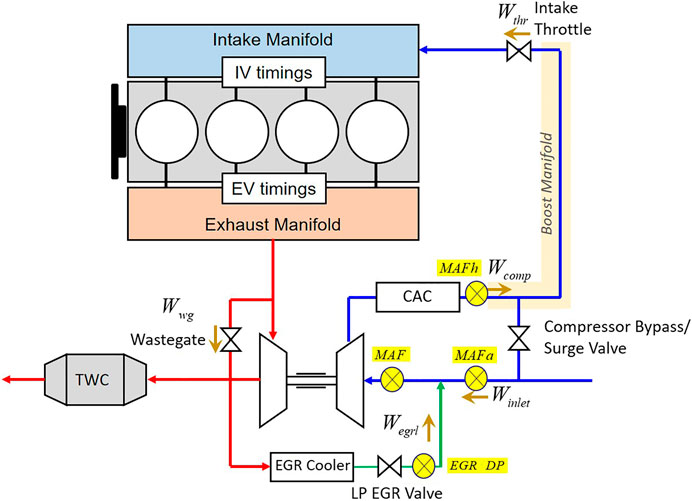
FIGURE 1. Engine architecture and candidate sensor placements.

TABLE 1

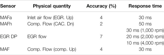
TABLE 1. Available sensors.

3.1 Control-Oriented State-Space Engine Model

The model is a mean-value engine model based on Eriksson and Nielsen (2014), Kocher et al. (2012), Van Alstine et al. (2013), Stricker et al. (2014).

The model has 8 inputs, 1 disturbance input and 20 states as shown in Table 2–4, respectively. The nonlinear dynamic model equations can be written as follows and the detailed governing equations are listed in the Supplemental Material

$\dot{x}=f\left(x,u,u_d\right)(16)$

TABLE 2

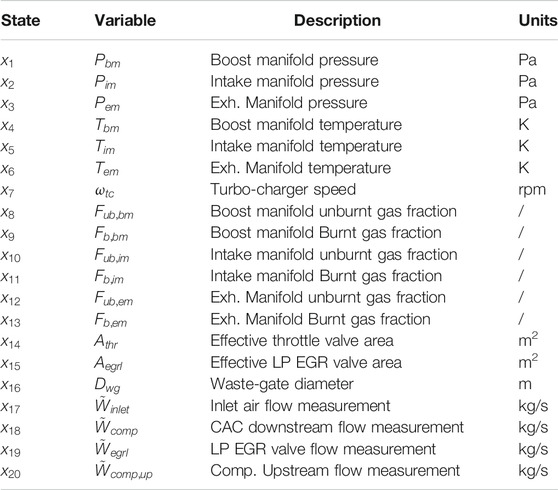
TABLE 2. State variables for the engine model.

TABLE 3

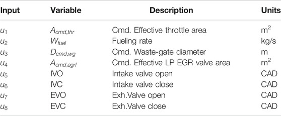
TABLE 3. Input variables for the engine model.

TABLE 4

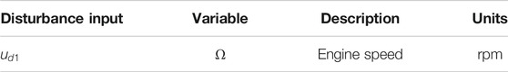
TABLE 4. Disturbance input variables for the engine model.

Taking the actuator and sensor response times into consideration, states $x_{14}$ to $x_{20}$ are added. First-order actuator responses are considered for the throttle valve, LP EGR valve and waste-gate. The following first-order approximation is used for the actuator and sensor dynamics:

$\dot{x}=\frac{x_0-x}{\tau }(17)$

where $x_0$ is the command actuator input or physical expressions of sensed variables without delay, and τ is the time constant.

In this engine model, the valve mass flow rate outputs are modeled by the following orifice equation (Eriksson and Nielsen, 2014):

$\begin{array}{l}W=A_{eff}\frac{P_{in}\sqrt{\gamma }}{\sqrt{R{T}_{in}}}f\left(\frac{P_{out}}{P_{in}}\right)\\ f\left(\frac{P_{out}}{P_{in}}\right)=\{\begin{array}{c}\sqrt{\frac{2}{\gamma -1}\left[{\left(\frac{P_{out}}{P_{in}}\right)}^{\frac{2}{\gamma }}-{\left(\frac{P_{out}}{P_{in}}\right)}^{\frac{\gamma +1}{\gamma }}\right]}\\ if\left(\frac{P_{out}}{P_{in}}\right)\ge {\left(\frac{2}{\gamma +1}\right)}^{\frac{\gamma }{\gamma -1}}\\ \sqrt{{\left(\frac{2}{\gamma +1}\right)}^{\frac{\gamma +1}{\gamma -1}}}\\ if\left(\frac{P_{out}}{P_{in}}\right)\le {\left(\frac{2}{\gamma +1}\right)}^{\frac{\gamma }{\gamma -1}}\end{array}\end{array}(18)$

where γ is the gas specific heat ratio, $A_{eff}$ is the effective valve area, $P_{out}$ is the downstream pressure, $P_{in}$ and $T_{in}$ are the upstream pressure and temperature. A virtual flow sensor, which is developed based on speed-density equation, can be used for estimating the cylinder charge flow rate. Figure 2 shows the comparison of the linear model estimated charge mass flow rate and the GT-Power reference. The maximum error for the virtual flow sensor is within ±5.1%.

FIGURE 2

FIGURE 2. Engine cylinder charge flow rate estimation.

The nonlinear model is linearized at the steady-state $\left(x_e,u_e,u_{de},y_e\right)$ of 3200 rpm engine speed, 60° throttle valve angle, 11.6 mm waste-gate diameter and 10° LP EGR valve angle. All of the valves are butterfly valves. The equilibrium points of system states x₁ to x₂₀ are directly obtained from GT-Power simulation results.

The nominal model is linearized into the following format:

$\begin{array}{l}\dot{x}=A\delta x+B\delta u+B_d\delta u_d\\ \delta y=C\delta x+D\delta u+D_d\delta u_d\end{array}(19)$

where $\delta x=x-x_e$, $\delta u=u-u_e$, $\delta u_d=u_d-u_{de}$, $\delta y=y-y_e$.

An observer is designed from the linear state-space model as follows. The state-space representation is a well-known practice to capture the system dynamics for its effective computation and real-time implementation. The observer is a linear dynamic system to correct the model estimation errors from measurements of the inputs and outputs of the real system.

$\begin{array}{l}\dot{\widehat{x}}=A\delta \widehat{x}+B\delta u+B_d\delta u_d+L\left(\delta y-\delta \widehat{y}\right)\\ \delta \widehat{y}=C\delta \widehat{x}+D\delta u+D_d\delta u_d\end{array}(20)$

In simulation results that follow, the commanded engine throttle angle and number of firing cylinders are fixed as their linearization points. As studied in Rivas Perea (2016), a 11.5% brake˗specific fuel consumption (BSFC) reduction and 4.5% absolute indicated efficiency improvement can be achieved by introducing 10% cooled EGR in a 2L, 4-cylinder, turbo-charged, direct injected SI engine at 3000 RPM part load conditions. Considering the fact that EGR tolerance decreases with the increasing engine speed (Francqueville and Michel, 2014), for an engine operation speed range of 2,400–4000 RPM, the waste-gate and LP EGR valve are operated as shown in Figure 3, to vary the EGR ratio within 1.5–11%, which is a helpful level for the SI engine to improve fuel efficiency and keep combustion stability. Figure 4 shows the indicated mean effective pressure (IMEP) of the engine for the drive cycle (per Figure 3), which demonstrates the implementation of the proposed sensor selection algorithm for medium/high-speed operating conditions.

FIGURE 3

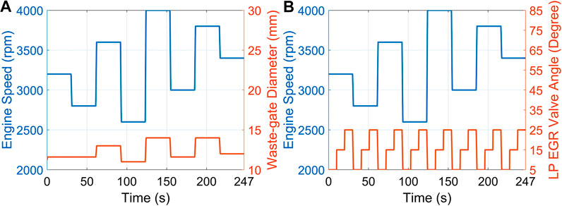
FIGURE 3. Engine operation conditions (A): engine speed and waste-gate (B): engine speed and LP EGR valve.

FIGURE 4

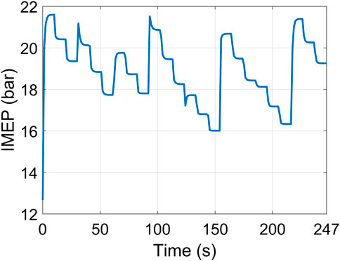
FIGURE 4. Engine operation conditions: engine IMEP.

3.2 Unknown Disturbance

The process noise $B_{w}w$ and measurement noise $Hv$ (per Eq. 1) are two necessary parameters to describe model and sensor errors. Incorrect description of the noise could result in significant worsening of estimation performances (Duník et al., 2017) and even the failure of the proposed sensor selection framework. Typically, the noise error covariance can be estimated by experimental tuning or computational methods (Duník et al., 2017; Kost et al., 2018; Solonen et al., 2014; Miran et al., 2019). The purpose of this section is to provide a simple and quick noise estimation method for the engine system based on experimental data to avoid repeated tuning work or complex computations. The sensor selection framework works well for the engine system with the diagonal noise covariance matrix estimated by the proposed method.

To implement the proposed sensor selection algorithm, the actual system is expressed as a linear state-space model with uncertainty represented by additive errors:

$\dot{x}=\delta \dot{x}=A\delta x+B\delta u+B_d\delta u_d+B_{w}w(21)$

where w is zero-mean unitary white noise and $B_w^T{B}_w$ is the process noise covariance matrix. The unknown disturbance $B_{w}w$ comes from the un-captured dynamics and model linearization errors. In this application, $B_w$ is assumed to be an diagonal matrix.

The modeling error $B_{w}w$ is estimated by fitting the difference between the actual $\dot{x}$ and the linear model estimated $\dot{x}$ as follows:

$B_{w}w={\dot{x}}_{GT}-\left(A\delta x_{GT}+B\delta u_{GT}+B_d\delta u_{d,GT}\right)=\Delta {\dot{x}}_{\mathrm{mod}el}(22)$

where the values of the variables ($\delta x_{GT}$, $\delta u_{GT}$, $\delta u_{d,GT}$) are from the GT-Power simulation result which is used as the truth-reference, and ${\dot{x}}_{GT}$ is the derivative of $x_{GT}$.

Figures 5–7 show the unknown disturbance plots for boost manifold pressure x₁, exhaust manifold pressure x₃ and turbocharger speed x₇, respectively. The errors $\Delta {\dot{x}}_{\mathrm{mod}el,1}$, $\Delta {\dot{x}}_{\mathrm{mod}el,3}$, and $\Delta {\dot{x}}_{\mathrm{mod}el,7}$ are calculated based on Eq. 22 where the data of states $x_{GT}$, inputs $u_{GT}$ and disturbance inputs $u_{d,GT}$ directly comes from the GT-Power simulation result for the drive cycle in Figure 3.

FIGURE 5

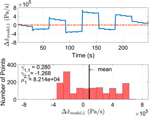
FIGURE 5. Unknown disturbance estimation for boost manifold pressure: $\text{Δ}{\dot{x}}_{model,1}$.

FIGURE 6

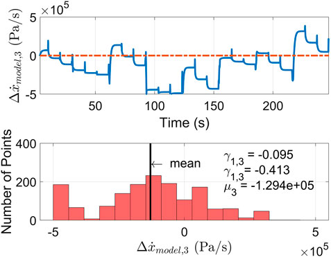
FIGURE 6. Unknown disturbance estimation for exhaust manifold pressure: $\text{Δ}{\dot{x}}_{model,3}$.

FIGURE 7

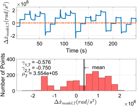
FIGURE 7. Unknown disturbance estimation for turbocharger speed: $\text{Δ}{\dot{x}}_{model,7}$.

An initial estimation of the process noise is the standard deviation of $\Delta {\dot{x}}_{\mathrm{mod}el}$ in Eq. 22. Considering the fact that non-normal noise (e.g. heavy-tailed or asymmetric) may not be well-represented by the first two moments (the mean and the standard deviation) Kost et al. (2018), the initial estimated process noise is then tuned based on its higher moments, i.e., skewness and kurtosis, to better represent the modeling errors.

3.2.1 Skewness Correction for Unknown Disturbance Estimation

The skewness ${\gamma }_1$ of the error $\text{Δ}{\dot{x}}_{model}$ is first calculated as follows to evaluate the asymmetry of the distribution and determine which $B_w\left(i,i\right)$ estimation equation is used for each state:

${\gamma }_{1,i}=\frac{\frac{1}{N}{\displaystyle {\sum }_{k=1}^N\left(\Delta {\dot{x}}_{\mathrm{mod}el,i}\left(k\right)-{\mu }_i\right)}}{{\sigma }_i^3}(23)$

where ${\mu }_i$ and ${\sigma }_i$ are the mean value and the standard derivation of $\text{Δ}{\dot{x}}_{model,i}$, respectively. ${\mu }_i$ and ${\sigma }_i$ are defined as follows:

$\begin{array}{l}{\mu }_i=\frac{1}{N}{\displaystyle \sum _{k=1}^N\Delta {\dot{x}}_{\mathrm{mod}el,i}\left(k\right)}\\ {\sigma }_i=\sqrt{\frac{1}{N}{\displaystyle \sum _{k=1}^N{\left(\Delta {\dot{x}}_{\mathrm{mod}el,i}\left(k\right)-{\mu }_i\right)}^2}}\end{array}(24)$

where N is the number of sampled points.

The positive skewness values mean that the data is skewed to the right (right-tail), and negative values suggest skewing to the left (left-tail) (Blanca et al., 2013). The larger the absolute skewness value is, the more significant the asymmetry is. For the states where the error $\text{Δ}{\dot{x}}_{model,7}$ has small skewness (per Figure 6), the asymmetry is neglected and the unknown disturbance term $B_w\left(i,i\right)$ is estimated by the following equation:

$B_w\left(i,i\right)=\sigma \left(i\right)(25)$

For the states where the error $\Delta {\dot{x}}_{\mathrm{mod}el,i}$ distributions have large skewness, the asymmetry should not be neglected when estimating the unknown disturbance. If the skewness ${\gamma }_{1,i}$ and the mean value ${\mu }_i$ have the same sign, the unknown disturbance of the state $x_i$ is estimated by the subtraction of the standard deviation ${\sigma }_i$ and the absolute mean value ${\mu }_i$ (per Figure 5), otherwise the unknown disturbance is estimated by the sum (per Figure 7). The condition in Eq. 26 is to account for both of the asymmetry and non-zero mean error distributions. For instance, if the mean is positive and the skewness is negative (per Figure 7), the error has a positive bias and the majority of the error are even more positive than the bias. In this situation, the standard deviation may under-estimate the error effect and thus we re-evaluate by adding the positive bias.

$B_w\left(i,i\right)={\sigma }_i-\left|{\mu }_i\right|if{\gamma }_{1,i}{\mu }_i>0(\mathrm{26a})$

$B_w\left(i,i\right)={\sigma }_i+\left|{\mu }_i\right|if{\gamma }_{1,i}{\mu }_i<0(\mathrm{26b})$

3.2.2 Kurtosis Correction for Unknown Disturbance Estimation

The excess kurtosis ${\gamma }_2$ of the error $\text{Δ}{\dot{x}}_{model}$ distribution defined as follows is then calculated to evaluate the outliers of the distribution and determine the correction made to the $B_w\left(i,i\right)$ term:

${\gamma }_{2,i}=\frac{\frac{1}{N}{\displaystyle {\sum }_{k=1}^N{\left(\Delta {\dot{x}}_{\mathrm{mod}el,i}\left(k\right)-\mu \left(i\right)\right)}^4}}{{\sigma }_i^4}-3(27)$

For the states which have negative excess kurtosis, the unknown disturbances have more data distributed outside the region of the peak than a normal distribution. The more negative the excess kurtosis is, the more outliers the distributions will have. When the excess kurtosis is large, Eqs 25, 26 without considering the extreme error distributions may not be a proper way to estimate the unknown disturbance. Therefore, a correction is made to the unknown disturbance estimations of the states which have excess kurtosis lower than $-1$ (per Figure 5) by the following equation:

$B_w\left(i,i\right)=B_{w0}\left(i,i\right)\left|{\gamma }_{2,i}\right|(28)$

where $B_{w0}$ is the modeling error estimated by Section 3.2.1.

For the states $x_{14}$ to $x_{20}$ which represent the delayed actuator and sensor responses, the unknown disturbance terms $B_w\left(i,i\right)$ are set as 0. The details of $B_w\left(i,i\right)$ estimation for each state is listed in Supplemental Material.

3.3 Measurement Noise

The diagonal measurement noise covariance matrix H is defined as:

$H=\left[\begin{array}{cccc}4\%\delta W_{inlet,\max }& 0& 0& 0\\ 0& 2\%\delta W_{comp,\max }& 0& 0\\ 0& 0& 7\%\delta W_{egrl,\max }& 0\\ 0& 0& 0& 4\%\delta W_{comp,up,\max }\end{array}\right](29)$

where sensor accuracy data comes from Table 1 and $\delta W_{max}$ is the maximum flow rate deviation with respect to its linearization point.

3.4 Sensor Selection Results

The sensor selection algorithm is applied to the scaled linear system. This is to eliminate the effect of magnitude differences of measurements.

Table 5 shows the optimal sensor set computed by the sensor selection algorithm (per Section 2) for different sensor number constraints. The iterative parameter ɛ is set as $1e^{-3}$ for single and two-sensor combinations or $1.2e^{-2}$ for three-sensor combinations. The trace(T), representing the upper power bound of the expected estimation RMSE, is calculated by Eq. 15 when setting $\alpha =0$ for the normalized system. The upper bound of the expected RMSE $\mathcal{E}{\left\{RMSE\right\}}_{ub}$ and the expected RMSE $\mathcal{E}\left\{RMSE\right\}$ for the actual system can be expressed, and related as follows:

$\begin{array}{l}\mathcal{E}{\left\{RMSE\right\}}_{ub}\ge \mathcal{E}\left\{RMSE\right\}\\ \mathcal{E}{\left\{RMSE\right\}}_{ub}=\delta x_{11,\max }\sqrt{trace\left(T\right)}\\ \mathcal{E}\left\{RMSE\right\}=\delta x_{11,\max }\sqrt{trace\left({\left({\tilde{B}}_w-L\tilde{H}\right)}^{T}P\left({\tilde{B}}_w-L\tilde{H}\right)\right)}\end{array}(30)$

where $\delta x_{11,max}=max\left(x_{11}-x_{e,11}\right)$ is the scaling parameter of the intake manifold burnt gas fraction $x_{11}$. It can be noticed that $\mathcal{E}{\left\{RMSE\right\}}_{ub}$ is a very tight upper bound of $\mathcal{E}\left\{RMSE\right\}$ for this application as shown in Table 5.

TABLE 5

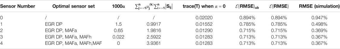
TABLE 5. Sensor selection results.

The algorithm identifies the EGR DP sensor as the best sensor if only one single can be used. When two sensors are used, the optimal sensor set becomes EGR DP and MAFa, which measures the inlet air mass flow rate before the EGR joint (per Figure 1). The optimal three-sensor set combines EGR DP, MAFa and MAFh.

Different sensor sets with their corresponding observers are tested on the reference engine model in GT-Power. The four candidate sensors (per Table 1 and Figure 1) are placed in the GT-Power model. Per Table 1 data, these four GT-Power outputs are filtered with first-order functions described in Eq. 17 and corrupted by measurement noise before being sent to the observers to account for sensor noise. The GT-Power and observer simulation structure is shown in Figure 8. The observer gain for each sensor set is computed by the optimization (15) with $\alpha =0$. The real-time inputs of the engine actuators (per Table 3 and the engine speed are known to the observer. The GT-Power cycle-averaged intake manifold burnt gas fraction is used as the truth-reference to validate the estimation results. RMSE of the intake manifold burnt gas mass fraction estimation for each sensor set is calculated from 3.3s to the end of the simulation to eliminate the effects of initial conditions.

FIGURE 8

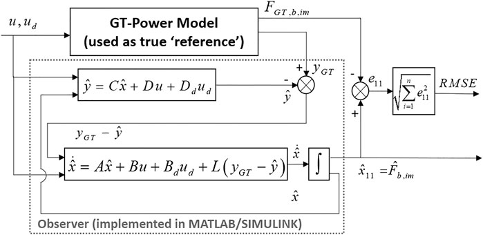
FIGURE 8. Diagram of GT-Power and observer simulation structure.

3.4.1 Single Sensor Sets

Figure 9 shows the estimation results of intake manifold burnt gas mass fraction when using different single sensor sets. As shown in Figure 9A, the EGR DP sensor has the most accurate estimation results at every step. Considering the overall estimation performance, the EGR DP sensor is the most accurate single-sensor option since it has the smallest root-mean-square error (RMSE), 0.498%, over the entire simulation. Without using any sensor, the maximum absolute estimation error is 1.744%. With the computed optimal sensor EGR DP, the maximum error is reduced to 1.014%, which is a 42% improvement compared to the model-only estimated result. The maximum errors for single MAFa sensor, MAFh sensor and MAF sensor are 1.684, 1.724 and 1.724%, respectively. Figure 9B shows the transient tracking performance of intake manifold burnt gas mass fraction when using different single sensor sets. Per Figure 9B, EGR DP sensor has the best tracking performance during the transient change. MAFa sensor is slightly better than MAFh sensor and MAF sensor. Even though the upstream compressor flow sensor MAF has a shorter response time than the downstream compressor flow sensor MAFh (per Table 1), there is few difference between the tracking transient performance of these two sensors (per Figure 9B).

FIGURE 9

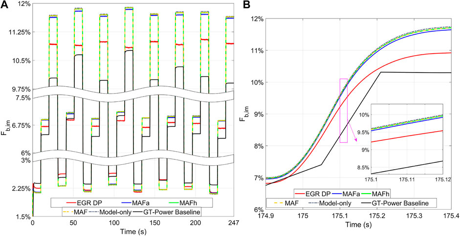
FIGURE 9. Intake manifold burnt gas mass fraction estimation when only using one sensor (A): the entire drive cycle (B): transient performance (500 ms zoomed).

As shown in Table 6, the RMSE for a single MAFa sensor, a single MAFh sensor and a single MAF sensor are 0.909, 0.935 and 0.935%, respectively. This indicates that if the EGR DP sensor fails, the next sensor the engine should select is the MAFa sensor based on their trace (T) and $\mathcal{E}{\left\{RMSE\right\}}_{ub}$ calculations. Though the MAFh sensor has slightly lower trace (T) and $\mathcal{E}{\left\{RMSE\right\}}_{ub}$ than the MAF sensor, their estimation performances are the same.

TABLE 6

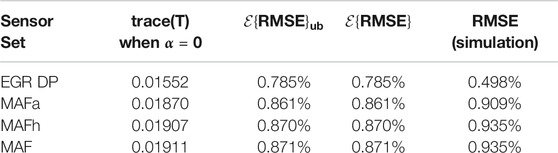
TABLE 6. Single sensor set.

Figure 10 shows the histograms of different single sensor sets’ estimation errors. Compared to the optimal sensor EGR DP, the error distributions of the other three sensors are more spread out.

FIGURE 10

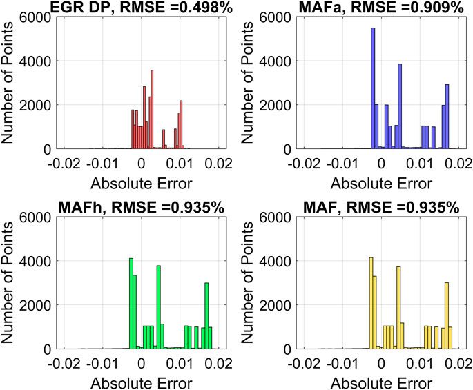
FIGURE 10. Histograms of Intake manifold burnt gas mass fraction estimation error when only using one sensor.

3.4.2 Two-Sensor Sets

The optimal two-sensor set computed by the sensor selection algorithm (per Section 2) is the combination of the EGR DP and MAFa sensors. This is verified in the coupled GT-Power/Observer simulation (per Figure 8). As shown in Figure 11, the computed optimal sensor set has the smallest estimation error for almost every step. Comparing the overall estimation performance of the optimal sensor set with the other five combinations, the optimal one has the lowest RMSE. With the computed optimal sensor set, the maximum error is reduced to 0.754%, which is 57% improvement compared to the model estimated result. The maximum estimation error is 0.794% for the combination of EGR DP sensor and upstream compressor flow sensor MAFh, and is 0.804% for the combination of EGR DP sensor and downstream compressor flow sensor MAF. For the combinations of MAFa sensor + MAFh sensor, MAFa sensor + MAF sensor, the maximum estimation errors are both 1.564 and 1.594%. When only two compressor flow sensors are used, the maximum error is up to 1.724%.

FIGURE 11

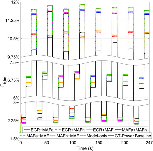
FIGURE 11. Intake manifold burnt gas mass fraction estimation when using two sensors.

In Table 7 and Figure 12, the simulated RMSE for different two-sensor set combinations monotonically increases with increasing $\mathcal{E}\left\{RMSE\right\}$, as expected. The sensor sets with the first three lowest $\mathcal{E}\left\{RMSE\right\}$ all include the EGR DP sensor. Though the algorithm computes the combination of EGR DP sensor and MAFa sensor as the optimal two-sensor set, the combination of EGR DP sensor + MAFh sensor and EGR DP sensor + MAF sensor have similar estimation performances as the optimal one, as shown in Figure 11. These two combinations have very close $\mathcal{E}\left\{RMSE\right\}$ as well as the RMSE as shown in Table 7. When EGR DP is not considered in the two-sensor combination, such as the combination of MAFa sensor and MAFh sensor, there is a large increase in $\mathcal{E}\left\{RMSE\right\}$ as well the simulated RMSE. Additionally the two-sensor sets without the EGR DP sensor even have larger estimation errors than single EGR DP sensor. This indicates that under this operation condition, if only two sensors are allowed, the combination should include EGR DP sensor, and an EGR DP-only strategy would be preferred over a two-sensor strategy which did not include the EGR DP sensor. The optimal selection of the sensor in addition to the EGR DP sensor is MAFa sensor. The MAFh sensor may be considered as a backup selection to the MAFa sensor.

TABLE 7

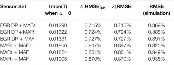
TABLE 7. Two-sensor combinations.

FIGURE 12

FIGURE 12. RMSE vs. trace(T) for two-sensor combinations.

Figure 13 shows the histograms of different two-sensor combinations estimation errors. As shown, the best three two-sensor combinations have the estimation errors distributions closer to 0.

FIGURE 13

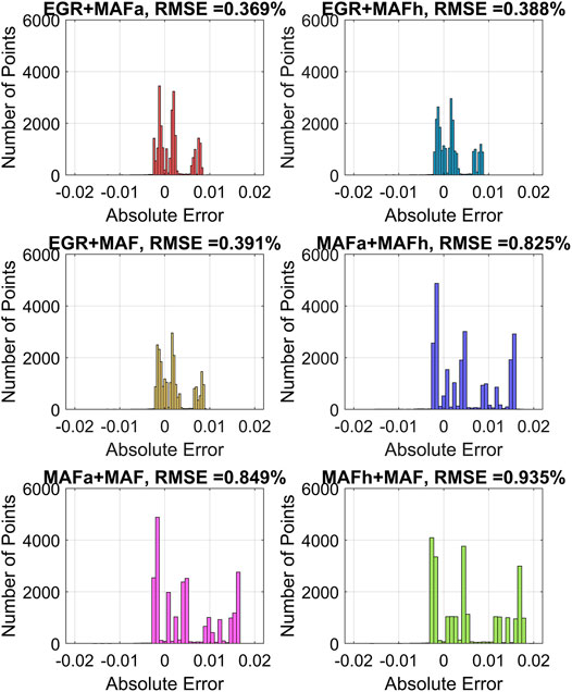
FIGURE 13. Histograms of intake manifold burnt gas mass fraction estimation error when using two sensors.

3.4.3 Optimal Sensor Sets

Figure 14 show the estimation results of intake manifold burnt gas mass fraction $F_{b,im}$ when using optimal sensor sets with different sensor numbers. As shown in Figure 14, the optimal two-sensor set has better estimation performance than the optimal single sensor. When more than two sensors can be used, all the optimal sensor set options have very similar estimation performances. Based on the data shown in Table 5, the optimal single sensor EGR DP reduces the RMSE by 47.4% compared with model-only estimated results. The optimal two-sensor option further reduces the RMSE by 25.9% based on the optimal single sensor estimation performance. Comparing the RMSE of the optimal three-sensor set, 0.367%, with the RMSE of the optimal two-sensor set, 0.369%, there is only 0.5% accuracy improvement. When the fourth sensor is added to the optimal three-sensor set, there is no improvement for the RMSE. In Figure 15, the computed $\mathcal{E}\left\{RMSE\right\}$ and trace(T) have similar trends. Using the optimal single sensor reduces the tarce(T) by 23.2% and $\mathcal{E}\left\{RMSE\right\}$ by 12.2% compared with model-only estimation results. From the optimal single sensor to the optimal two-sensor set, the trace(T) and $\mathcal{E}\left\{RMSE\right\}$ have 16.9 and 8.9% reductions, respectively. From the optimal two-sensor set to the optimal three-sensor set, the trace(T) is only lowered by 0.5% and $\mathcal{E}\left\{RMSE\right\}$ is lowered by 0.3%. From the optimal three-sensor set to the all-sensor set, both trace(T) and $\mathcal{E}\left\{RMSE\right\}$ remain the same. Compare the trends of $\mathcal{E}\left\{RMSE\right\}$ (or trace(T)) and simulated RMSE, both $\mathcal{E}\left\{RMSE\right\}$ (or trace(T)) and simulated RMSE have relative large reductions from model-only case to single sensor case to two-sensor case and small decreases when adding the third or fourth sensor. In this way, $\mathcal{E}\left\{RMSE\right\}$ or trace(T) can be a useful indicator of showing the necessity or redundancy when adding additional sensors.

FIGURE 14

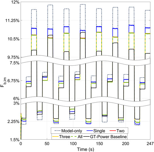
FIGURE 14. Intake manifold burnt gas mass fraction estimation when using optimal sensor sets.

FIGURE 15

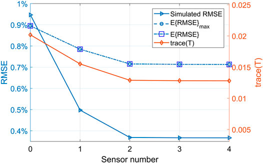
FIGURE 15. RMSE and trace(T) vs. sensor number for optimal sensor sets.

The sensor selection results indicates that though increasing sensor number reduces RMSE, the added sensor(s) brings in very small improvements of the estimation performance when number of sensors is higher than two. Based on the estimation error requirement, it may be worth using a single EGR DP sensor or adding a second sensor MAFa in addition to a single EGR DP sensor, but it may not be worth spending more money on adding the third or fourth sensor for the intake manifold gas composition estimation.

Figure 16 shows the histograms of different optimal sensor combinations estimation errors. It can be seen that with the increasing of sensor number, the RMSE distribution is narrowed down and has smaller peaks at large errors.

FIGURE 16

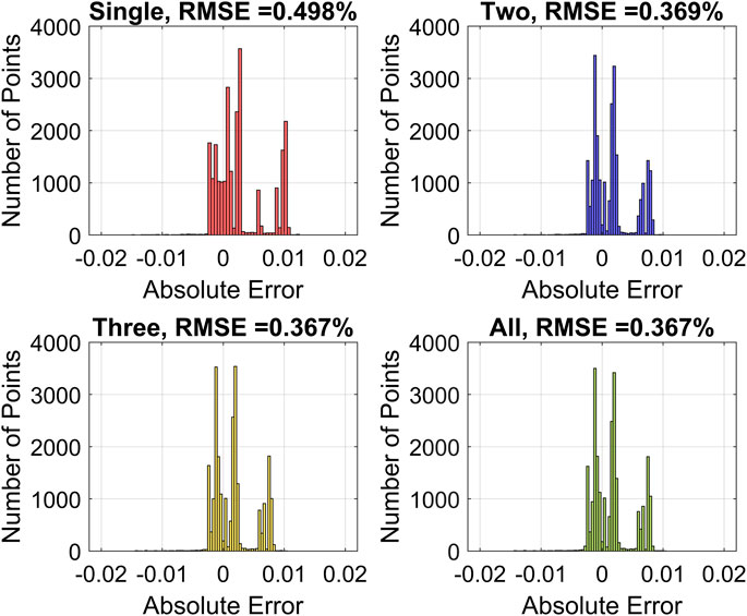
FIGURE 16. Histograms of intake manifold burnt gas mass fraction estimation error when using optimal sensor sets.

3.4.4 Additional Discussion

The difference between the expected RMSE $\mathcal{E}\left\{RMSE\right\}$ and the simulated RMSE is shown in Tables 5–7, as well as Figures 12, 15. This could be explained by: (i) The computation of the expected RMSE, $\mathcal{E}\left\{RMSE\right\}$ (via Eq. 24), is based on the assumption that the process noise is zero-mean white noise. However, the actual unknown disturbance term ${\dot{x}}_{GT}$ is not normally distributed for the example testing cycle. Since this paper focusing on selecting the optimal sensor set among candidate sensors for the engine system rather than studying the differences between the engine model and actual system, a quick and simple approximation method of the process noise described in Section 3.2 was used. The valuable information provided by the sensor selection algorithm is the sequence and relative increase/decrease among different sensor sets. Further studies could focus on a more appropriate unknown disturbance estimation method, but this would not be expected to change the sensor selection results and thus was not the study purpose; (ii) The measurement noise is approximated by the product of the maximum deviation of the sensor measurement with respect to its linearization point and the accuracy (per Section 3.3). This simple approximation would result in some differences between the expected RMSE $\mathcal{E}\left\{RMSE\right\}$ and the simulated RMSE due to the reason that the actual sensor measurement deviations are not symmetric about the linearization points, but would not be expected to change the sensor selection results. Further studies could focus on a more appropriate measurement noise estimation method based on analytical approaches.

4 Conclusion

This paper outlines a sensor selection and observer deign algorithm based on H₂ optimization while considering process and measurement noise. The approach is (1) implemented to an advanced turbo-charged spark-ignited engine architecture using exhaust gas circulation; and (2) validated on a high fidelity engine simulation in GT-Power. The objective of the sensor selection + observer design algorithm is to minimize the estimation error and the required sensor numbers. The optimization problem is convexified and solved via SDP. A method to estimate the unknown model uncertainties was also developed. The high fidelity simulation results verified that the optimal sensor sets computed by the algorithm had the best estimation performances. Sensor redundancy was also analyzed based on the computation results. This algorithm reduces the computation time and experimental efforts of selecting optimal sensor sets.

5 Future Work

The future work of this algorithm study can involve the estimation of other engine key parameters and observer designs; other engine operation conditions analysis.

Data Availability Statement

The raw data supporting the conclusion of this article will be made available by the authors, without undue reservation.

Author Contributions

XZ and GS developed the theory, performed the computations and planned the simulations. XZ carried out the simulations. XZ and GS wrote the manuscript with support from CL, DG, and DaL. DL supervised the project.

Conflict of Interest

CL, DG, DaL and DL were employed by the company Cummins Inc.

The remaining authors declare that the research was conducted in the absence of any commercial or financial relationships that could be construed as a potential conflict of interest.

Acknowledgments

This material is based upon work supported by the U.S. Department of Energy.

Supplementary Material

The Supplementary Material for this article can be found online at: https://www.frontiersin.org/articles/10.3389/fmech.2021.611992/full#supplementary-material.

References

Arzelier, D. (2008). “LMIs in systems control state-space methods performance analysis and synthesis”, in Lecture Notes of LAAS course on LMIs optimization with application in control Part II.

Google Scholar

Blanca, M. J., Arnau, J., López-Montiel, D., Bono, R., and Bendayan, R. (2013). Skewness and kurtosis in real data samples. Methodol. Eur. J. Res. Methods Behav. Soc. Sci. 9, 78–74. doi:10.1027/1614-2241/a000057

CrossRef Full Text | Google Scholar

Candes, E. J., Wakin, M. B., and Boyd, S. P. (2008). Enhancing sparsity by reweighted minimization. J. Fourier Anal. Appl. 14, 877–905. doi:10.1007/s00041-008-9045-x

CrossRef Full Text | Google Scholar

Chen, P., and Wang, J. (2012). Oxygen concentration dynamic model and observer-based estimation through a diesel engine aftertreatment system. J. Dyn. Syst. Meas. Control. 134, 031008. doi:10.1115/1.4005508

CrossRef Full Text | Google Scholar

Chepuri, S. P., and Leus, G. (2014). Sparsity-promoting sensor selection for non-linear measurement models. IEEE Trans. Signal Process. 63, 684–698. doi:10.1109/TSP.2014.2379662

CrossRef Full Text | Google Scholar

Chong, E. K., and Zak, S. H. (2013). An introduction to optimization, 4th Edn. Vol. 76. Hoboken, NJ: John Wiley & Sons.

Dhingra, N. K., Jovanović, M. R., and Luo, Z.-Q. (2014). “An ADMM algorithm for optimal sensor and actuator selection,” in 53rd IEEE conference on decision and control (IEEE), Los Angeles, CA, 15–17 Dec. 2014 (IEEE), p. 4039–4044.

Google Scholar

Duník, J., Straka, O., Kost, O., and Havlík, J. (2017). Noise covariance matrices in state-space models: A survey and comparison of estimation methods-Part I. Int. J. Adapt Control. Signal. Process. 31, 1505–1543. doi:10.1002/acs.2783

CrossRef Full Text | Google Scholar

Eriksson, L., and Nielsen, L. (2014). Modeling and control of engines and drivelines. 1st edn, Hoboken, NJ: John Wiley & Sons.

CrossRef Full Text

Fardad, M., Lin, F., and Jovanović, M. R. (2011). “Sparsity-promoting optimal control for a class of distributed systems,” in Proceedings of the 2011 American control conference, San Francisco, CA. 29 June–1 July 2011 (IEEE).

CrossRef Full Text | Google Scholar

Francqueville, L., and Michel, J.-B. (2014). On the effects of egr on spark-ignited gasoline combustion at high load. SAE Int. J. Eng. 7, 1808–1823. doi:10.4271/2014-01-2628

CrossRef Full Text | Google Scholar

Grant, M. C., and Boyd, S. P. (2015). The CVX users™ guide release, 2.1. Austin, TX: CVX Research Inc.,

Hashemi, A., Ghasemi, M., Vikalo, H., and Topcu, U. (2018). “A randomized greedy algorithm for near-optimal sensor scheduling in large-scale sensor networks,” in 2018 Annual American control conference. (ACC), Milwaukee, WI, 27–29 June 2018 (IEEE), p. 1027–(1032.).

Google Scholar

Joshi, S., and Boyd, S. (2008). Sensor selection via convex optimization. IEEE Trans.Signal Process. 57, 451–462. doi:10.1109/TSP.2008.2007095

CrossRef Full Text | Google Scholar

Kalandros, M., and Pao, L. Y. (1998). “Controlling target estimate covariance in centralized multisensor systems,” in Proceedings of the 1998 American control conference ACC (IEEE Cat. No. 98ch36207) (IEEE), Philadelphia, PA, 26–26 June 1998, 2749–2753.

Google Scholar

Kalandros, M., Pao, L. Y., and Ho, Y.-C. (1999). “Randomization and super-heuristics in choosing sensor sets for target tracking applications,” in Proceedings of the 38th IEEE conference on decision and control (cat No. 99CH36304) (IEEE), Phoenix, AZ, 7–10 Dec. 1999, 2, 1803–1808.

Google Scholar

Kocher, L., Koeberlein, E., Van Alstine, D., Stricker, K., and Shaver, G. (2012). Physically based volumetric efficiency model for diesel engines utilizing variable intake valve actuation. Int. J. Eng. Res. 13, 169–184. doi:10.1177/1468087411424378

CrossRef Full Text | Google Scholar

Kost, O., Duník, J., and Straka, O. (2018). Noise moment and parameter estimation of state-space model. IFAC-POL 51, 891–896. doi:10.1016/j.ifacol.2018.09.107

CrossRef Full Text | Google Scholar

Luo, Z.-Q., Chang, T.-H., Palomar, D., and Eldar, Y. (2010). SDP relaxation of homogeneous quadratic optimization: approximation. Convex Optimi. Signal. Process. Commun. 117. doi:10.1017/CBO9780511804458.005

Google Scholar

Miran, S., Simon, J. Z., Fu, M. C., Marcus, S. I., and Babadi, B. (2019). “Estimation of state-space models with Gaussian mixture process noise,” in 2019 IEEE Data Science Workshop (DSW), Minneapolis, MN, 2–5 June 2019 (IEEE).

CrossRef Full Text | Google Scholar

Münz, U., Pfister, M., and Wolfrum, P. (2014). Sensor and actuator placement for linear systems based on and optimizationsensor and actuator placement for linear systems based on H₂ and H_∞ optimization. IEEE Trans. Automat. Contr. 59, 2984–2989. doi:10.1109/tac.2014.2351673

CrossRef Full Text | Google Scholar

Mushini, R., and Simon, D. (2005). “On optimization of sensor selection for aircraft gas turbine engines,” in 18th international conference on systems engineering (ICSEng’05), Las Vegas, NV, 16–18 Aug. 2005, 9–1.

Google Scholar

Palmer, K. A., Hale, W. T., and Bollas, G. M. (2018). “Active fault diagnosis with sensor selection in a diesel engine air handling system,” in 2018 Annual American control conference (ACC), Milwaukee, WI, 27–29 June 2018 (IEEE), 4995–(5000.)

Google Scholar

Peet, M. M. (2016). LMI methods in optimal and robust control. Lecture Notes, Department of Mechanical and Aerospace Engineering ((Tempe, AZ: Arizona State University).

Google Scholar

Pekař, J., Garimella, P., Germann, D., and Stewart, G. E. (2012). Experimental results for sensor selection and multivariable controller design for a heavy-duty diesel engine. IFAC Proc. Vol. 45, 122–129.

Google Scholar

Polyak, B., Khlebnikov, M., and Shcherbakov, P. (2013). “An LMI approach to structured sparse feedback design in linear control systems,” in 2013 European control conference (ECC). Zurich, 17–19 July 2013(IEEE), 833–838.

Google Scholar

Rao, S., Chepuri, S. P., and Leus, G. (2015). “Greedy sensor selection for non-linear models,” in 2015 IEEE 6th international workshop on computational advances in multi-sensor adaptive processing (CAMSAP). Cancun, CUN, 13–16 Dec. 2015 (IEEE), 241–244.

Google Scholar

Rengarajan, S. B., Sarlashkar, J., Roecker, R., and Anderson, G. (2018). Estimation of intake oxygen mass fraction for transient control of EGR engines, SAE Technical Paper, Tech. Rep.

CrossRef Full Text | Google Scholar

Rivas Perea, M. E. (2016). Assessment of fuel consumption reduction strategies on a gasoline turbocharged direct injection engine with a cooled EGR system. Ph.D. Thesis. Valencia, Spain Universitat Politècnica de València.

Google Scholar

Simon, D. L., and Garg, S. (2010). Optimal tuner selection for kalman filter-based aircraft engine performance estimation. J. Eng. Gas Turbin. Power 132. 031601‐1–031601‐10. doi:10.1115/1.3157096

CrossRef Full Text | Google Scholar

Solonen, A., Hakkarainen, J., Ilin, A., Abbas, M., and Bibov, A. (2014). Estimating model error covariance matrix parameters in extended kalman filtering. Nonlin. Process. Geophys. 21, 919–927. doi:10.5194/npg-21-919-2014

CrossRef Full Text | Google Scholar

Stricker, K., Kocher, L., Koeberlein, E., Van Alstine, D., and Shaver, G. M. (2014). Turbocharger map reduction for control-oriented modeling. J. Dyn. Syst. Meas. Control. 136, 041008. doi:10.1115/1.4026532

CrossRef Full Text | Google Scholar

Suard, R., Onder, C. H., and Guzzella, L. (2008). Optimal sensor selection and configuration, case study spark ignited engine. SAE Int. J. Passeng Cars Electron. Electr. Syst. 1, 382–392. doi:10.1109/tit.2005.864420

CrossRef Full Text | Google Scholar

Tropp, J. A. (2006). Just relax: convex programming methods for identifying sparse signals in noise. IEEE Trans. Inform. Theor. 52, 1030–1051. doi:10.1109/tit.2005.864420

CrossRef Full Text | Google Scholar

Van Alstine, D. G., Kocher, L. E., Koeberlein, E., Stricker, K., and Shaver, G. M. (2013). Control-oriented premixed charge compression ignition combustion timing model for a diesel engine utilizing flexible intake valve modulation. Int. J. Eng. Res. 14, 211–230. doi:10.1016/j.conengprac.2008.04.007

CrossRef Full Text | Google Scholar

Wang, J (2008). Air fraction estimation for multiple combustion mode diesel engines with dual-loop egr systems. Control. Eng. Pract. 16, 1479–1486. doi:10.1016/j.conengprac.2008.04.007

CrossRef Full Text | Google Scholar

Zare, A., and Jovanović, M. R. (2018). “Optimal sensor selection via proximal optimization algorithms,” in 2018 IEEE conference on decision and control (CDC), Miami Beach, MI, 17–19 Dec. 2018, 6514–(6518.) (IEEE).

Google Scholar