 Andreas Kainz1,2*
 Silvan Schmid
95% of researchers rate our articles as excellent or good
Learn more about the work of our research integrity team to safeguard the quality of each article we publish.
Find out more
ORIGINAL RESEARCH article
Front. Mech. Eng. , 19 February 2021
Sec. Micro- and Nanoelectromechanical Systems
Volume 6 - 2020 | https://doi.org/10.3389/fmech.2020.611590
This article is part of the Research Topic Nanomechanical Sensors View all 5 articles
With their unparalleled mass sensitivity, enabling single-molecule mass spectrometry, nanomechanical resonators have the potential to considerably improve existing sensor technology. Vertical pillar resonators are a promising alternative to the existing lateral resonator designs. However, one major obstacle still stands in the way of their practical use: The efficient transduction (actuation & detection) of the vibrational motion of such tiny structures, even more so when large arrays of such nanopillars need to be driven. While electrostatic forces are typically weak and, on the nanoscale even weaker when compared to a cantilever-like stiffness, it is worth revisiting the possibility of electrostatic actuation of nanomechanical pillars and other nanomechanical structures. In this paper, these forces produced by an external field are studied both analytically and numerically, and their dependencies on the geometric dimensions are discussed. Furthermore, the expected deflections for different configurations of pillar geometries are calculated and compared.
Microelectromechanical systems (MEMS) have become an integral part of modern consumer products and professional medical devices, and as such have become omnipresent helpers in our lives. As an example, there are more than one dozen MEMS parts contained in a modern smartphone alone, including gyroscopes, microphones, filters, switches, oscillators, accelerometers, auto focus actuators, electronic compass, pressure sensors, proximity sensors, fingerprint sensor, etc. The sensitivity and energy efficiency of micromechanical sensors typically improve with downscaling, which has led to the development of nanoelectromechanical systems (NEMS) with feature sizes below 1 μm in two dimensions. The first NEMS were developed at the end of the last century and consisted of nano-scale mechanical silicon-based resonators (Cleland and Roukes, 1996). The mechanical oscillations of such resonators are highly sensitive to perturbations coming from the environment. This makes them excellent sensors in particular for mass sensing, since the mass responsivity inversely scales with the effective mass of the resonator (Schmid et al., 2016). Carbon nanotube resonators with an ultimately low effective mass have reached yoctogram sensitivity (Chaste et al., 2012). Besides such fundamental research, nanomechanical resonators are promising for the application in protein (Naik et al., 2009; Hanay et al., 2012; Sage et al., 2015) or aerosol mass spectrometry (Schmid et al., 2013), offering, for the first time, single-molecule sensitivity. Despite the unparalleled mass sensitivity of nanomechanical resonators, their application as practical sensors has remained challenging. The typically used horizontal nanomechanical sensors are sensitive to the landing position of the mass along their length. This requires a sophisticated dual-mode operation of the first and second normal mode (Naik et al., 2009; Dohn et al., 2010; Schmid et al., 2010), which significantly complicates the sensor design. Vertical nanomechanical pillar resonators constitute a promising design alternative with all the advantages of having a low mass. And in contrast to horizontal resonator designs, the mass loading happens at the tip of the pillars which renders dual-mode operation unnecessary.
The efficient transduction (actuation & detection of mechanical motion) of NEMS has generally remained a challenge, for pillars in particular. Typical techniques used to transduce nanomechanical resonators, such as magnetomotive (Cleland and Roukes, 1996), piezoelectric (Villanueva et al., 2011), resistive (Li et al., 2007), and dielectric polarization-based (Schmid et al., 2006; Unterreithmeier et al., 2009; Faust et al., 2012) techniques are not well suited to transduce the vertical vibration of pillars. Optical detection of mechanical motion is the most sensitive technique available. Recently it was shown that the vibration of vertical nanowires can be readily detected optically (Molina et al., 2020). When the vertical nanowires are situated at the slope maximum of the Gaussian light beam, the displacement of the light-scattering nanowires cause a modulation of the reflected light. A similar method has been used to detect the lateral motion of nanoparticles situated inside a Gaussian beam (Chien et al., 2020). A different approach relevant for this paper is to produce pillar dimers (Sadeghi et al., 2017), which allow for a plasmonic optical readout as presented with nanomechancial string resonators (Thijssen et al., 2015).
The remaining challenge is how to efficiently drive such nanomechanical pillar dimers. With typical resonance frequencies >10 MHz the actuation with an external piezoelectric shaker becomes ineffective. In this paper, we propose to drive pillar dimers electrostatically by means of an external electrostatic field. We study the case of pillar dimers featuring a conductive tip, e.g., a plasmonic gold tip (Sadeghi et al., 2017), or pillars that are made of a conductive material, such as gold (Kabashin et al., 2009) (Figure 1). The generation of local forces between two electrically isolated floating electrodes via the application of an external electrostatic field constitutes an interesting transduction scheme for NEMS. Besides the here presented specific transduction scheme of conductive nanopillars, floating electrodes are often a given design constraint, e.g., in ultrahigh-Q string or drum resonators where a metalization of the entire resonator would significantly deteriorate the quality factor (Unterreithmeier et al., 2009; Yu et al., 2012; Bagci et al., 2014; Schmid et al., 2014). Hence, the presented analytical model is applicable beyond the transduction of nanomechancial pillar dimers, specific schemes for the transduction of string or nanowire resonators, as well as drum resonators, are promising extensions.
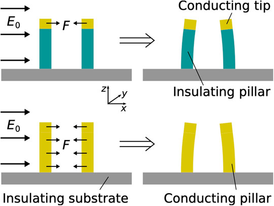
FIGURE 1. Working principle of the electrostatic pillar actuation. The applied electric field
In contrast to conventional electrostatic drives where a voltage is applied between a static and a moving electrode, we intend to exploit the polarisation of conductors inside an electric field. The polarisation then leads to surface charges on the conductor, which experience a force inside the electric field. A measurable deflection can be achieved by an elastic element between the oppositely charged surface regions, which can be used as electric field sensor (Kainz et al., 2018, Kainz et al., 2019).
While for a single uncharged conductor the total force after integration over the surface of the whole conductor is zero, a net force emerges when two or more such conductors are brought close to one another (Figure 1). For the estimation of this electrostatic force between two nanomechanical pillars, a pair of conducting bodies (spheres, discs, or cylinders) is placed inside a uniform electric field E.
In many applications, rigorous analytical representations cannot be achieved without significant simplifications that generally question the reliability of the utilized modelling approach. Numerical methods have become powerful tools capable of filling this gap. Furthermore, numerical results tend to obfuscate fundamental dependencies. Reasonable analytical modelling should always be preferred. Therefore, a benchmark case in order to compare the analytical and numerical results is necessary to find solver settings and mesh quality which allow accurate results with minimum computational power. In the case of dimers, it seems best suited to use two conducting spheres embedded inside a uniform electric field for this purpose, which we’ll be presented subsequently. Forces between two cylinders will be introduced afterwards.
The analytical treatment of the problem of two conducting spheres dates back at least to (Jenss, 1932) and (Morse and Feshbach, 1953). An extensive treatment of this case was done by (Davis, 1964). This quite general work is based on bispherical coordinates and treats conductive spheres of different sizes and charges, and varying distance in an electric field of arbitrary direction. Here, the resulting force for two uncharged spheres of the same radius r from this publication is used, considering only an electric field E0 parallel to the axis between these spheres (here the z-axis). The corresponding force for a distance d between the spheres acts in the same direction and is given in electrostatic units as
where
is an infinite sum with
The terms Yn can be written as
with
The terms
Note that this force corresponds to the force acting on one of the spheres.
The associated numerical model was built in COMSOL using the electrostatics module. The two spheres were embedded inside a uniform field generated by two parallel plates. To model them as perfect conductors a floating potential boundary condition was applied to each. The corresponding forces were obtained by integration of the radial component of the electrostatic stress tensor over the surface of one sphere.
For comparison, a sphere radius of
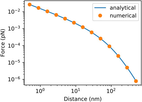
FIGURE 2. Comparison between analytically and numerically obtained forces between two uncharged conducting spheres of radius r = 50 nm in a uniform electric field with a field strength
Unfortunately, the problem of two nanopillars cannot be described analytically in the same quality as the two spheres, since certain assumptions and simplifications have to be made. By assuming infinitely long parallel cylinders oriented in z-direction, the three-dimensional problem can be reduced to a two-dimensional one. The top and bottom faces of the actually finite-sized cylinders (height L) are neglected.
The distance between the cylinders be denoted s, the radii by R1, R2. The distances between the center of a cylinder to the origin are given by D1 and D2, respectively (Figure 3). Therefore, the centre-to-centre distance between the cylinders is d = s + R1 + R2 = D1 + D2. The electric field is assumed to be oriented in x-direction, E0 =
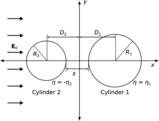
FIGURE 3. Cross-section of the two cylinders and important dimensions.
As for the bispherical problem, the bicylindrical problem can be treated analytically using a suitable coordinate system. Here, bipolar (BP) coordinates are a good choice for the 2D problem (Moon and Spencer, 1961). A solution for the electrostatic potential of two conducting cylinders in a uniform electric field has also been outlined in (Jenss, 1932; Morse and Feshbach, 1953). The most general treatment of the electrostatic two-cylinder problem has been presented in (Emets and Onofrichuk, 1996), however without using BP coordinates and without calculating the potential.
It pays off to perform the calculation of the potential by solving Laplace’s equation with the actual application in mind, which is outlined in the following. Cartesian (x, y) and BP (
For now, a can be regarded as an arbitrary positive number. It corresponds to the half distance between the focal points inside the cylinders. The lines of constant η are circles in x,
The η-coordinate ranges from
The dimensions and distances of the cylinders are related to a and
An expression for a in terms of
The Laplace operator
The general solution for the potential due to the cylinders
with
The potential at the cylinder boundaries (and inside) is constant
In order to obtain the coefficients, an expression for
Ignoring the natural BC for now, the coefficients follow from exploiting the orthogonality of the sine and cosine functions. This leads to
What remains is to determine the potentials V1,2 the cylinders take on in the external field. This can be achieved by using the natural BC from above,
For
Inserting these potentials into the above solution leads to the final result for the potential
where the + corresponds to
For equally sized cylinders,
A colormap of the cylinder potential and the total potential (cylinder potential plus external potential) is shown in Figure 4 for a field of E0 = 100
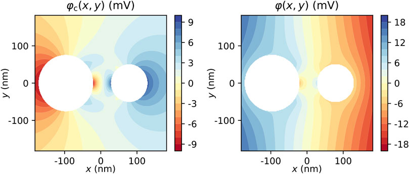
FIGURE 4. Cylinder potential (left) and total potential (right) for an external electric field of
The force follows from the integration of the surface charge density and electric field E = −grad φ over the surface S of the cylinder. The force component in a specific direction (arbitrary unit vector
For the force in x-direction,
For
Exploiting the orthogonality of the cosines, the force in x-direction then results in
with L being the length of the cylinder and Fc an abbreviation for the sum. The orthogonality of the trigonometric functions also yields Fy = 0.
In order to study the dependence of the force on distance and radii, we assume equal radii
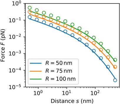
FIGURE 5. Analytical (solid lines) and numerical forces (circles) on a cylinder of length
The main reason for the discrepancies is that the analytical model does not consider the finite size effects and the top and bottom faces of the cylinders. The force decreases with the distance in the same way as for the two spheres. The transition between the corresponding two rates is again at roughly
Furthermore, it is interesting to investigate the force for the different cylinder radii
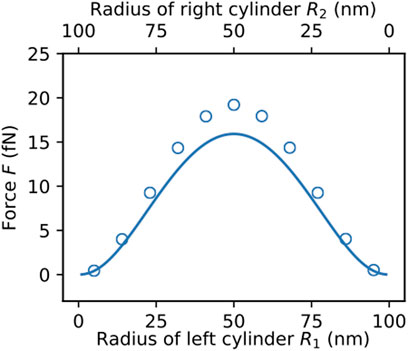
FIGURE 6. Analytical (solid lines) and numerical forces (circles) on a cylinder of length
The actual deflection
For the force as a point load on the tip, the stiffness can be written as
with the geometrical moment of intertia
For nanopillars with w = 100 nm and l = 1 µm, the stiffness therefore is kp(Si) N/m if it is made of Si (
For the force as a uniformly distributed load, the stiffness
is larger than for the point load. E.g., for a Si pillar with the same parameters as above, Kd = 1.5 kN/m. A combined expression for both cases can be written as
An expression for the deflection can be obtained by inserting the force Eq. 25. It reads
Since in both cases, a force at the tip or a length-distributed force, the stiffness depends on R4 and the force is proportional to a2, which for s < R roughly corresponds to R2, the deflection is approximately proportional to
For a width of w = 100 nm, a distance of d = 50 nm and an applied electric field of E0 = 1
It is important to notice that the presented modeling approach by means of two infinitely extended cylinders is only valid as long as the neutral axes of the two considered pillars remain nearly straight and parallel to each other. This involves two subconditions: First, the maximum deflection of the individual pillars imposed by electrostatic forces must be small so that the deviations of the real electrostatic induction and the associated charge distribution remain negligible in comparison to the our simplified model. Secondly, there must be no pull-in effect between the two adjacent pillars, i.e., the restoring elastomechanical force of the individual cantilever-like pillars must always be larger than the attractive electrostatic force between the pillars (Wen-Hui and Ya-Pu, 2003; Wang et al., 2004; Zhang and pu Zhao, 2006).
If both conditions are met, then the analytical model offers the great advantage that its evaluation with common mathematical toolboxes such as Wolfram Mathematica or direct implementations in, e.g., Python provides a good estimate of the occurring electrostatic excess field strengths, the electrostatic forces, and the fundamental system behavior within fractions of a second. In contrast, a solely computational analysis with COMSOL takes several minutes yielding comparable results. In the case of a parametric sweep as, e.g., depicted in Figure 5, this may even take several hours our days.
However, as soon as the modeling prerequisites are substantially violated, our strongly, simplified two-dimensional model loses its validity and must be replaced by a three-dimensional model of dielectric cantilevers exposed to a homogenous external electric field. The rigorous mathematical description of the electromechanical interaction between the two elastic pillars and the external electric field would be usefully implemented via the energy-momentum tensor of the dielectric material composed of two components (Penfield and Haus, 1967). The first component describes the elastomechanical properties of the cantilever-like pillar while the second component incorporates the electric field interaction. Mechanical and electrical components governing the electro-elastomechanical interaction are related to each other via a suitably selected material law. From this model, the electric field distribution in the field space would have to be calculated. As soon as this is known, the resulting force of electric origin on the pillar can be derived by simple integration over a closed surface, which encloses the pillar and runs completely in free space (Penfield and Haus, 1967).
As one can see, the exact theoretical description of this problem is quite complex and very likely does not have a closed-form analytical solution. Fortunately, the two conditions mentioned above were generally fulfilled in our considerations, so that our simplified two-dimensional model can be applied for the pillars discussed above. This can be seen in the example above, which estimated dynamical deflections up to 1 nm for a pillar diameter of 100 nm and a distance of 50 nm. Nevertheless, care must be taken for larger relative deflections.
One remaining question is how far the electric field strength can be increased, if the two aforementioned conditions of small deflections and large restoring force stay fulfilled. The limit faced here seems to be the maximum total field (
with e the electron charge, h the Planck constant, We the work function, m* the effective mass in the metal and m the electron mass in vacuum.
The mass ratio depends on many circumstances and is not isotropic. For Au, a value can be extracted from tables such as given in (Ashcroft and Mermin, 1976), where
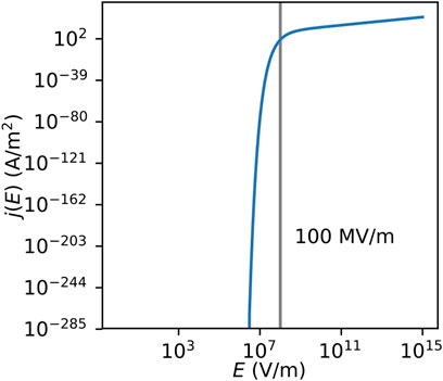
FIGURE 7. Field emission current density vs. applied electric field strength.
The total electric field between the nanopillars is larger than E0. The enhancement factor
A possibility to provide the electric field would be to implement coplanar electrodes on the substrate. The nanopillars would then be located between these electrodes. Depending on the size of the area reserved for the nanopillars, a distance del between these electrodes has to be chosen. This distance, in turn, determines the voltage
In this paper, analytical and numerical calculations for the electrostatics of two cylinders in an electric field have been used to study the possible electrostatic actuation of nanopillar dimers. While the associated electrostatic forces are very tiny, the pillars can be driven quasistatically to a deflection of up to
Detection or exploiting the effects of these small deflections remains a challenging task. The limit of detection of optical methods, which are the most accurate at the moment, are already capable of detecting, e.g., nanowire motion. Moreover, they are becoming ever more effective with new promising techniques emerging such as optical plasmonic transduction.
It should also be noted that the treatment in this paper was strictly electrostatic. With rising frequencies, there can be expected an increasing magnetic contribution, which was neglected in this manuscript. A comparison of the forces with the ones obtained in an electrodynamical approach and with optical forces should be performed in a future work.
Since there are several quantities having an influence on the electrostatic force and the stiffness of the pillars, it is possible to tweak the system in order to obtain even larger deflections, both statically and dynamically. In addition to geometrical dimensions these are, e.g., the materials involved, the arrangement of (arrays of) dimers and even using other systems than pillars. The approach may also be applied to pairs of nanostrings or nanowires. Especially due to their length, they can be driven presumably more effectively than the pillar dimers.
The original contributions presented in the study are included in the article/Supplementary Material, further inquiries can be directed to the corresponding author.
AK conceived the presented idea. AK and RB developed the theory and performed the computations. All authors discussed the results and contributed to the final manuscript.
This work is supported by the European Research Council under the European Union Horizon 2020 research and innovation program (Grant Agreement-716087-PLASMECS) and the Austrian Research Promotion Agency (FFG) under grant “H-iSlice” (number 869181). The Department of Integrated Sensor Systems gratefully acknowledges partial financial support by the European Regional Development Fund (ERDF) and the province of Lower Austria.
The authors declare that the research was conducted in the absence of any commercial or financial relationships that could be construed as a potential conflict of interest.
Bagci, T., Simonsen, A., Schmid, S., Villanueva, L. G., Zeuthen, E., Appel, J., et al. (2014). Optical detection of radio waves through a nanomechanical transducer. Nature 507, 81–85. doi:10.1038/nature13029
Chaste, J., Eichler, A., Moser, J., Ceballos, G., Rurali, R., and Bachtold, A. (2012). A nanomechanical mass sensor with yoctogram resolution. Nat. Nanotechnol. 7, 301–304. doi:10.1038/nnano.2012.42
Chien, M. H., Steurer, J., Sadeghi, P., Cazier, N., and Schmid, S. (2020). Nanoelectromechanical position-sensitive detector with picometer resolution. ACS Photonics. 7, 2197–2203. doi:10.1021/acsphotonics.0c00701
Cleland, A. N., and Roukes, M. L. (1996). Fabrication of high frequency nanometer scale mechanical resonators from bulk Si crystals. Appl. Phys. Lett. 69, 2653. doi:10.1063/1.117548
Davis, M. H. (1964). Two charged spherical conductors in a uniform electric field: forces and field strength. Q. J. Mech. Appl. Math. 17, 499–511. doi:10.1093/qjmam/17.4.499
Dohn, S., Schmid, S., Amiot, F., and Boisen, A. (2010). Position and mass determination of multiple particles using cantilever based mass sensors. Appl. Phys. Lett. 97, 044103. doi:10.1063/1.3473761
Emets, Y. P., and Onofrichuk, Y. P. (1996). Interaction forces of dielectric cylinders in electric fields. IEEE Trans. Dielectr. Electr. Insul. 3, 87–98. doi:10.1109/94.485519
Faust, T., Krenn, P., Manus, S., Kotthaus, J. P., and Weig, E. M. (2012). Microwave cavity-enhanced transduction for plug and play nanomechanics at room temperature. Nat. Commun. 3, 728–736. doi:10.1038/ncomms1723
Fowler, R. H., and Nordheim, L. (1928). Electron emission in intense electric fields. Proc. R. Soc. Lond. - Ser. A Contain. Pap. a Math. Phys. Character 119, 173–181. doi:10.1142/9789814503464˙0087
Hanay, M. S., Kelber, S., Naik, A. K., Chi, D., Hentz, S., Bullard, E. C., et al. (2012). Single-protein nanomechanical mass spectrometry in real time. Nat. Nanotechnol. 7, 602–608. doi:10.1038/nnano.2012.119
Jenss, H. (1932). Das potential isolierter sonden im homogenen felde. Archiv f. Elektrotechnik 26, 557–561. doi:10.1007/bf01660775
Kabashin, A., Evans, P., Pastkovsky, S., Hendren, W., Wurtz, G., Atkinson, R., et al. (2009). Plasmonic nanorod metamaterials for biosensing. Nat. Mater. 8, 867–871. doi:10.1038/nmat2546
Kainz, A., Keplinger, F., Hortschitz, W., Kahr, M., Steiner, H., Stifter, M., et al. (2019). Noninvasive 3d field mapping of complex static electric fields. Phys. Rev. Lett. 122, 244801. doi:10.1103/PhysRevLett.122.244801
Kainz, A., Steiner, H., Schalko, J., Jachimowicz, A., Kohl, F., Stifter, M., et al. (2018). Distortion-free measurement of electric field strength with a mems sensor. Nat Electron 1, 68–73. doi:10.1038/s41928-017-0009-5
Li, M., Tang, H. X., and Roukes, M. L. (2007). Ultra-sensitive nems-based cantilevers for sensing, scanned probe and very high-frequency applications. Nat. Nanotechnol. 2, 114–120. doi:10.1038/nnano.2006.208
Molina, J., Ramos, D., Gil-Santos, E., Escobar, J. E., Ruz, J. J., Tamayo, J., et al. (2020). Optical transduction for vertical nanowire resonators. Nano Lett. 20, 2359–2369. doi:10.1021/acs.nanolett.9b04909
Naik, A. K., Hanay, M. S., Hiebert, W. K., Feng, X. L., and Roukes, M. L. (2009). Towards single-molecule nanomechanical mass spectrometry. Nat. Nanotechnol. 4, 445–450. doi:10.1038/nnano.2009.152
Penfield, P., and Haus, H. A. (1967). Electrodynamics of moving media. Cambridge, England: MIT Press. doi:10.1063/1.3034557
Sadeghi, P., Wu, K., Rindzevicius, T., Boisen, A., and Schmid, S. (2017). Fabrication and characterization of au dimer antennas on glass pillars with enhanced plasmonic response. Nanophotonics 7, 497–505. doi:10.1515/nanoph-2017-0011
Sage, E., Brenac, A., Alava, T., Morel, R., Dupré, C., Hanay, M. S., et al. (2015). Neutral particle mass spectrometry with nanomechanical systems. Nat. Commun. 6, 6482–6485. doi:10.1038/ncomms7482
Schmid, S., Dohn, S., and Boisen, A. (2010). Real-time particle mass spectrometry based on resonant micro strings. Sensors 10, 8092–8100. doi:10.3390/s100908092
Schmid, S., Kurek, M., Adolphsen, J. Q., and Boisen, A. (2013). Real-time single airborne nanoparticle detection with nanomechanical resonant filter-fiber. Sci. Rep. 3, 1288. doi:10.1038/srep01288
Schmid, S., Bagci, T., Zeuthen, E., Taylor, J. M., Herring, P. K., Cassidy, M. C., et al. (2014). Single-layer graphene on silicon nitride micromembrane resonators. J. Appl. Phys. 115, 054513. doi:10.1063/1.4862296
Schmid, S., Villanueva, L. G., and Roukes, M. L. (2016). Fundamentals of nanomechanical resonators. 1st Edn. New York, NY: Springer International Publishing.
Schmid, S., Wendlandt, M., Junker, D., and Hierold, C. (2006). Nonconductive polymer microresonators actuated by the kelvin polarization force. Appl. Phys. Lett. 89, 163506. doi:10.1063/1.2362590
Thijssen, R., Kippenberg, T. J., Polman, A., and Verhagen, E. (2015). Plasmomechanical resonators based on dimer nanoantennas. Nano Lett. 15, 3971–3976. doi:10.1021/acs.nanolett.5b00858
Unterreithmeier, Q. P., Weig, E. M., and Kotthaus, J. P. (2009). Universal transduction scheme for nanomechanical systems based on dielectric forces. Nature 458, 1001–1004. doi:10.1038/nature07932
Villanueva, L. G., Karabalin, R. B., Matheny, M. H., Kenig, E., Cross, M. C., and Roukes, M. L. (2011). A nanoscale parametric feedback oscillator. Nano Lett. 11, 5054–5059. doi:10.1021/nl2031162
Wang, G.-W., Zhang, Y., Zhao, Y.-P., and Yang, G.-T. (2004). Pull-in instability study of carbon nanotube tweezers under the influence of van der waals forces. J. Micromech. Microeng. 14, 1119–1125. doi:10.1088/0960-1317/14/8/001
Wen-Hui, L., and Ya-Pu, Z. (2003). Dynamic behaviour of nanoscale electrostatic actuators. Chin. Phys. Lett. 20, 2070–2073. doi:10.1088/0256-307x/20/11/049
Yu, P. L., Purdy, T., and Regal, C. A. (2012). Control of material damping in high-Q membrane microresonators. Phys. Rev. Lett. 108, 083603, doi:10.1103/PhysRevLett.108.083603
Keywords: nanoelectromechanical systems, nanopillars, electrostatics, nanomechanical system, transduction, nanorods
Citation: Kainz A, Beigelbeck R and Schmid S (2021) Modeling the Electrostatic Actuation of Nanomechanical Pillar Dimers. Front. Mech. Eng 6:611590. doi: 10.3389/fmech.2020.611590
Received: 29 September 2020; Accepted: 31 December 2020;
Published: 19 February 2021.
Edited by:
Philip Feng, University of Florida, United StatesReviewed by:
Fan Ye, University of Massachusetts Amherst, United StatesCopyright © 2021 Kainz, Beigelbeck and Schmid. This is an open-access article distributed under the terms of the Creative Commons Attribution License (CC BY). The use, distribution or reproduction in other forums is permitted, provided the original author(s) and the copyright owner(s) are credited and that the original publication in this journal is cited, in accordance with accepted academic practice. No use, distribution or reproduction is permitted which does not comply with these terms.
*Correspondence: Andreas Kainz, YW5kcmVhcy5rYWluekBkb25hdS11bmkuYWMuYXQ=
Disclaimer: All claims expressed in this article are solely those of the authors and do not necessarily represent those of their affiliated organizations, or those of the publisher, the editors and the reviewers. Any product that may be evaluated in this article or claim that may be made by its manufacturer is not guaranteed or endorsed by the publisher.
Research integrity at Frontiers
Learn more about the work of our research integrity team to safeguard the quality of each article we publish.