 Kalle Kalliorinne
 Roland Larsson1
 Andreas Almqvist
- 1Division of Machine Elements, Luleå University of Technology, Luleå, Sweden
- 2Embedded Intelligent Systems, Luleå University of Technology, Luleå, Sweden
Predicting the contact mechanical response for various types of surfaces is and has long been a subject, where many researchers have made valuable contributions. This is because the surface topography has a tremendous impact on the tribological performance of many applications. The contact mechanics problem can be solved in many ways, with less accurate but fast asperity-based models on one end to highly accurate but not as fast rigorous numerical methods on the other. A mathematical model as fast as an asperity-based, yet as accurate as a rigorous numerical method is, of course, preferred. Artificial neural network (ANN)–based models are fast and can be trained to interpret how in- and output of processes are correlated. Herein, 1,536 surface topographies are generated with different properties, corresponding to three height probability density and two power spectrum functions, for which, the areal roughness parameters are calculated. A numerical contact mechanics approach was employed to obtain the response for each of the 1,536 surface topographies, and this was done using four different values of the hardness per surface and for a range of loads. From the results, 14 in situ areal roughness parameters and six contact mechanical parameters were calculated. The load, the hardness, and the areal roughness parameters for the original surfaces were assembled as input to a training set, and the in situ areal roughness parameters and the contact mechanical parameters were used as output. A suitable architecture for the ANN was developed and the training set was used to optimize its parameters. The prediction accuracy of the ANN was validated on a test set containing specimens not seen during training. The result is a quickly executing ANN, that given a surface topography represented by areal roughness parameters, can predict the contact mechanical response with reasonable accuracy. The most important contact mechanical parameters, that is, the real area of contact, the average interfacial separation, and the contact stiffness can in fact be predicted with high accuracy. As the model is only trained on six different combinations of height probability density and power spectrum functions, one can say that an output should only be trusted if the input surface can be represented with one of these.
1 Introduction
Surface topography plays an extremely important role in processes such as wear, friction, lubrication, sealing, contact resistance, and heat conduction. This is due to that the roughness causes local contacts between the surfaces, as in mixed lubrication, thus governing how the surface deforms and behaves in contact and defining the boundary friction and the real area of contact. The surface topography may be characterized by a number of areal roughness parameters defined in ISO 25178, see ISO Central Secretary (2012). These parameters have, however, limited correlation to the real area of contact, as well as to friction and wear processes, especially if only a few out of the complete set of field parameters are considered.
By using computational contact mechanics, we can estimate the real area of contact for a surface with given topography and also show how the areal roughness parameters change inside the contact. Notice that, an accurate and reliable result requires a highly resolved surface topography measurement. Thereby, the mesh considered in the numerical solution procedure will have to be of equal resolution, which, in turn, increases the computational time significantly. From an engineering point of view, a non-iterative model that swiftly yields relatively exact predictions of contact mechanics parameters, such as the real area of contact, would therefore be highly desired.
The Greenwood and Williamson (GW) theory (Greenwood and Williamson, 1966; Greenwood and Tripp, 1970) has been and still is very frequently used. Note that it was Archard (1957) who laid the foundation for most of the (multi)asperity-based type of models known of today (Nayak, 1971; Onions and Archard, 1973; Bush et al., 1975; Bush et al., 1979; Carbone, 2009; Greenwood et al., 2011). The Persson contact mechanics theory (Persson, 2006; Yang and Persson, 2008) is also a frequently used tool. Although being highly useful models that provide insight and yield rapid predictions, they are based on assumptions, making them not always very accurate. The GW theory assumes that the asperities at the surfaces exhibit Gaussian probability distributions. The asperities are also assumed to deform independently of each other which leads to that GW theory is applicable only when the contact area is small (compared with the nominal contact area). Persson’s theory assumes that the surfaces exhibit Gaussian height probability distributions and it considers interasperity coupling. Although Persson’s theory might not be very accurate for small real area of contact, it applies well to study the complete contact (see e.g. (Almqvist et al., 2011)). The study by Müser et al. (2017) summarizes findings obtained with various kinds of models, including asperity-based ones and Persson’s theory. Moreover, results from numerical brute force methods, all-atoms–based models, and experiments were presented as well. It was concluded that 1) rigorous numerical brute force approaches yield almost identical results on all properties, 2) Persson’s theory, all-atom simulations, and experiments could be used to identify the correct trends, and almost exact numbers for some properties, and 3) asperity models predicted the real area of contact rather well and provided alternative interpretations for other properties. It would be very useful if it was possible to obtain a mathematical model for fast calculation, which is as accurate as the rigorous models are, when predicting contact mechanics parameters such as real area of contact.
The ideal situation would be to describe surface topography by its height probability distribution and its power spectrum, which constitute the complete description. However, this complicates the analysis, and if a subset of the areal roughness parameters ISO Central Secretary (2012) would be sufficient, it would facilitate the analysis tremendously. In this study, we will present an artificial neural network (ANN)–based model. This model acts as a transfer function, taking areal roughness parameters as input and predicts the real area of contact and other contact mechanics parameters. A similar ANN-based approach has been used in contact mechanics before (see (Rapetto et al., 2009)). Other examples where ANN-based approaches have been used in tribology are Nasir et al. (2010), Nirmal (2010), Ćirović et al. (2012), and Moder et al. (2018). If an ANN, which executes much faster than a computational contact mechanics approach, is well designed, trained, and tested, it can thus provide reasonably accurate predictions of tribological performance parameters very rapidly.
The idea with the present work is to generate thousands of surfaces by means of the method developed by Pérez-Ràfols and Almqvist (2019), and to compute parameters, such as the real area of contact and areal roughness parameters when these surfaces are pressed into contact with a flat rigid counter surface. To this end, we will use the computational contact mechanics approach presented by Almqvist et al.( 2007), which was further developed by Sahlin et al. (2010).
The ANN is trained to find the relationship between the surfaces’ original, the in-contact, that is, in situ areal roughness parameters and the contact mechanics parameters, for a range of loads, spanning from no load at all to a load that causes nearly as much as 50% real area of contact.
2 Methods
This section presents, in a workflow order, the implementation of the ANN. It starts with describing surface topography generation, followed by preprocessing and a brief description of the contact mechanics approach adopted, and it ends with a presentation of the architecture of artificial neural network that was developed herein.
2.1 Surface Topography Generation
Training neural networks requires large data sets. Therefore, it is necessary to generate a wide range of different surface topographies. The surface randomization algorithm developed by Pérez-Ràfols and Almqvist (2019) was employed to randomly generate 2,022 surfaces topographies with given height probability distribution (HPD) and a power spectrum (PS). The HPD and PS can be mathematically modeled by classical distribution and spectrum functions, but they may also be obtained (and adapted) from measured surface topographies. In this work, mathematical models for Gaussian, bi-Gaussian and Weibull functions, and self-affine and exponential PS functions were used. The reader is referred to Pérez-Ràfols and Almqvist (2019) for a precise description of these HPD and PS. A surface topography generation selection scheme is depicted in Figure 1, where one type of HPD and PS is selected together with the corresponding shape-defining parameters, that is, c, k, H, β, α, q0, and q1. Remark that the HPDs are defined with zero mean value and unit standard deviation. With these constrains, the Gaussian HPD requires no input, while the bi-Gaussian and the Weibull distributions may be defined using one parameter, that is, c and k, respectively. Specifying the PS requires four parameters, that is, the Hurst exponent H for the self-affine and the parameter β, which defines the autocorrelation length
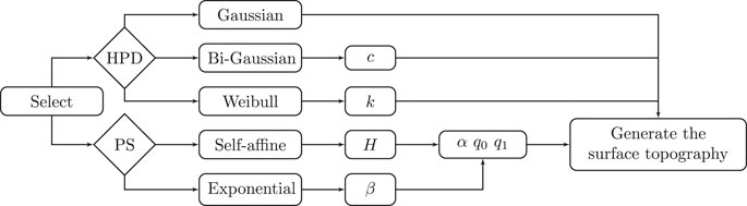
FIGURE 1. Surface topography generation scheme.
Figure 2 shows an example of a generated surface, using the bi-Gaussian HPD model and the self-affine PS model. The corresponding parameter settings are displayed to the right.
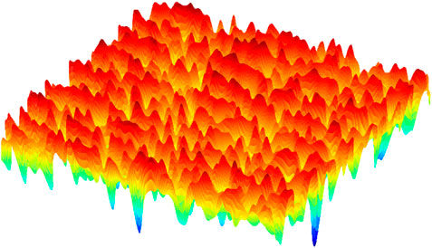
FIGURE 2. A randomized surface, generated by following the scheme in Figure 1, using the settings presented to the right.
The parameter space for the surface dataset used for training was defined by four equidistantly spaced values for each of the seven parameters (
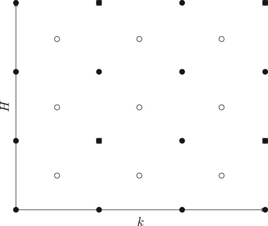
FIGURE 3. The parameter space for the
2.2 Preprocessing and Contact Mechanics
The areal roughness parameters in Table 1 are calculated for all of the 2,022 surfaces, which are made dimensionless by scaling to exhibit unit rms roughness, that is,
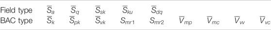
TABLE 1. Areal roughness parameters calculated according to ISO Central Secretary (2012).
The dimensionless areal roughness parameters (for the scaled surfaces) in Table 1 are calculated according to ISO Central Secretary (2012). They are grouped as parameters of field type and of Bearing Area Curve (BAC) type. These parameters are the input for the ANN described in Section 2.3, with architecture illustrated in Figure 4. For more details on how to calculate the areal roughness parameters according to the standard, see Blateyron (2013). As a result of the contact mechanics simulations, the surfaces may be plastically deformed, and it is the hardness
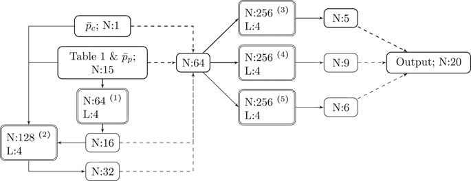
FIGURE 4. Multitask neural network architecture, with
The output from the contact mechanics calculations are the in situ, areal roughness parameters, and the six contact mechanics parameters in Table 2. These are the real area of contact to nominal contact area ratio

TABLE 2. Contact mechanics parameters.
2.3 The Artificial Neural Network
Here, the ANN architecture depicted in Figure 4, which is engineered to predict the contact mechanical response of surfaces represented by the areal roughness parameters (given in Table 1), will be described. The areal roughness parameters in Table 1 and the dimensionless hardness
The first subnetwork(1), with 64 neurons, has rectifier (ReLU) activation functions
The input to the first and second subnetworks and their output are assembled into one vector with 64 values. This vector is the input to each of the three parallel subnetworks(3)–(5), which have softplus (smooth rectifying) activation functions
3 Results and Discussion
First, in Section 3.1, the performance of the ANN model will be evaluated with linear regression between predicted values and the output in the test dataset. Then, in Section 3.2, examples of how the predictions changes with the load will be presented and compared to the correct values.
3.1 Predicting Contact Mechanical Response
Herein, the test set, which contains 1,458 specimens that it has never seen before, is used to evaluate the ANN’s predictive performance on surfaces for a whole range of loads. Depicted in Figures 5, 6 are linear regression of all the predicted parameter values and the
where y is the target output,
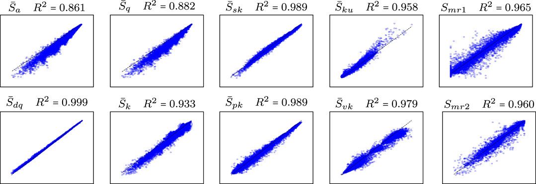
FIGURE 5. Linear regression of target (x-axis) and predicted (y-axis) outputs.
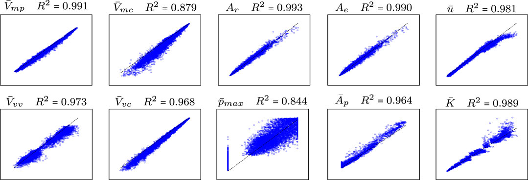
FIGURE 6. Linear regression of target (x-axis) and predicted (y-axis) outputs.
There is much that can be said about the results presented in Figure 6. One thing, which is nearly impossible not to notice, is the regression for the dimensionless maximum pressure
3.2 Application
In this section, the accuracy of the predictions of the ANN for three different test specimens, taken from the test set that the network never has seen before, will be investigated over the whole range of loads considered when the test set was generated with the contact mechanics simulations. The test specimens are listed in Tables 3, 4, and they consist of the areal roughness parameters, corresponding to the surfaces topographies presented in Figure 7, combined with a value of the dimensionless hardness.
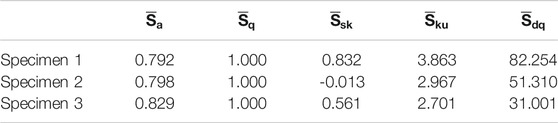
TABLE 3. Test specimens containing the dimensionless areal roughness parameters, corresponding to the topographies depicted in Figure 7 and a value of the dimensionless hardness: part 1—field type parameters.
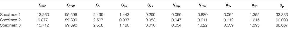
TABLE 4. Test specimens containing the dimensionless areal roughness parameters, corresponding to the topographies depicted in Figure 7 and a value of the dimensionless hardness: part 2—BAC type parameters and dimensionless hardness.
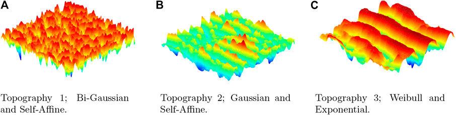
FIGURE 7. Surface topographies for the three test specimens (A–C) with dimensionless areal roughness paraeters and hardness, listed in Tables 3, 4.
The predictions of the in situ dimensionless mean square height
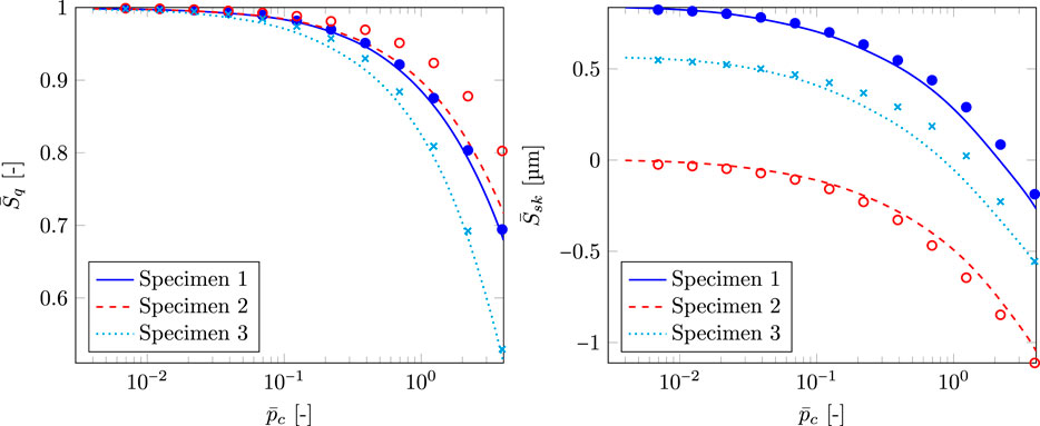
FIGURE 8. Dimensionless root mean square height
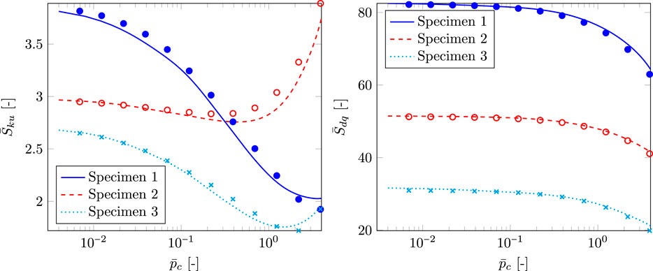
FIGURE 9. Dimensionless kurtosis
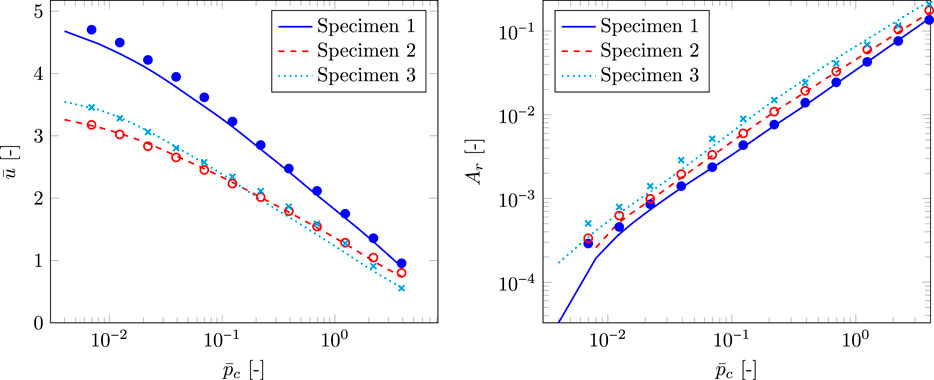
FIGURE 10. Dimensionless average interfacial separation
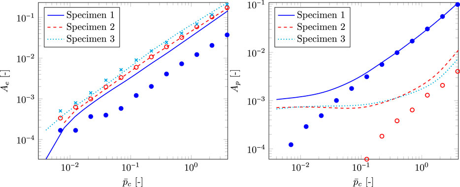
FIGURE 11. Real area of elastic contact ratio
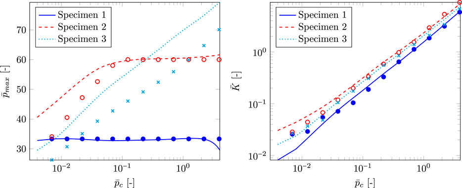
FIGURE 12. Dimensionless maximum pressure
The predictions of the in situ dimensionless kurtosis
The predictions of the dimensionless average interfacial separation
The predictions of the elastic part of the real area of contact ratio
The predictions of the dimensionless maximum pressure
4 Concluding Remarks
Two datasets containing a total of 2,022 different surface topographies were generated using the algorithm developed by Pérez-Ràfols and Almqvist (2019). Three different HPD functions and two different PS functions were obtained from Gaussian, bi-Gaussian, and Weibull HPD functions and self-affine and exponential PS functions, described with as few shape-defining parameters as possible. Fourteen areal roughness parameters were calculated for all surfaces in the dataset. Together with the surface indentation hardness and a given applied load, these 14 areal roughness parameters were used as input for the ANN.
A numerical elastoplastic contact mechanics approach, in which the hardness limits the maximum pressure the surface can exhibit before it yields plastically, was then employed to perform simulations of pressing each of the generated surfaces against a flat rigid counter surface for a sequence of loads. Since four values for the hardness were considered for the training set with 1,536 different surface topographies and three were considered for the test set with 486 topographies, a grand total of
An architecture for an artificial neural network (ANN), which consisted of five different subnetworks, was designed and trained on the dataset. Linear regression was applied, and the
Summing up, the ANN can be used to roughly appreciate the in situ behavior of various kinds of surface topographies, if the areal roughness parameters, the indentation hardness, and the nominal contact pressure are known. Some parameters, that is, the real area of contact ratio, the dimensionless average interfacial separation, and contact stiffness can actually be predicted with high accuracy.
Data Availability Statement
The raw data supporting the conclusion of this article will be made available by the authors, without undue reservation.
Author Contributions
KK has performed the main part of the development of the ANN-based model and has been coordinating the writing. RL contributed with expertise, to the discussions and was engaged in the writing. FR has been engaged in surface generation and contact mechanics and contributed to the writing. ML contributed with expertise, particularly regarding AI and machine learning, contributed to discussions and to the writing. AA has initiated the work and has been involved in all parts of it.
Conflict of Interest
The authors declare that the research was conducted in the absence of any commercial or financial relationships that could be construed as a potential conflict of interest.
Acknowledgments
The authors would like to acknowledge the support from VR (The Swedish Reseach Council): DNR 2019-04293.
Nomenclature
References
Almqvist, A., and Pérez-Ràfols, F. (2019). Scientific Computing with Applications in Tribology: A Course Compendium. Luleå, Sweden: Luleå University of Technology
Almqvist, A., Campañá, C., Prodanov, N., and Persson, B. N. J. (2011). Interfacial Separation between Elastic Solids with Randomly Rough Surfaces: Comparison between Theory and Numerical Techniques. J. Mech. Phys. Sol. 59 (11), 2355–2369. doi:10.1016/j.jmps.2011.08.004
Almqvist, A., Sahlin, F., Larsson, R., and Glavatskih, S. (2007). On the Dry Elasto-Plastic Contact of Nominally Flat Surfaces. Tribology Int. 40 (4), 574–579. doi:10.1016/j.triboint.2005.11.008
Archard, J. F. (1957). Elastic Deformation and the Laws of Friction. Proc. R. Soc. Lond. A 243 (1233):190–205. doi:10.1098/rspa.1957.0214
Blateyron, F. (2013). The Areal Field Parameters. Berlin, Heidelberg: Springer Berlin Heidelberg, 15–43. doi:10.1007/978-3-642-36458-7_2
Bush, A. W., Gibson, R. D., and Keogh, G. P. (1979). Strongly Anisotropic Rough Surfaces. Trans. ASME. J. Lubrication Tech. 101 (1), 15–20. doi:10.1115/1.3453271
Bush, A. W., Gibson, R. D., and Thomas, T. R. (1975). The Elastic Contact of a Rough Surface. Wear 35 (1), 87–111. doi:10.1016/0043-1648(75)90145-3
Ćirović, V., Aleksendrić, D., and Mladenović, D. (2012). Braking Torque Control Using Recurrent Neural Networks. Proc. Inst. Mech. Eng. D: J. Automobile Eng. 226 (6), 754–766. doi:10.1177/0954407011428720
Carbone, G. (2009). A Slightly Corrected Greenwood and Williamson Model Predicts Asymptotic Linearity between Contact Area and Load. J. Mech. Phys. Sol., 57(7):1093–1102. doi:10.1016/j.jmps.2009.03.004
ISO Central Secretary (2012). Geometrical Product Specifications (Gps)—Surface Texture: Areal—Part 2: Terms, Definitions and Surface Texture Parameters. Geneva, CH: International Organization for StandardizationAvailable at: https://www.iso.org/standard/42785.html
Greenwood, J. A., Putignano, C., and Ciavarella, M. (2011). A Greenwood & Williamson Theory for Line Contact. Wear 270, 332–334. doi:10.1016/j.wear.2010.11.002
Greenwood, J., and Tripp, J. (1970). The Contact of Two Nominally Flat Rough Surfaces. Proc. Inst. Mech. Eng. 185, 625–634. doi:10.1243/pime_proc_1970_185_069_02
Greenwood, J., and Williamson, J. (1966). Contact of Nominally Flat Surfaces. Proc. R. Soc. Lond. A 295, 300–319. doi:10.1098/rspa.1966.0242
Müser, M. H., Dapp, W. B., Bugnicourt, R., Sainsot, P., Lesaffre, N., Lubrecht, A. A., et al. (2017). Meeting the Contact-Mechanics Challenge. Tribology Lett. 65 (4), 118. doi:10.1007/s11249-017-0900-2
Moder, J., Bergmann, P., and Grün, F. (2018). Lubrication Regime Classification of Hydrodynamic Journal Bearings by Machine Learning Using Torque Data. Lubricants 6 (4). 108. doi:10.3390/lubricants6040108
Nasir, T., Yousif, B. F., McWilliam, S., Salih, N. D., and Hui, L. T. (2010). An Artificial Neural Network for Prediction of the Friction Coefficient of Multi-Layer Polymeric Composites in Three Different Orientations. Proc. Inst. Mech. Eng. C: J. Mech. Eng. Sci. 224 (2), 419–429. doi:10.1243/09544062jmes1677
Nayak, P. R. (1971). Random Process Model of Rough Surfaces. J. Lubrication Tech. 93 (3), 398–407. doi:10.1115/1.3451608
Nirmal, U. (2010). Prediction of Friction Coefficient of Treated Betelnut Fibre Reinforced Polyester (T-bfrp) Composite Using Artificial Neural Networks. Tribology Int. 43 (8), 1417–1429. doi:10.1016/j.triboint.2010.01.013
Onions, R. A., and Archard, J. F. (1973). The Contact of Surfaces Having a Random Structure. J. Phys. D: Appl. Phys. 6 (3), 289–304. doi:10.1088/0022-3727/6/3/302
Persson, B. N. J. (2006). Contact Mechanics for Randomly Rough Surfaces. Surf. Sci. Rep. 61, 201–227. doi:10.1016/j.surfrep.2006.04.001
Pérez-Ràfols, F., and Almqvist, A. (2019). Generating Randomly Rough Surfaces with Given Height Probability Distribution and Power Spectrum. Tribology Int. 131, 591–604. doi:10.1016/j.triboint.2018.11.020
Pérez-Ràfols, F., Larsson, R., and Almqvist, A. (2016). Modelling of Leakage on Metal-To-Metal Seals. Tribology Int. 94, 421–427. doi:10.1016/j.triboint.2015.10.003
Pérez-Ràfols, F., Larsson, R., van Riet, E. J., and Almqvist, A. (2018). On the Loading and Unloading of Metal-To-Metal Seals: A Two-Scale Stochastic Approach. Proc. Inst. Mech. Eng. Part J: J. Eng. Tribology 232 (12), 1525–1537. doi:10.1177/1350650118755620
Rapetto, M. P., Almqvist, A., Larsson, R., and Lugt, P. M. (2009). On the Influence of Surface Roughness on Real Area of Contact in Normal, Dry, Friction Free, Rough Contact by Using a Neural Network. Wear 266 (5), 592–595. doi:10.1016/j.wear.2008.04.059
Sahlin, F., Larsson, R., Marklund, P., Lugt, P. M., and Almqvist, A. (2010). A Mixed Lubrication Model Incorporating Measured Surface Topography. Part 1: Theory of Flow Factors. Proc. Inst. Mech. Eng. Part J: J. Eng. Tribology 224 (4), 335–351. doi:10.1243/13506501jet658
Spencer, A., Almqvist, A., and Larsson, R. (2011). A Semi-deterministic Texture-Roughness Model of the Piston Ring-Cylinder Liner Contact. Proc. Inst. Mech. Eng. Part J: J. Eng. Tribology 225 (6), 325–333. doi:10.1177/1350650110396279
Spencer, A., Avan, E. Y., Almqvist, A., Dwyer-Joyce, R. S., and Larsson, R. (2013). An Experimental and Numerical Investigation of Frictional Losses and Film Thickness for Four Cylinder Liner Variants for a Heavy Duty Diesel Engine. Proc. Inst. Mech. Eng. Part J: J. Eng. Tribology 227 (12), 1319–1333. doi:10.1177/1350650113491244
Yang, C., and Persson, B. N. J. (2008). Contact Mechanics: Contact Area and Interfacial Separation from Small Contact to Full Contact. J. Phys. Condensed Matter 20, 1–13. doi:10.1088/0953-8984/20/21/215214
Keywords: artificial neural networks, contact mechanics, surface roughness, average interfacial separation, real area of contact
Citation: Kalliorinne K, Larsson R, Pérez-Ràfols F, Liwicki M and Almqvist A (2021) Artificial Neural Network Architecture for Prediction of Contact Mechanical Response. Front. Mech. Eng 6:579825. doi: 10.3389/fmech.2020.579825
Received: 03 July 2020; Accepted: 30 November 2020;
Published: 18 May 2021.
Edited by:
Marco Paggi, IMT School for Advanced Studies Lucca, ItalyReviewed by:
Li Chang, The University of Sydney, AustraliaValentin L. Popov, Technical University of Berlin, Germany
Copyright © 2021 Kalliorinne, Larsson, Pérez-Ràfols, Liwicki and Almqvist. This is an open-access article distributed under the terms of the Creative Commons Attribution License (CC BY). The use, distribution or reproduction in other forums is permitted, provided the original author(s) and the copyright owner(s) are credited and that the original publication in this journal is cited, in accordance with accepted academic practice. No use, distribution or reproduction is permitted which does not comply with these terms.
*Correspondence: Kalle Kalliorinne, a2FsbGUua2FsbGlvcmlubmVAbHR1LnNl