Comparative Analysis of Error Sources in the Determination of Wear Volumes of Oscillating Ball-on-Plane Tests

The accurate determination of wear volumes is a prerequisite for the study of numerous tribological phenomena. Wear volumes can be measured with different techniques (profilometry, confocal microscopy, white light interferometry, atomic force microscopy) or else be calculated starting from some quantities (usually the width and the planimetric wear) measured from the wear scar. Advantages and drawbacks of the mentioned measuring techniques are shown by means of wear scars and calottes resulting from ball-on-plane tests with 100Cr6 specimens. When measuring wear volumes, white light interferometry results to be one of the most suitable techniques, since it offers high accuracy and is not as time consuming as atomic force microscopy. When wear volumes are calculated, errors result mainly from two sources: (1) the arbitrary choice of one or few line profiles for the determination of the width and of the planimetric wear, and (2) approximations in the calculation, which are even necessary when values of the wear volumes of the single tribological partners, i.e., ball and plane, and not only the total volume, are of interest. The effect of both the statistical distribution of values of the width and of the planimetric wear and the propagation of errors due to approximations on the accuracy in the determination of wear volumes is characterized and elucidated by examples. It is found that errors due to approximations are negligible when compared to errors due to the arbitrary choice of one line profile.

Introduction

The variation in volumetric wear data from tribological tests is quite large. Volumetric wear is a value influenced by the whole tribological system (Meng and Ludema, 1995) and its variation affects seriously the repeatability and reproducibility of tribological measurements and hence the determination of wear coefficients k. Many properties of the system are unknown and therefore not predictable. The variation of the material of the specimens due to production process, grinding, polishing or heat treatment, and properties of tribometers such as stiffness of the mechanical elements or the accuracy of sensors are only few examples of parameters influencing the volumetric wear, the wear coefficient and/or their determination. Through additional sources of error in the determination of the volumetric wear, the chance to identify error sources in the system and to recognize correlations with experimental parameters is further reduced (Reichelt and Cappella, 2020). Therefore, it is essential to determine and to minimize all possible sources of error in the method for the determination of the volumetric wear.

The methods for the determination of the volumetric wear have changed due to novel capabilities of microscopy tools and technologies. In the past, tactile devices were employed to measure individual lines perpendicular to the sliding direction, which in turn are used to calculate the wear volume. Rarely the entire friction track was recorded using many profile lines. Rather, the volume was calculated analytically from one or some of these lines. Today, white light interferometers (WLI), laser scanning systems, confocal microscopes, atomic force microscopes (AFM) etc. offer together with their analysis software a variety of possibilities to determine the wear volume more precisely within a reasonable measuring time.

Tactile profilometers (Yost, 1983; Wehbi et al., 1986; Kalin and Vizentin, 2000) for measuring roughness have been on the market since the 1930s. A diamond tip serves as a scanning probe. It is brought into contact with the surface and moved over the surface under contact forces that do not damage or even deform the sample. The contact force is kept constant by controlling the deflection of the tip. The electrical voltage required for the deflection of the tip is recorded and converted into the corresponding height profile. Distances of a few centimeters can be recorded with height differences of a few hundred micrometers. 3D measurements are extremely time-consuming due to the low scanning speed, so that usually just profile lines are recorded.

Non-contact optical measuring instruments, which have been available only since the 1980s and have been providing scientifically usable results since the 1990s through standardization, including calibration, are more suitable for fast surface measurements. White light interferometer microscopes (WLI) (Guilemany et al., 2001; Cox, 2006) are widely used in tribology. In these microscopes the interference of broadband white light is used to measure the topography of surfaces. The resolution of this optical method is better than that of profilometers (some hundreds of nanometers instead of 1 μm). However, at maximum resolution, the measuring field is limited to a few hundred micrometers. This increases the measuring time and requires stitching (the combination of multiple images to form an overall topography image), which is subject to errors. WLI is an indirect measurement of the height.

Atomic force microscopy (AFM) (Bhushan, 2001, 2003; Yu et al., 2009) is the method with the best resolution and the lowest susceptibility to errors, since it is a direct measurement of heights. A deflectable cantilever with a tip at its end serves as a scanning probe. The radius of the tip is usually in the range 5–20 nm. A laser beam is focused on the cantilever and the reflected beam changes its angle when the cantilever deflects. The deflection is thus detected by a four-quadrant photodiode. The position of the sample in the z-direction is controlled by means of piezos to ensure a constant deflection of the cantilever. The piezo voltage required for this purpose is converted to the corresponding height z. AFM has a sub-nanometer resolution, both laterally and vertically. The major disadvantage of this measuring method is the very small measuring range both laterally (some tens of microns) and in height (some microns). By time-consuming stitching these ranges can be theoretically many times larger. However, the gained accuracy does not justify in most cases the very long measuring time.

In the present article, the method for the calculation of volumetric wear in oscillating sliding tests with a ball-on-plane configuration is described and errors arising from approximations are analyzed. Furthermore, this method is exemplarily applied to a tribological test result without significant anomalies on the wear track and compared with WLI measurements. Also, the values of volumes determined through WLI is compared with AFM measurements. In this way, both errors due to measurement techniques and to calculation methods can be estimated.

Results

Calculation of Volumetric Wear

The total wear volume W_v is the sum of the wear volume of the ball, W_{v, ball}, and that of the plane, W_{v, flat}:

$\begin{array}{ll}{W}_v=W_{v,flat}+W_{v,ball}.& (1)\end{array}$

When the direct measurement of the volumes is not possible, they must be calculated using the ball radius R, the planimetric wear W_q, and the track width d_⊥, determined through profile measurements. This method (W_q method) is exposed in the following. The analysis of the procedure for the calculation of the wear volumes is important also for comparison of experiments in which volumes have partly been measured and partly calculated, as it is usually the case for old experiments.

In the middle of the wear track of the plane, a profile line perpendicular to the sliding direction is plotted, from which the track width d_⊥ and the planimetric wear W_q can be determined (Figure 1). Both d_⊥ and W_q depend strongly on the roughness of the unworn surface and on the roughness of the scar, which influence significantly the accuracy in the determination of the zero value of the height and hence the identification of scar borders. Errors resulting from this issue may vary considerably due to automated analysis or to individual discretion.

FIGURE 1

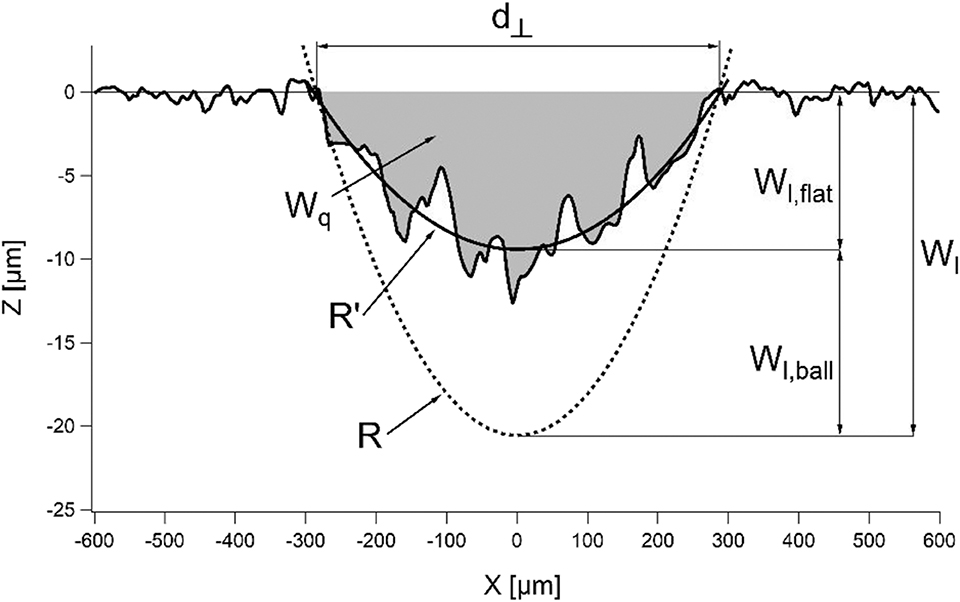
Figure 1. Line profile of a wear track on a 100Cr6 plane taken from a WLI measurement. The picture shows the track width d_⊥, the planimetric wear W_q (cross-sectional area of the wear track, filled in gray), the fitted circumference with radius of curvature R′, the circumference with known sphere radius R, the total linear wear W_l, and the linear wear of ball and plane, W_{l, ball} and W_{l, flat}.

In the following, Figure 2 is used to show how R′ of a wear scar is calculated.

FIGURE 2

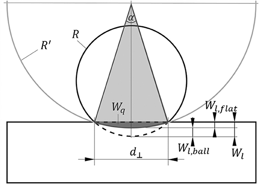
Figure 2. Schematic representation of the geometry of the worn sphere and plane normal to the sliding direction. The figure shows the quantities used to calculate the radius of the curved worn surface R′ in the friction test: radius of the ball R, wear track width d_⊥, angle of the circular sector α, planimetric wear W_q, total linear wear W_l, and linear wear of ball and plane, W_{l, ball} and W_{l, flat}. The original surface profile lines of the sphere and plane are shown as dashed lines.

From the geometry shown in Figure 2 follows:

$\begin{array}{ll}{W}_q={R^{\prime }}^{2}arcsin\left(\frac{d_{\perp }}{2R^{\prime }}\right)-\frac{1}{2}{R}^{\prime }{d}_{\perp }\sqrt{1-{\left(\frac{d_{\perp }}{2R^{\prime }}\right)}^2}.& (2)\end{array}$

If d_⊥ ≪ R′, the following approximations result from Taylor developments:

$\begin{array}{ll}arcsin\left(\frac{d_{\perp }}{2R^{\prime }}\right)\cong \frac{d_{\perp }}{2R^{\prime }}+\frac{1}{6}{\left(\frac{d_{\perp }}{2R^{\prime }}\right)}^3& (3)\end{array}$

and

$\begin{array}{ll}\sqrt{1-{\left(\frac{d_{\perp }}{2R^{\prime }}\right)}^2}\cong 1-\frac{1}{2}{\left(\frac{d_{\perp }}{2R^{\prime }}\right)}^2.& (4)\end{array}$

Substituting in Equation (2), we get:

$\begin{array}{ll}{W}_q\cong \frac{d_{\perp }^3}{12R^{\prime }}.& (5)\end{array}$

If the track width d_⊥ and the planimetric wear W_q are known, the radius R′ of the wear track can be calculated:

$\begin{array}{ll}R\prime \cong R_{app}\prime =\frac{d_{\perp }^3}{12W_q}& (6)\end{array}$

Hence, the wear volume of the plane is given by:

$\begin{array}{l}{W}_{v,flat}=\frac{1}{3}\pi W_{l,flat}^2\left(3R^{\prime }-W_{l,flat}\right)+W_q\Delta x\\ \cong \frac{{\pi d}_{\perp }^4}{64R^{\prime }}+W_q\Delta x,& (7)\end{array}$

where W_{l, flat} is the linear wear of the plane and Δx the stroke. Using the total linear wear W_l, the wear volume of the ball can be written as:

$\begin{array}{l}{W}_{v,ball}=\frac{1}{3}\pi {W_l}^2(3R{-W}_l)-\frac{1}{3}\pi W_{l,flat}^2(3R^{\prime }-W_{l,flat})\\ =\frac{1}{3}\pi {\left(\frac{d_{\perp }^2}{8R}\right)}^2\left(3R-\frac{d_{\perp }^2}{8R}\right)-\frac{1}{3}\pi {\left(\frac{d_{\perp }^2}{8R^{\prime }}\right)}^2\\ \left(3R^{\prime }-\frac{d_{\perp }^2}{8R^{\prime }}\right)\cong \pi \frac{d_{\perp }^4}{64}\left(\frac{1}{R}-\frac{1}{R^{\prime }}\right),& (8)\end{array}$

where the higher terms proportional to $d_{\perp }^6$ have been neglected both in Equations (7) and (8).

The total wear volume W_v can be calculated without approximations and is given by:

$\begin{array}{l}{W}_v=\pi R^3{\left(1-\sqrt{1-{\left(\frac{d_{\perp }}{2R}\right)}^2}\right)}^2\\ -\frac{1}{3}\pi R^3{\left(1-\sqrt{1-{\left(\frac{d_{\perp }}{2R}\right)}^2}\right)}^3+W_q\Delta x.& (9)\end{array}$

The approximation ${\left(1-\sqrt{1-{(\frac{d_{\perp }}{2R})}^2}\right)}^3\cong 0$ yields a slightly larger value of W_v:

$\begin{array}{ll}{W}_v\cong \pi R^3{\left(1-\sqrt{1-{\left(\frac{d_{\perp }}{2R}\right)}^2}\right)}^2+W_q\Delta x.& (10)\end{array}$

On the contrary, the approximation $\sqrt{1-{\left(\frac{d_{\perp }}{2R}\right)}^2}\cong 1-\frac{1}{2}{\left(\frac{d_{\perp }}{2R}\right)}^2$ reduces W_v:

$\begin{array}{ll}{W}_v\cong \frac{1}{4}\pi R^3{\left(\frac{d_{\perp }}{2R}\right)}^4\left(1-\frac{1}{6}{\left(\frac{d_{\perp }}{2R}\right)}^2\right)+W_q\Delta x.& (11)\end{array}$

Using both approximations, we get:

$\begin{array}{ll}{W}_v\cong \pi \frac{d_{\perp }^4}{64R}+W_q\Delta x.& (12)\end{array}$

In all cases in which the length of the calotte is different from its width (d_|| ≠ d_⊥), d_⊥ must be replaced by $\sqrt{d_{\left|\right|}{d}_{\perp }}$ [e.g., in Equations (7), (8), and (12)].

It is important to remember that the error in the determination of R′ does not affect the calculation of the total wear volume W_v [see Equation (9)]. Nevertheless, it affects indeed the calculation of the wear volumes of the single partners [see Equations (7) and (8)]. Therefore, it is important to analyze the error done through the approximations in Equations (3) and (4).

The error due to both approximations is shown in Figure 3 by comparing R′_app [Equation (6)] and the numerical solution of Equation (2) for R′. The approximation always leads to an underestimation of R′ (R′_app < R′).

FIGURE 3

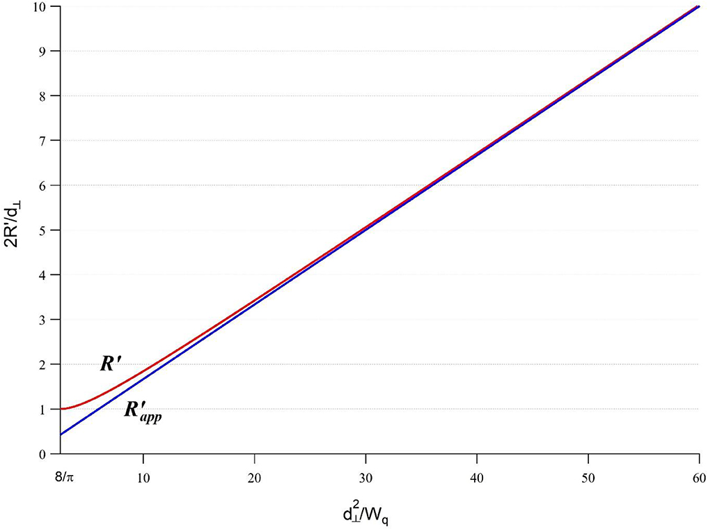
Figure 3. Comparison of the exact numerical solution of Equation (2) (upper curve, red) with the approximated solution (lower curve, blue) of the calculation of R′ from Equation (6). The diagram shows the ratio of twice the radius R′ to track width d_⊥ over the ratio of the square of the track width $d_{\perp }^2$ to the planimetric wear W_q.

The error of the approximation of R′ reaches a maximum when the ball does not wear and the plane wears maximally with R′ = R = W_l = d_⊥/2. The area W_q in this case is half the area of a circle with diameter d_⊥, $\pi d_{\perp }^2$/8, and the approximation in Equation (6) yields R′_app ≅ 2d_⊥/3π = 4R/3π = 0.424R. The maximum deviation (R′ − R′_app)/R′ in this extreme case amounts to 1–4/3π ≅ 57.6% and can also be seen in Figure 4, which shows the relative error of the approximate equation. One can see that the error is <10% if 2R′/d_⊥ > 1.8 (i.e., d_⊥ < 1.1R′); for 2R′/ d_⊥ > 2.485 (i.e., d_⊥ < 0.8R′) the error is even <5%.

FIGURE 4

Figure 4. Relative error in the calculation of R′ by using the approximation in Equation (6) over the ratio of twice the radius of curvature R′ to the track width d_⊥.

As concerns the propagation of the error on R′ in the functions expressing the volumes, it is easy to show that ∂W_{v, flat}(∂R′) = –∂W_{v, ball}(∂R′), since W_v does not depend on R′.

Further, by neglecting the terms proportional to $d_{\perp }^6$ as in Equations (7) and (8), we get:

$\begin{array}{ll}\frac{\partial \left(W_{v,flat}-W_q\Delta x\right)}{W_{v,flat}-W_q\Delta x}=\left(1-\frac{2}{\sqrt{1-{\left(\frac{d_{\perp }}{2R^{\prime }}\right)}^2}}\right)\frac{\partial R^{\prime }}{R^{\prime }}.& (13)\end{array}$

Hence, the error on W_{v, flat} due to the error on R′ is always negative and is between −∂R′/R′ and −2∂R′/R′ for 0 < d_⊥ < 1.5R′.

Comparison of AFM and WLI Measurements

In order to investigate the accuracy of the WLI images, comparative measurements were carried out after a tribological test by means of stitched AFM contact measurements on the surfaces of the 100Cr6 plane and the 100Cr6 sphere (R = 2 mm). WLI images were acquired with a NewView 5022 (Zygo, Middlefield, Connecticut). For AFM measurements, a Cipher (Asylum Research, Santa Barbara, California) was used with a maximum lateral scanning range of 30 μm and a vertical range of 3 μm. The AFM tip had a radius of ~15–20 nm.

The WLI image of the wear track of the plane is shown in Figure 5.

FIGURE 5

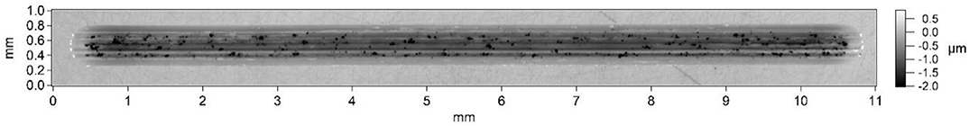
Figure 5. WLI image of a wear track on the plane.

A series of AFM topographies was acquired on the sphere and on the plane transverse to the sliding direction (26 and 28 images, respectively), and the images were then combined into two single images. These images, together with the profile lines extracted from them, are shown in Figure 6. They cover only a small part of the WLI images. Since the topography of the calotte perpendicular to the sliding direction is quite uniform, one line profile is representative of the whole scanned area, whereas five lines are needed for the plane. For clarity, the profile lines of the cross-sections of the sphere and plane are shown with a vertical offset of ~400 nm. The profiles match very well. Apart from a few defects on the plane and small deviations on the spherical calotte, the curves deviate very little from each other along the x-axis. This shows that AFM should be used for the characterization of the worn surfaces whenever the fine structure of the tracks and calottes is relevant (Wäsche et al., 2014).

FIGURE 6

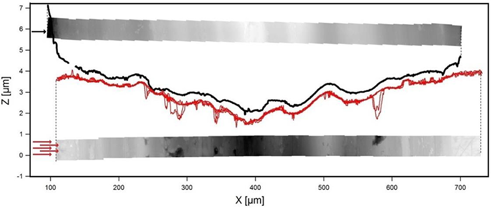
Figure 6. Profile lines perpendicular to the sliding direction of sphere (black thick line at the top) and plane (5 thin red lines at the bottom) with corresponding topography images and arrows indicating the position of the profile lines. The sphere is shown on the top in a gray scale from −2.6 μm (white) to 2 μm (black). The plane is shown at the bottom in a gray scale from −2.3 μm (black) to 0.5 μm (white). The AFM contact topographies were taken in the center of the scars on the sphere and on the plane.

A comparison of the white light measurement data with those of the AFM is shown using the example of the calotte on a sphere in Figure 7. The region scanned with AFM is shown in copper color scale. By superimposing it to the gray scale WLI image, a calibration error of the white light interferometer was found, which made it necessary to rescale the lateral dimensions of the WLI image by ca. 1%. After this rescaling, the volume measured through WLI differs by <0.5% from the volume determined by AFM. This shows that the WLI measurement data have a high accuracy. Similar results could already be shown by Wäsche et al. (2014).

FIGURE 7

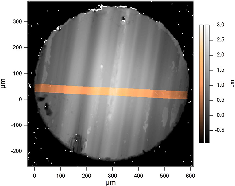
Figure 7. Superposition of two topographic images of a sphere wear calotte (R = 2 mm): total image in gray color scale acquired with a white light interferometer, section in copper color scale stitched from 26 AFM contact images.

It can be concluded that the determination of wear volumes by white light interferometry is recommendable. On the contrary, the use of AFM stitching is usually too time consuming. Yet, as shown in previous works (Wäsche et al., 2014; Cappella et al., 2015), AFM measurements are necessary when wear volumes are very small, i.e., linear wear is in the range of roughness asperities, or when the fine structure of the tracks is of interest.

Comparison of Measured and Calculated Wear

The statistical distributions of W_q and d_⊥ are useful to assess the influence of a randomly selected profile line of the wear track of a plane on the wear indicators calculated from it. The WLI measurement in Figure 5 is used as an example for this in the following. The analysis of all 3350 profile lines along Δx excluding the edge regions results in average values of 559 ± 16 μm for d_⊥, 452 ± 36 μm² for W_q and 1135 ± 65 nm for W_{l, flat}. As already stated at the beginning of section Calculation of volumetric wear, these values are strongly influenced by the roughness of the specimens; yet this influence in the determination of e.g. d_⊥ cannot be quantified. Using the maxima and minima of these distributions, the resulting mean values as well as the deviations for the exact solution of W_v according to Equation (9) and those for the approximated solutions according to Equations (10), (11), and (12) were calculated. The same procedure was used to calculate the ranges for W_{v, flat} and W_{v, ball} according to Equations (7) and (8) and for the linear wear values. W_{l, flat} and W_{l, ball} were determined through the following equations:

$\begin{array}{ll}{W}_{l,flat}\cong \frac{3W_q}{2d_{\perp }},& (14)\end{array}$

$\begin{array}{ll}{W}_{l,ball}=R-\sqrt{R^2-{\left(\frac{d_{\perp }}{2}\right)}^2}-W_{l,flat}.& (15)\end{array}$

All values are listed in Table 1. Since the WLI results have been verified through AFM measurements, the uncertainty of the measured values is well below 10⁻⁶ mm³.

TABLE 1

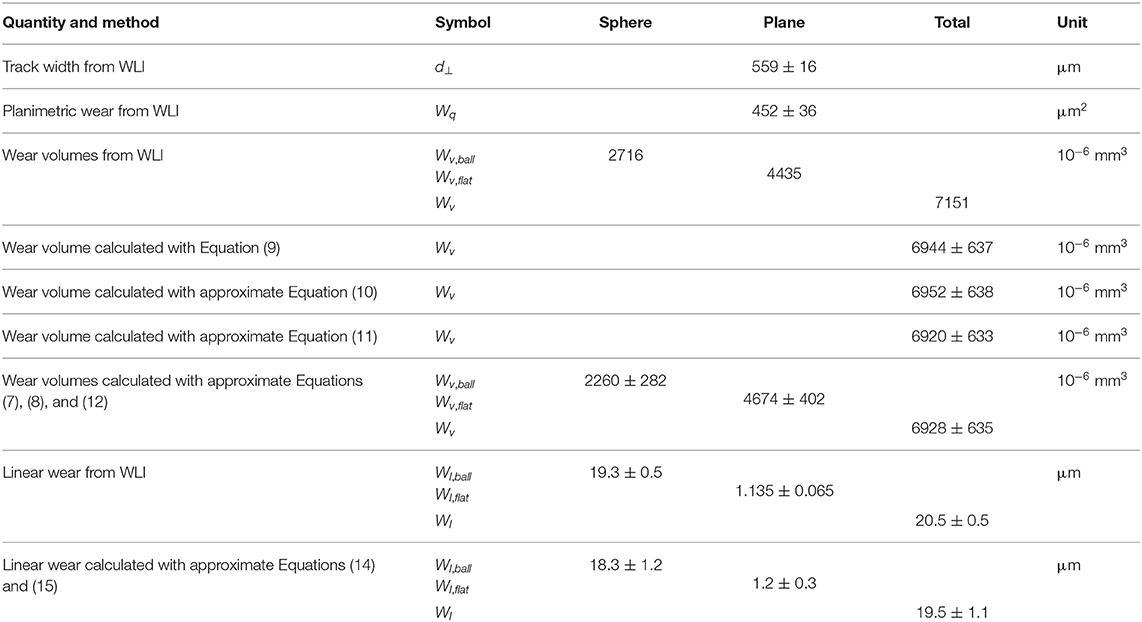
Table 1. Comparison between measured and calculated wear quantities.

The mean values of the results of the three approximated equations for W_v deviate by a maximum of 24·10⁻⁶ mm³ from the exact solution given by Equation (9), corresponding to 0.3% of the calculated volume. The standard deviation of the exact solution is 637·10⁻⁶ mm³, which, with a factor of ~27, is considerably higher than the error due to approximations.

As shown in this example, the error caused by the approximations in Equations (10), (11), and (12) can be neglected compared to the error caused by the random selection of the profile line used for calculations. By using the mean values of d_⊥ and W_q, the volume is only 2.9% smaller than the measured value. Yet, even if a profile line is selected whose d_⊥ and W_q deviate less than σ from the mean values, the error in volume can be as high as 12%. The maximum error caused by the random selection of a profile line is 25% in this example. As concerns the volumes W_{v, flat} and W_{v, ball}, the error when choosing a profile line with d_⊥ and W_q deviating less than σ from the mean values is 14 and 27%, respectively. In agreement with the analysis of the error propagation, the errors are in opposite directions (W_{v, ball} is underestimated and W_{v, flat} is overestimated) and they partially cancel out in the calculation of the total volume. The error done in the calculation of the linear wear quantities is about 10%.

The track chosen for this example has a quite regular shape. Other scars may present significant anomalies. These are described in the following section. In these cases, significantly larger standard deviations are to be expected, making the error due to the approximations even less significant.

With help of experiments performed with 100Cr6 balls on 100Cr6 planes, in which the wear volumes of the planes have been measured with WLI, the comparison just shown for one example can be extended to 102 cases. Figure 8 shows the histogram of the ratios of the calculated wear volumes of the planes, (W_{v, flat})_C, to the measured values, (W_{v, flat})_M. The calculated values were determined using a randomly selected profile line with the W_q method according to Equation (7).

FIGURE 8

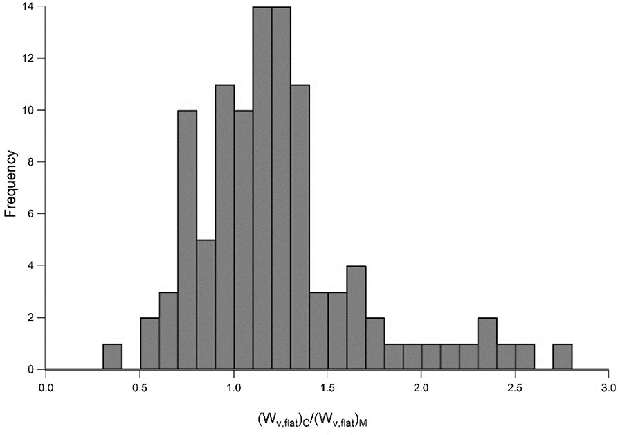
Figure 8. Histogram of the ratios of the calculated wear volumes of the planes (W_{v, flat})_C to the measured wear volumes of the planes (W_{v, flat})_M.

The histogram is not symmetric; hence, the data are not normally distributed. As in the example previously shown, the calculated volumes of the planes are usually larger than the values determined by WLI. The maximum frequency of the ratios occurs for ~1.2; the mean value is 1.13. Hence, the calculation of the volumes engenders an average error of 20%; in some cases, the error is even larger than 200%. The standard deviation (0.27) is rather large. A correlation between the deviation of the ratios from the value one and test parameters or topographic parameters, such as track width, could not be established.

In case of the ratio of the calculated total wear volumes to the measured, a similar comparison can be done only for 41 tests, since wear volumes of the spheres could not always be measured with WLI. Hence, the significance of the distribution (with a mean value of 0.964 and a standard deviation of 0.5) is not as good as for the planes. Nevertheless, it can be noticed that the error on W_{v, flat} is partially compensated by the error on W_{v, ball}.

Anomalies in the Wear Track

Anomalies in the wear track are strong deviations from the model of a uniform wear track on the plane with regular shape. Therefore, for wear tracks with anomalies, it is not possible to calculate any R′. Anomalies can occur either randomly or due to varying loading parameters, material inhomogeneities or irregular movements of the sample. In these cases, 3D measurements of the wear volume are of great advantage compared to calculations based on a few profile lines, as these randomly selected profile lines are very unlikely to be representative of the mean cross section of the track and can lead to very incorrect results. The most important anomalies are described below:

1. Irregularities of the wear calottes in the sliding direction can occur due to material breakouts or transfers, e.g., as a result of (micro) welding. Material transfer in general is actually no wear and cannot be identified, even by 3D measurements. The material adhering locally in the friction track of the plane can lead to considerable deviations when calculating volumes with the W_q method. In some cases, especially with isolated material transfers, such anomalies can be detected and taken into account.

2. Pile-ups at the edge of the wear track (e.g., due to plastic deformation or adhering wear particles) can make a track appear wider. In this case, the determination of the position of the edges, which has an important influence on the wear volume calculation, is particularly difficult.

3. Atypical wear of the ball at the edges, but not or only very slightly in the middle of the track, can make the friction track appear narrower on the plane than on the ball.

4. In case of the so-called W-shaped profile, the wear in the center of the track on the plane is very small. This leads to a different geometry of the track than the one in Figure 5 and consequently to larger errors in the calculation of W_{v, ball} and W_{v, flat}.

5. A very small wear in the range of the roughness asperities can be considered as an anomaly, too. In this case, by defining the zero value of the height in the cross-sectional profile, roughness depressions are also assigned to the worn volume and contribute to its calculated value. A better way to determine the wear volume in this case is to subtract the 3D data of an AFM measurement of the worn sample from those of the unstressed sample.

6. A last kind of anomaly is due to the fact that in some cases the linear wear W_{l, flat} depends on the position along the sliding direction. This may occur due to the wear dependence on the sliding speed or when the ball is moved not parallel to the plane, e.g., along a circular arc.

Conclusions

The current method for the analytical determination of the volumetric wear (W_v, W_{v, ball}, and W_{v, flat}) has been described in detail. The error due to inevitable approximations has been analyzed and the error propagation has been calculated, too. This analytical method (W_q method) is based on the arbitrary choice of a profile line of the wear track, usually measured with tactile techniques.

The errors due to the use of a WLI for the measurement of the profile line, to the approximations in the equations of the W_q method and to the arbitrary choice of a profile line have been assessed with help of an example. To this aim, the samples, namely a 100Cr6 ball and a 100Cr6 plane worn through an unlubricated oscillating sliding test, have been additionally measured with an AFM.

The error on the volume due to the use of a WLI resulted to be smaller than 0.5%. The error resulting from the approximations is smaller than 0.3% and can be neglected.

The arbitrary choice of a profile line for the W_q method turned out to generate the largest errors. By using the mean values of d_⊥ and W_q, the error on the volume is 2.9%. The choice of a profile line with d_⊥ and W_q differing less than σ from the mean values causes an error, which can be as high as 12%. Higher error values must be expected for scars with important anomalies, which have been listed at the end of the article.

As a conclusion, due to the large errors engendered by the arbitrary choice of a profile line for the W_q method, it is recommended to measure the volumetric wears of ball and plane and not to calculate them. For all cases in which the linear wear is comparable with the roughness of the samples, the quite time-consuming AFM stitching is necessary. Otherwise the accuracy of WLI measurements is sufficient.

Data Availability Statement

The datasets generated for this study are available on request to the corresponding author.

Author Contributions

Authors have contributed in equal measure to each part of the work and of the article.

Conflict of Interest

The authors declare that the research was conducted in the absence of any commercial or financial relationships that could be construed as a potential conflict of interest.

References

Bhushan, B. (2001). Nano-to micro scale wear and mechanical characterization using scanning probe microscopy. Wear 251, 1105–1123. doi: 10.1016/S0043-1648(01)00804-3

CrossRef Full Text | Google Scholar

Bhushan, B. (2003). Handbook of Nanotechnology. Berlin: Springer.

Google Scholar

Cappella, B., Hartelt, M., and Wäsche, R. (2015). High resolution imaging of macroscopic wear scars in the initial stage. Wear 338–339, 372–378. doi: 10.1016/j.wear.2015.07.013

CrossRef Full Text | Google Scholar

Cox, G. (2006). Optical Imaging Techniques in Cell Biology. Boca Raton, FL: CRC Press.

Google Scholar

Guilemany, J. M., Miguel, J. M., Armada, S., Vizcaino, S., and Climent, F. (2001). Use of scanning white light interferometry in the characterization of wear mechanisms in thermal-sprayed coatings. Mater. Charact. 47, 307–314. doi: 10.1016/S1044-5803(02)00180-8

CrossRef Full Text | Google Scholar

Kalin, M., and Vizentin, J. (2000). Use of equations for wear volume determination in fretting experiments. Wear 237, 39–48. doi: 10.1016/S0043-1648(99)00322-1

CrossRef Full Text | Google Scholar

Meng, H. C., and Ludema, K. C. (1995). Wear models and predictive equations: their form and content. Wear 181, 443–457. doi: 10.1016/0043-1648(95)90158-2

CrossRef Full Text | Google Scholar

Reichelt, M., and Cappella, B. (2020). Influence of relative humidity on wear of self-mated 100Cr6 steel. Wear 446–447:203202. doi: 10.1016/j.wear.2020.203239

CrossRef Full Text | Google Scholar

Wäsche, R., Hartelt, M., and Cappella, B. (2014). The use of AFM for high resolution imaging of macroscopic wear scars. Wear 309, 120–125. doi: 10.1016/j.wear.2013.11.009

CrossRef Full Text | Google Scholar

Wehbi, D., Clerc, M. A., Roques-Carmes, C., and Barquins, M. (1986). Three-dimensional quantification of wear tracks on amorphous NiB coatings. Wear 107, 263–278. doi: 10.1016/0043-1648(86)90229-2

CrossRef Full Text | Google Scholar

Yost, F. G. (1983). Two profilometric measurements of wear. Wear 92, 135–142. doi: 10.1016/0043-1648(83)90013-3

CrossRef Full Text | Google Scholar

Yu, J. X., Qian, L. M., Yu, B. J., and Zhou, Z. R. (2009). Nano-fretting behaviors of mono crystalline silicon (100) against diamond tips in atmosphere and vacuum. Wear 267, 322–329. doi: 10.1016/j.wear.2008.11.008

CrossRef Full Text | Google Scholar