 Konstantin Weller
 Silke Lipp
 Martin Röck
 Claus Matzer
 Andreas Bittermann
 Stefan Hausberger2*
- 1FVT, Forschungsgesellschaft für Verbrennungskraftmaschinen und Thermodynamik mbH, Graz, Austria
- 2Institute for Internal Combustion Engines and Thermodynamic, TUG, University of Technology, Graz, Austria
Real world emissions and energy consumption behavior from vehicles is a key element for meeting air iquality and greenhouse gas (GHG) targets for any country. While CO2 fleet targets for vehicles are defined on basis of standardized test procedures, real driving conditions manifold parameters show large variabilities. Main differences are The main differences are: driving cycle, vehicle loading and driving resistances, ambient temperature levels, start conditions and trip length, gear shift behavior of the drivers, power demand from auxiliaries, and fuel quality. For the upcoming update of the Handbook Emission Factors for Road Transport (HBEFA 4.1) we have performed analysis, measurements and simulations to simulate real world energy consumption values for 2-wheelers, passenger cars (PC), light commercial vehicles (LCVs), and heavy duty vehicles (HDVs), creating so called emission factors (EF). EFs show fuel consumption or emission level in [g/km] and [#/km] for fuel, gaseous exhaust gas components and also for the particle number (PN). EFs are provided for a lot of different traffic situations covering stop & go up to highway for different road gradient categories. EFs are different for each vehicle category and for each powertrain technology and emission standard (from EURO 0 gasoline PC to EURO VI HDV with CNG engine). To produce the EFs, vehicle tests from chassis dyno and from on-board measurements were collected in 18 independent European labs to set up models for all vehicle segments in the passenger cars and heavy duty emission model (PHEM). The models for PC and LCVs were based on weight and road load data available from the type approval test, the worldwide harmonized light vehicles test procedure (WLTP), and then calibrated in a stepwise approach to consider all influences in real world driving. Finally, the results for new vehicle fleet fuel consumption values were compared with data from the fuel consumption monitoring data base. For HDVs, the models are based on data from the development of the HDV CO2 determination method (Regulation (EU) 2017/2400, “VECTO”).
The main findings of the updates for HBEFA 4.1 are:
Exhaust pollutant emission levels from passenger cars with EURO 6d-temp type approval are below the limit values also in real driving conditions.
HDVs new vehicles real world emissions are low already since introduction of EURO VI in 2013.
Deterioration effects, ambient temperature effects on NOx from diesel cars and cold start emissions are relevant influences for the fleet average emissions.
Real world CO2 emissions are clearly higher than type approval emissions for cars and LCVs. Higher average loading, shares of vehicle mileages with roof boxes or trailers, wet road, winter tires etc. as well as real world usage of auxiliaries, such as HVAC systems are main reasons for these differences.
Introduction
Knowing the real world driving behavior, the vehicle conditions as well as the resulting energy consumption and emissions are key demands for several tasks:
• For manufacturers, the variability in possible on-board emission tests by 3rd parties in the in-service conformity (ISC) tests is relevant to safeguard their products by testing and by simulation to meet the limits in all valid tests.
• Air quality plans, e.g., defining local measures to meet NO2 air quality targets, need representative real world emission data for all relevant vehicle categories and emission classes to select proper measures and to assess their effects.
• Monitoring of regional, national and EU wide greenhouse gas targets needs accurate, real world energy consumption, and CO2 emission values of the relevant vehicle segments and powertrain technologies to assess and to select GHG reduction strategies.
• Knowing the gaps between type approval and real world driving conditions and the resulting energy consumption and emission levels helps to improve the regulations for type approval testing in the future and to improve customer information on environmental impacts of available vehicle models.
Consequently, differences between real world operation and type approval have been analyzed in many studies in the past. Deviations between emission levels in real world driving and type approval have been a known issue since the beginning of the last decade. Obviously type approval procedures with test conditions not representative for real driving and with rather large tolerances for test stand settings are the main reasons for the deviations between real world and type approval results. CO2 monitoring and limit values triggered optimization processes in the industry to exploit all options to achieve good type approval results. Examples for findings are:
The 5th EU Framework Project ARTEMIS already identified large differences in NOx emission levels in the type approval tests (ECE R49, which is a steady state test in 13 load points) and in real driving (Rexeis et al., 2005) for heavy duty engines (HDEs) with EURO II certification. Based on these findings, the HDE test conditions were steadily improved to a transient test (ETC, from EURO IV on), in addition to the inclusion of cold start for engine tests and on-board emission testing (WHTC according to Regulation (EU) No 582/2011). For HDEs, possible issues for upcoming regulations are an extension of the on-board emission testing conditions to lower loads and to include also the full cold start.
The ARTEMIS project also identified remarkable deviations in NOx emissions for diesel passenger cars for EURO 2 and EURO 3 (Boulter and McCrae, 2007). In HBEFA (http://www.hbefa.net/), version 3.1 already showed no decrease for the real world NOx emission levels for diesel cars from EURO 2 to EURO 5 (Hausberger et al., 2009). Similar results were achieved in several other studies, e.g., Ligtering et al. (2012). Since approx. 2008, the deviations between real world and type approval have been also increasing for fuel consumption and CO2 emissions, e.g., Mock et al. (2014).
To solve these problems concerning deviations between type approval values and real driving, on-board emission tests were introduced for pollutants with EURO VI for HDVs and EURO 6c for passenger cars and light commercial vehicles. In regards to energy consumption and CO2 emissions for HDV, the new CO2 determination method as described in Regulation (EU) 2017/2400 was introduced in 2018 and shall provide realistic fuel consumption values. Possible deviations are not yet known since first CO2 values according to this method have only been available since first registrations started on 1.1.2019. For passenger cars, the WLTP (Regulation (EU) 2017/1151 procedure replaced the NEDC based test procedure (Regulation (EU) 715/2007) from EURO 6c on. With this update, both the test cycle and test conditions are closer to real driving and more realistic fuel consumption values are expected compared to NEDC based values.
The main reasons for differences in the emission levels are:
a) Differences in the driving cycle (speed, acceleration, and altitude profile)
b) Differences in vehicle conditions (test mass, driving resistances, start conditions, etc.)
c) Optimizations of the vehicle control strategies for the type approval test (if applied)
For the upcoming update of the HBEFA version 4.1 extensive and systematic analysis was carried out for cars, LCVs and HDVs in order to analyze differences according to the above mentioned issues (a) to (c) to produce realistic emission factors for CO2 and pollutant emissions. As described in the abstract, EFs show the fuel consumption and emission levels in [g/km] and [#/km] for fuel, gaseous exhaust gas components as well as for the particle number (PN) for a huge set of real world traffic conditions.
The base EFs for the HBEFA are calculated using the vehicle emission model PHEM (section PHEM). The application of a model to elaborate the emission factors is inevitable, since HBEFA provides emission factors for more than 335 different traffic situations with seven different rad gradient classes. A measurement of all combinations for a representative number of vehicles would by far exceed available resources in terms of budget and time. PHEM is based on the simulation of vehicle longitudinal dynamics to compute engine power demand, engine speed and engine emission maps with exhaust gas aftertreatment modeling, e.g., Hausberger et al. (2012); Rexeis et al. (2013a), and Matzer et al. (2017). The physical character of the model requires the input both of vehicle properties and emission measurement data to set up the engine maps. The emission maps can be produced from one real world test cycle. Using this data set, type approval cycles as well as RDE routes and the HBEFA traffic situations can be simulated. The results show, inter alia, the remaining deviations between WLTP and real world fuel consumption, explain reasons for higher real world driving resistances and CO2 emissions and also indicate critical driving situations for emission levels. An important basis for the analysis was the application of an optimized processing method of the measured data. Main issues are:
✓ A correct time alignment between instantaneously measured mass flows of the exhaust gas components and the vehicles and engine operation data (torque, rpm, and velocity). A software was produced at TUG to perform these alignments together with all other evaluation steps in order to deliver an instantaneous and time aligned set of all measured quantities. In the time alignment, also the variable transport time of the exhaust gas in the vehicles' exhaust gas system and in the undiluted sample lines are corrected.
✓ An accurate assessment of the road gradient for on-road tests with sufficient time resolution as an input for the vehicle simulation of on-road tests
The paper describes the new methods developed and the findings from the analysis of real world driving conditions and emission levels. Details on the vehicles in the test sample, spread in the emission levels within the sample and related uncertainties can be found in Matzer et al. (2019).
Type Approval vs. Real World Conditions
Emission Standards in Europe for PC and LDV
Emission limits have been continuously reduced since 1972 (Regulation ECE 15/00). Since the early 1990s, the limits have been updated as “EURO classes.” Up to 2017 (for new type approvals) and up to 2018 (for new vehicle registrations), vehicles were measured in the NEDC test. With the introduction of EURO 6c, the test procedure was changed to WLTP instead of NEDC and now covers also an additional, mandatory, on-board emission test in real traffic (RDE, real driving emissions), Regulation (EC) 2017/1151.
Table 1 gives an overview of the introduction dates and related test procedures for the European emission standards for passenger cars. The dates refer to the new registration of vehicles; new type approvals were typically introduced 1 year earlier.

Table 1. Emission limits for passenger cars (DELPHI Technologies, 2018).
From EURO 1 to EURO 5, the limit values for the sum of HC and NOx were reduced by 85% (Figure 1), for particle mass from diesel cars the limits were reduced by more than 95%. Similar emission reductions were achieved for CO, HC, particle mass, and particle numbers for both, diesel (Compression Ignition, CI) and gasoline (Spark Ignition, SI) cars, e.g., Rexeis et al. (2013b). For NOx emissions from diesel cars and for CO2 emissions, however the reduction rates in real world operation were much lower than the reduction rates in the type approval tests, e.g., Ligtering et al. (2012), Mock et al. (2014), and Matzer et al. (2017).
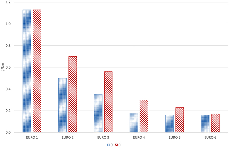
Figure 1. Limits for HC + NOx for passenger cars in Europe (DELPHI Technologies, 2018).
The reason behind the deviations between real world operation and type approval can be seen in the type approval test procedures:
• The NEDC has a large proportion of idling time, a short high speed phase and rather low accelerations. In total, this leads to much lower engine loads in the NEDC than in real world driving (Figure 2).
• The NEDC has quite low dynamic driving. Thus, accurate engine calibration for low emissions, also at higher transient driving conditions, was not needed.
• The NEDC test according to Regulation R. 83 allowed several tolerances, which were necessary for chassis dyno technologies in the early 90's but are no longer up to date, i.e., tolerances of 5% for the dyno load calibration, 5% tolerance for the coast down time, 5% for the accuracy of the CVS system and 2% for linearity of the calibration gas. With todays' much lower tolerances of the systems, it was possible to tune test stands toward the lower end of regulatory tolerances, leading to an almost 10% reduction in air and rolling resistance and a further reduction in measured emissions due to CVS and analyzer tuning.
• The temperature limits for type approval tests were defined between 20 and 30°C; only for SI cars also a low temperature test was mandatory.
• Other tolerances and flexibilities, e.g., allowing the battery to fully charge before test start.
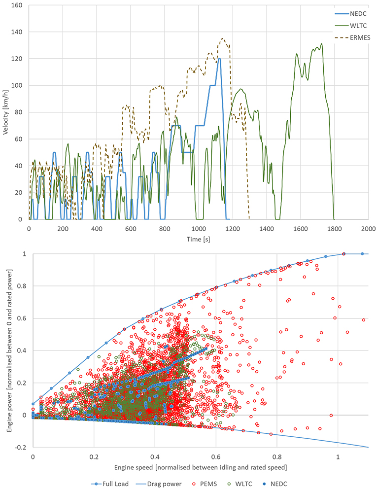
Figure 2. Comparison of NEDC, WLTC and real world cycle (Kufferath et al., 2019).
The bottom picture in Figure 2 compares the engine load points in NEDC, WLTC, and a RDE trip. The RDE trip was driven by TUG in line with the RDE regulation for EURO 6c vehicles. The load points were calculated for the “average European EURO 5 diesel car in Europe,” as defined in the HBEFA 3.3 (Matzer et al., 2017). The poor coverage of the engine map by the NEDC is clearly visible. The current chassis dyno type approval cycle (WLTC) covers the map much better, but still leaves certain aspects uncovered. However, the additional RDE test with on-board emission measurement can cover the entire engine operation range. Although a vehicle can be driven in type approval in RDE testing quite smoothly, OEMs also have to ensure that emission limits are not exceeded under demanding driving conditions. From 2019 on, ISC tests have been allowed to be performed by independent authorities, which can choose any driver behavior as long as they stay within the valid RDE trip parameters.
The measured emissions in the RDE test have to be lower than the Not To Exceed (NTE) limits, which are calculated according to Equation (1). Overall, the RDE legislation did not reduce the emission limits, but rather heavily increased the demand to meet the limits due to the much more demanding test procedure. The manufacturers now have to design the engine, the aftertreatment systems and the corresponding controllers in such a way that they meet the NTE limits under all normal driving conditions and not just under NEDC conditions.
Table 2 shows the Conformity factors for NOx and PN. The parameter margin represents additional measurement uncertainties of Portable Emission Measurement Systems (PEMS) equipment. This parameter is checked annually and may be adjusted due to the improvement of measurement accuracy. The CO emissions (carbon monoxide) for RDE shall be measured and recorded but are not limited for RDE.
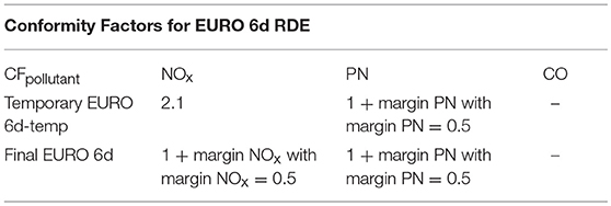
Table 2. Conformity Factors for EURO 6d RDE (Commission, 2017).
RDE test conditions were designed to cover all driving conditions relevant for air quality issues caused by traffic. To ensure that the tests are not too soft as well as to prevent unrealistic test driving, several boundary conditions for a valid RDE test regarding ambient conditions, dynamic parameters and trip parameters were defined. Most of the parameters were defined in such a way that they meet approx. 95% of the real world conditions (Kufferath et al., 2019). Table 3 shows a summary of the most important parameters for verifying the validity of a RDE test. The full description is given in Regulation (EU) No. 715/2007. The three RDE categories (Urban, Rural, and Motorway) are separated according to the vehicle's velocity with limits for minimum and maximum average velocities, distances and distance shares as well as maximum positive altitude change per 100 km.
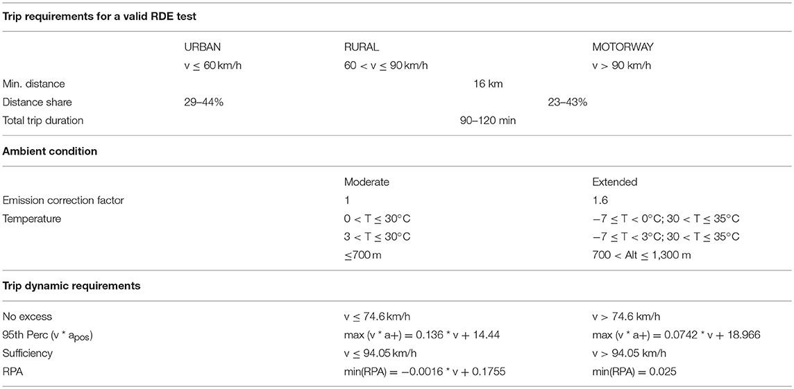
Table 3. Some boundary conditions for a valid RDE test (Commission, 2017).
Depending on temperature and altitude, two areas of the RDE test are defined. If temperature or altitude exceed certain values, an emission corrective factor is applied and the emission value is divided by 1.6 within these time steps.
Both driving behavior too aggressive and too smooth should be avoided and therefore two parameters are limited. The 95th percentile of v * a+ (velocity times positive acceleration) is limited to avoid driving that is too aggressive. The second parameter is RPA (Relative Positive Acceleration), which is used to limit driving with dynamics that are too low.
Emission Standards in Europe for HDV
Emission testing for heavy duty diesel engines started in 1992 (EURO I) with steady-state tests following the regulation ECE R-49. With the introduction of EURO III in 1999/2000, the ECE R-49 was replaced by the European stationary cycle (ESC) and complemented with the European transient cycle (ETC). There is no change regarding the test cycles up to and including EURO V, but the emission limit has decreased. EURO VI emission standards were introduced by Regulation 595/2009 and became effective from 2013.
Table 4 shows an overview of the different regulations for heavy duty vehicles (HDVs).
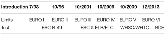
Table 4. Emission limits for heavy duty vehicles (DELPHI Technologies, 2018-2).
The current regulation EURO VI is split into two different parts:
– Type approval testing
° World Harmonized Stationary Cycle (WHSC) + World Harmonized Transient Cycle (WHTC)
° Off-cycle Emission (OCE) testing
– In-Service Conformity (ISC)
Some EURO VI provisions, like OBD requirements and OCE/ISC testing, are phased in over a period of several years. Due to measurement uncertainties for PEMS trips, the emission limit values are multiplied with a conformity factor of 1.5 for RDE testing (see COMMISSION REGULATION (EU) No 582/2011).
Although the WHTC is close to real driving (different driving conditions, high load range, transient profile, cold start), the RDE tests represented by OCE and ISC extend the test standards. The WHVC is a chassis dyno cycle which represents an engine speed and load collective near to the one of the WHTC measured on the engine test bed [Amendment 3 to UN GTR No. 4—(ECE/TRANS/180/Add.4/Amend.3)]. Variability in loading, unknown track profile, driver variability and different ambient conditions challenge the vehicles. Considering measurement results for EURO VI A–C, the regulations decrease the emissions effective compared to former EURO classes. However, the reduction of the power threshold to 10% and the upcoming inclusion of the cold start raise the requirements regarding thermal management of the exhaust aftertreatment system to a higher level.
Measurement and Simulation of Real World Emissions
The road load settings in the type approval were often even lower than the measured road load (i.e., rolling and air resistance) in the coast down test due to the tolerances allowed in the NEDC. The coast down test provides—at least when done in type approval—rather best case road load results. In real driving, several effects increase the driving resistances:
 Side wind effects
Wet road conditions
Higher rolling resistance of retrofit tires (winter tires and/or broader tire dimensions, etc.)
Roof boxes and trailers
Higher vehicle loading
Poor maintenance of tire pressure
In addition power demand from the engine in a RDE test is increased compared to the type approval on a chassis dyno due to:
+ Road gradients,
+ Power demand from auxiliaries not active on the test bed (HVAC, seat heaters, etc.).
The combination of these effects leads to higher engine loads, possibly different gear shift behavior and consequently to quite different emission levels in real driving compared to type approval, especially if compared to type approval under NEDC regulations.
In the course of the update of the HBEFA, focus was set on the design and application of vehicle simulation models for realistic driving resistances to obtain also realistic emission results.
Methods for the Assessments
For this exercise the simulation tool PHEM (section PHEM) was applied for passenger cars, LCVs and HDVs. In addition, the model VECTO (section VECTO) was used for HDVs. Both models simulate the power demand from the powertrain to follow the driving cycles.
Having a large set of chassis dyno and real world instantaneous test data for vehicles allows for a calibration of uncertain parameters. Since braking forces and engine power are known from chassis dyno and engine tests, engine fuel maps and transmission loss maps can be validated and calibrated on demand. For real world on-board tests air and rolling resistance as well as details of the power demand from auxiliaries are not exactly known and can be calibrated to meet the measured fuel consumption. Finally, fuel consumption reported by a sufficiently large sample of vehicle users can be used to calibrate average driving cycles and loading and to fine-tune auxiliary power demands and road load values in order to meet the average fuel consumption reported. These well-calibrated and well-understood datasets can then be used to simulate real world energy consumption and pollutant emissions for any driving cycles for the vehicle fleet. The methods are described in more detail below.
PHEM
PHEM (Passenger car and Heavy duty Emission Model) was developed at the IVT at TUG in the late 1990ies. Development has since then continued to go on including new technologies and improving simulation methods. A short description is given below. For example, more details can be found in Hausberger (2003), Rexeis (2009), Zallinger (2010), Hausberger et al. (2012), Luz and Hausberger (2013), and Hausberger et al. (2016).
PHEM calculates fuel consumption and emissions of road vehicles in 1 Hz for a given driving cycle based on the vehicle longitudinal dynamics and emission maps. Engine power demand for the cycles is calculated from driving resistances, losses in the transmission line, and auxiliary power demand. The engine speed is simulated by the tire diameter, final drive and transmission ratio as well as a driver gear shift model. Base exhaust emissions and fuel flow are then interpolated from engine maps. To increase the accuracy of the simulated emissions, transient correction functions are applied to consider different emission behavior under transient engine loads. Furthermore, models for the efficiency of exhaust gas aftertreatment systems are implemented. The temperatures of catalytic converters are simulated by a 0-dimensional heat balance and from the heat transfer between exhaust gas and the catalysts material and from the exhaust line to the ambient. This routine is especially important in simulating SCR systems (cool down at low engine loads) and in simulating cold start effects (Rexeis, 2009). A driver model is implemented to provide representative gear shift maneuvers for test cycles as well as for real world driving behavior.
Since the vehicle longitudinal dynamics model calculates the engine power output and speed from physical interrelationships, any imaginable driving condition can be illustrated by this approach. The simulation of different payloads of vehicles in combination with road longitudinal gradients and variable speeds and accelerations can thus be illustrated by the model just like the effects of different gear shifting behavior of drivers.
For simulation of emission factors a predefined set of “average vehicles” is elaborated for each update of the HBEFA representing average European vehicles for all relevant vehicle categories in terms of mass, driving resistances, etc. The engine emission maps and aftertreatment system parameters are gained from the huge number of instantaneous measurements in the ERMES data base. From the test data PHEM computes the engine power and then sorts the measured emissions according to engine speed and power into the engine map per vehicle. The map formats are normalized. This allows calculation of weighted average engine maps from all vehicles measured within a class (e.g., all EU 5 diesel cars). Similarly, the efficiency maps from aftertreatment systems are set up as functions of space velocity and temperature.
To assess the engine power trajectories over a test, PHEM uses a novel approach, calculating the actual engine power from CO2 and engine speed recordings (Matzer et al., 2016). Beside engine and chassis dynamometer tests, all PEMS tests can thus be used for model development—as long as emissions and engine speed are recorded and the driving cycle covers the relevant engine load areas.
VECTO
VECTO is the European Commission's official software tool for the declaration of CO2 emissions from HDVs according to regulation (EU) 2017/2400. Its development was and is funded by DG CLIMA and DG GROW. The methods and the software have been developed and programmed at TUG, e.g., Rexeis et al. (2017). Almost every new heavy-duty vehicle has to be simulated in VECTO and the resulting CO2 emissions have to be reported to the Commission. VECTO has been developed from 2011 on, based on the methods used in the model PHEM as described before. However, the software presents a completely separate development and is optimized for an accurate and reliable simulation of CO2 emissions and fuel consumption. VECTO uses target speed cycles, which lead to representative engine loads for all power to mass ratios of HDVs, since the driver model maintains inter alia full load accelerations and look ahead coasting. The model covers gear shift logics for manual transmission, automated transmission and automatic transmissions. Fuel consumption is interpolated from engine maps gained from well-defined engine certification test procedures and are corrected for transient effects, side wind effects are considered as well as axle load effects on rolling resistances.
In the course of the development of the VECTO methods, several HDVs were measured and simulated. VECTO software and data from the development process are used for the assessment of HDVs real world emissions in section Results for HDVs.
The “VECTO CO2 declaration method” is based on measurements of the individual powertrain components, e.g., combustion engine, transmission, axle gear, etc., in a standardized way. In the simulation tool the components are assembled like in the real vehicle, using certified component data as model data for the individual powertrain components. For some components, e.g., auxiliaries, a generic average power demand is applied depending on the vehicle group and mission profile. Currently all controller strategies and the driver model are generic. Then engine power and engine speed is simulated over the driving cycles using the equations of longitudinal dynamics. This provides vehicle-specific simulation results (the vehicle's resulting speed profile depends on the vehicle configuration) and at the same time comparable results among vehicle manufacturers.
VECTO is a longitudinal, backwards calculating vehicle dynamics simulation tool. The temporal resolution is about 2 Hz. The simulation results for fuel consumption and CO2 emissions have been verified in several on-road test conducted by DG JRC and different OEMs and are in the range of +/– 3% compared to the measurements. Although VECTO is already applied for HDV CO2 declaration and monitoring, the software and the test methods are permanently further developed and extended to cover new technologies and to extend VECTO to buses and to smaller lorries as well.
Handbook Emission Factors for Road Transport (HBEFA)
The HBEFA provides emission factors in [g/km] or [#/km] for passenger cars, LDVs, and HDVs on several traffic situations and different countries in Europe. Overall, the HBEFA covers more than 335 traffic situations from heavy stop & go to highway driving without speed limit, each of them for different road gradient classes, e.g., Keller and de Haan (2004). PHEM is used to simulate fuel consumption and emissions per vehicle class for all traffic situations from HBEFA for each vehicle class. The simulation results are then weighted according to the shares of the traffic situations for a specific country like Germany, for example. This paper presents the most relevant results. A more detailed description will be given in the upcoming documentation of the HBEFA 4.1.
Evaluation Methods for Instantaneous Test Data
Most relevant novel approaches are the evaluation method developed for evaluation of instantaneous exhaust gas mass emission flows and the method to calculate the road gradient trajectories.
Evaluation of exhaust gas emissions
TUG developed a comprehensive evaluation method for instantaneous measurement data, which was implemented into a software tool named ERMES Tool (Weller et al., 2016). The following chapter gives a summary on this method and shows a practical application.
Time alignment of a measured emission signal to the correct engine operating point is important for the quality of instantaneous emission data. This data is used as the base to identify emission critical situations and consequently for research and development purposes and certainly also for a correct allocation of instantaneous emissions into the engine emission maps for the model PHEM.
When emissions are measured with a PEMS (Figure 3), it can be seen that some effects distort the measurement signal on its way from the engine to the analysers. The main reasons for this are the transport time of the gas and non-ideal response characteristic of the analysers.
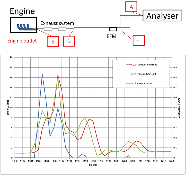
Figure 3. Schematic diagram of a PEMS and comparison of CO2 emission mass flow.
The ERMES tool corrects the main effects regarding the distortion and consequently improves the quality of the measurement signal. Below the different steps are described in the order of calculation which is reverse to the flow direction of the exhaust gas.
First, an inverse PT1 function (first order low-pass) corrects the slow response characteristic of the analysers (Position A).
Second, the algorithm shifts the corrected emission concentration about the dead time of the analysers and the constant transport time in the sample line to the sampling point (Position C). This is the position of the emission mass calculation.
The main challenge is the last part of the system, from the sampling point (Position C) back to the engine (Position E) regarding the different propagation speed of exhaust volume flow (approx. velocity of sound) and emission concentration (exhaust flow velocity). For this purpose, TUG developed a variable time shift method. This algorithm is based on emission packets that are built at every time step at position C including total exhaust mass and emission mass for every component. According to the inverse calculation direction, these packets enter the tunnel at position C and push the packets located inside the tunnel “upstream” toward the engine. Both total exhaust mass (measured by an exhaust flow meter) and emission mass of one packet stay constantly independent of the position inside the pipe. Depending on time and position, the packet volume is determined by the ideal gas equation considering various temperatures and pressures inside the system. Regarding the gas properties, exhaust gas is seen as ambient air for every packet. All emission packets leaving the tunnel per time step define the instantaneous emission mass at position E.
The graph in Figure 3 shows an extract of a test cycle as an example for a practical application of this comprehensive evaluation method compared to the constant time shift method for a vehicle test. Using the constant time shift method, the emission signal is shifted about a constant transport time for the whole cycle without paying attention to the variabilities of the transport time regarding different engine operating conditions. Applying a high quality time alignment, the CO2 signal should follow the positive vehicle acceleration. The signal of the variable time shift method (green line) correlates much better to the power signal both in low and high load phases than the result based on the constant time shift method (red line).
The same method is also applied to chassis dyno tests with CVS (Constant Volume Sampling) tunnel by adding the tunnel to the calculation as a part with almost constant gas velocity between sampling line and probe position for the analysers.
Overall, the ERMES Tool provides instantaneous exhaust mass emissions with optimized time alignment between emissions, vehicle speed, rpm, and other fast signals. This pre-processing of test data thus also improves the quality of emission maps produced from the test results since emission maxima and minima are allocated correctly to engine speed and power.
Evaluation of the road gradient trajectory for on-road trips
The accurate calculation of the road-incline is a relevant aspect in the post-processing procedure since it heavily influences the total power demand simulated by the models PHEM and VECTO in each time step.
Figure 4 shows the calculated road incline from the TUG Arzberg RDE Route based on the measured GPS altitude signal. The strong peaks are the result of a frequent change in the GPS signal's quality. In urban areas, the GPS signal could be weakened by high houses along the route. In tunnels there is no GPS signal.
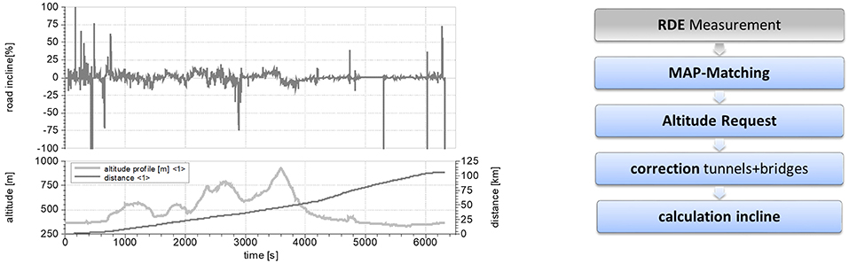
Figure 4. Workflow for incline calculation and calculated road incline.
The peaks could be limited with signal smoothing algorithms (e.g., moving average algorithm). For limiting these high peaks, the smoothing grade must be very high, therefore points with accurate GPS signals will also be smoothed. Thus, it seems impossible to use the GPS altitude signal for simulation tasks.
Figure 4 shows the workflow developed at TUG for the incline calculation. Below, the steps for this process are described.
Map matching
Map matching is the approach that takes the recorded GPS coordinates from the RDE trip and relates them to edges in an existing street graph (Jensen and Tradišauskas, 2009).
Very often differences between the original recorded route and the GPS matched route are given. For the matching, a web-based service is used. This service (TrackMatching) works with the (OpenStreetMap) road network.
The GPS points of the route are sent to (TrackMatching) with a REST API and the service sends back a list of pathways of the route. The pathways have a unique ID from the OpenStreetMap and describe attributes of the road.
Altitude request form OPEN DATA PORTAL
The returned pathways from the matching service do not provide any altitude information, so another source has to be used to gather the altitude of the route for calculating the road incline.
For the workflow, altitude data from the open data initiative “DIGITAL TERRAIN MODELS of Austria” has been used. These digital Terrain Models have been generated with precious LiDAR-measurements from Airborne Laserscan flights (Open Data Portal Österreich, 2017).
Correction at tunnels and bridges
The altitude data from these models describes the altitude of the earth's surface, so we do not get the altitude of the road in tunnels or bridges. To solve this problem of incorrect altitude, we assume that a tunnel has no additional road gradients. The positions of the tunnel are known from map matching, so the road gradient in the tunnel can be calculated as a linear function from the altitude at the beginning and at the end of the tunnel.
Calculation of the road incline
All discontinuities caused by bridges and tunnels are removed before the road incline is calculated. Despite the removed discontinuities, there can still be certain altitude signal noise. This altitude signal noise could still cause unrealistic road incline peaks. Due to this, a signal smoothing algorithm is executed in the course of the road incline calculation.
During the calculation of the road incline from a time-based signal, the distance covered is variable. Thus, the effect of the noised altitude signal is dependent on the actual distance covered. Therefore, the road incline is calculated based on constant distance segments.
The length of these distance segments is equivalent to a filter constant. A large filter constant is equivalent to a long distance segment; all peaks can be smoothed very well, but it could also cause too big a loss of road incline information. Figure 5 shows the difference between two different distance segment lengths. The light gray line in the upper diagram of this figure is the calculated road incline with a segment length of 25 m. In this case, the road incline peaks are unrealistically high.
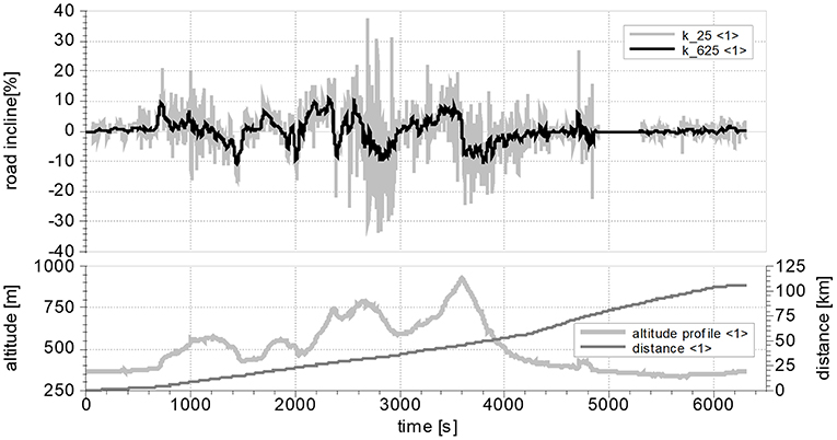
Figure 5. Comparison length distance segments.
The black line in this diagram is the road incline with a segment length of 625 m. In this case, the road incline signal has no unrealistic peaks. The maximum value of the road incline is 10%, which is also realistic.
Results for Passenger Cars
By simulation of NEDC, WLTC, real world chassis dyno cycles, RDE tests and average real world driving, in each case the unknown parameters can be calibrated to meet the measured CO2 emissions and/or fuel consumption. For EURO 6d-temp type approved vehicles the road load and test mass of the vehicles are already publicly available. Starting from these data, the following steps were taken:
1) For NEDC, the reduction of road loads and auxiliary power demand compared to the WLTC settings was assessed by adjusting these data to meet the measured NEDC CO2 emissions.
2) For RDE tests, the real world road loads and the auxiliary power demand was assessed by calibration to meet the measured CO2 emissions from PEMS tests.
3) Finally, the vehicle data set produced from calibration to meet RDE results was further calibrated to meet real world fuel consumption values reported by users (spritmonitor.de for cars and for LCVs). This final calibration provides the additional air drag due to average side wind, roof box and trailer usage as well as an assessment of real world loading and auxiliary power demand.
Steps (1), (2), and (3)—including the spritmonitor.de comparisons—were applied to a sample of four gasoline and four diesel EURO 6 cars which were tested at TUG. Characteristics of the investigated vehicles are shown in Table 5. The relative changes in road load, loading, etc. compared to type approval settings found in this analysis were then applied to the vehicle data sets from PHEM (section PHEM) describing the average vehicles per segment. All steps of this exercise are described in Opetnik (2019).
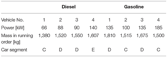
Table 5. Characteristics of the investigated vehicles for the spritmonitor.de comparisons (Opetnik, 2019).
For single vehicle simulations, the following settings were used for the simulation and the average results achieved.
The same engine fuel map, transmission model and frontal vehicle area was used in all cycles per vehicle. Gear shift logics were used as defined in the test procedure. For simulation of the RDE tests, the measured engine speed was used as model input. For the HBEFA traffic situations, the gear shift model from PHEM was applied which was designed to represent average real world behavior (Zallinger, 2010).
NEDC: For the simulation, the DIN, mass plus 100 kg, was used as defined in the regulation. Since the road load in type approval was not available, the air drag coefficient (Cd) from the WLTP-Low settings of the vehicle were reduced by 17%, the rolling resistance coefficient (fr0) by 20% to consider the tolerances in vehicle and tire selection as well as in coast down time calibration in NEDC tests. For auxiliaries, mechanical power demand of just 100 W was assumed, since the battery usually is fully charged at test start and the alternator is running at idle only in the test. A “real speed trajectory” was used instead of the target speed to mimic a driver behavior which makes use of the speed tolerances to minimize energy consumption in the test. The simulation overestimated the CO2 values stated in the vehicle certificate from type approval for the vehicles analyzed by 0 to 18%, on average by 6% (Figure 6). The overestimation in simulation may reflect average use of the tolerances, e.g., for CVS volume and CO2 analyzer accuracies in the type approval tests.
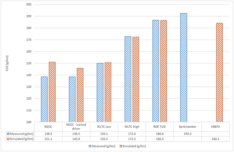
Figure 6. Average of measured and simulated CO2 emissions for the sample of four gasoline EURO 6 cars (Opetnik, 2019).
WLTC: Test mass and road loads for the WLTC were known for each of the vehicles analyzed. For auxiliaries, an average power demand of 600 W was assumed, since the WLTC corrects for differences in the battery state of charge (SOC) over the test. The CO2 values measured in WLTC-Low and WLTC-High settings were met by the simulation for the single cars with deviations between −4% and +3%.
RDE: For the simulation of the RDE test, the vehicle mass measured before the test and the road load according to the WLTC-High settings were used. Although the tested vehicles were not the worst case variants of the models, the WLTC-High resistance settings consider the increased air resistance due to the PEMS mounted and due to the winter tires used in the tests. The simulation of CO2 emissions in the RDE tests met the measured values with deviations between −6% to +9%. Deviations are assumed to result from inaccuracies from the road gradients and uncertainties from the road loads used in simulation.
Real world (HBEFA cycles): The values given below are the results from calibrating the fuel consumption simulated per vehicle model for the HBEFA traffic situation mix to the data from spritmonitor.de for each vehicle model analyzed. Spritmonitor.de provides the fuel consumption reported from the car owners in their daily use. The results thus are not based on statistics (e.g., share of winter tire driving) but represent calibration results within plausible boundaries. The vehicle mass was set to DIN mass +5% to consider extra equipment and the average loading for diesel was set to 215 kg, for gasoline vehicles to 120 kg. The different loading reflects that diesel cars are usually larger and used more frequently for long distance driving, including holiday trips etc., while smaller gasoline vehicles are used for commuting, etc. more frequently. The air drag value of the vehicles (Cd * A * δ L/2) was increased compared to the average from WLTC-High and WLTC-Low value by 8.5% to represent:
• Side wind effects, e.g., Windsor (2014),
• Approx. 5% share in mileage driven with trailers,
• 5% share driven with roof boxes,
• A higher air density than in normal conditions due to the lower average temperature (12°C average in Germany instead of 20°C).
The rolling resistance coefficient was increased against the WLTC value by 6.3%. This increase is related to following real world effects in Germany:
• 6%, if mileage driven on wet roads,
• 30% of the mileage driven with winter tires and a partly non-ideal tire pressure,
• For diesel cars an increase of a further 5% was assumed due to the selection of wider tire dimensions with possibly higher rolling resistance compared to WLTC.
Even with higher rolling resistance, fuel consumption simulated for the four diesel car models in the weighted HBEFA cycles underestimated the values reported for these vehicle models in spritmonitor.de by 14% on average. For the four gasoline cars, the deviation from the simulation against spritmonitor.de was −4% (Figure 6).
As shown later, the simulation for the average diesel car fleet matched with the fuel consumption values reported in spritmonitor.de for this average fleet almost exactly with the settings of input data described above. Therefore, we assume that weighting of the HBEFA traffic situations is not suitable for the four single diesel car models analyzed here. These rather large cars may have much higher shares of highway driving than the average car in Germany. No other explanation for the underestimation has been found yet.
The calibration for the average passenger car segments for gasoline and diesel and for EURO 0 to EURO 6d-temp used the settings gained for the HBEFA traffic situation mix for the single vehicles described above as a basis. Furthermore, the vehicle registration data on average vehicle DIN mass and engine power was used to define this input data for the PHEM models. CO2 values in NEDC type approval were taken from the CO2 monitoring data base for Germany for the average vehicle segments. All data represent the fleet averages weighted according to new registrations in Germany. The average “NEDC road load values” per segment were used as a basis, then the corrections described above were applied to produce the real-world settings. The “NEDC road load values” represent the averages of the test data available per segment from the ERMES data collection, e.g., Matzer and Hausberger (2017), with additional assumptions on the recently used tire rolling resistance coefficients and assumptions on the trends for Cd * A and RRC over time to fill gaps in the timeline down to EURO 3. Loading and auxiliary power consumption was set as described above for the single vehicle models for HBEFA settings.
For these average segments, no average test results for WLTC and RDE tests are available. Thus, the NEDC and the HBEFA traffic situation mix were simulated and compared with CO2 monitoring data as well as with spritmonitor.de data. The analysis of spritmonitor.de and CO2 monitoring data base was performed by ICCT in the course of the update to the HBEFA. Details will be reported in the upcoming documentation for HBEFA 4.1.
The simulation results for the average vehicles per EURO class match the results from CO2 monitoring and spritmonitor.de with <2% deviation without any major calibration demands. Consequently, also the ratio between real world and NEDC type approval CO2 values is very similar for simulation results with PHEM compared to spritmonitor.de data (Opetnik, 2019).
With the calibration factors elaborated in this exercise, the model data for all passenger car segments for the HBEFA shall very well represent average real-world behavior. A separate calibration routine is implemented in the HBEFA software in order to consider country specific differences based on the national CO2 monitoring data for the vehicle fleets and—if available—on specific ratios between national real world and type approval fuel consumption. The latter can reflect different speed limits and road gradient shares, among others.
Using vehicle properties calibrated with the CO2 and fuel consumption data described before, pollutant emissions are also simulated by means of the vehicle emission model PHEM. As described in section PHEM, engine emission maps are produced by filling instantaneously measured emissions into the normalized engine map formats and then averaging the maps of all tested vehicles per segment according to registration shares. For passenger cars with diesel engine and SCR catalysts an SCR model is applied in addition to consider cool down effects and NH3 dosing limitations at low exhaust temperatures. For all other passenger car segments, the engine emission maps already represent the tailpipe emission levels. For some of the segments correction functions for effects resulting from transient engine loads are applied. Since the engine maps are already filled with data from transient real-world tests, the transient correction only considers the effect of differences in the transient conditions compared to the map conditions. The correction functions are applied only for segments, for which these effects are statistically significant. The methods for transient correction are described e.g., in Hausberger (2003).
In total, more than 4000 passenger cars between EURO 0 and EURO 6d-temp have been collected in the ERMES data base. For more than 1,500 of them, real world tests are available which have been used to produce the emission factors (see Table 6). First on-board measurements were made for EURO 5 cars. For EURO 6a,b diesel cars already more than 50% of the vehicle tests were PEMS tests. This adds some complexity to measurement evaluation in taking different ambient temperature levels into consideration in a correct way, e.g. Matzer et al. (2017). Furthermore, PEMS tests provide results for CO2, CO, NOx, and PN only and the accuracy of PEMS instruments is lower than that of the lab equipment. This may especially influence PN results. Systematic analysis of the uncertainties of the PN-PEMS equipment used for the ERMES labs is not available yet.
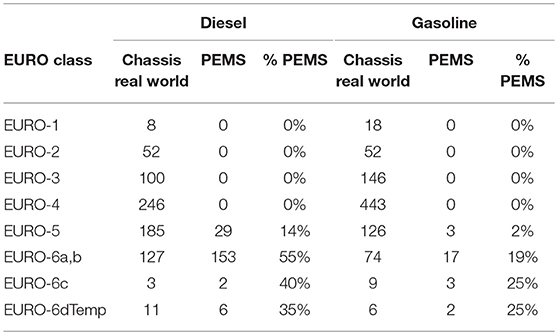
Table 6. Number of vehicles tested in chassis dyno real world cycles and on-road with PEMS available for the setup of the PHEM emission models (Matzer et al., 2019).
For LCVs, the same procedure as for passenger cars was applied, but the results cannot be presented here due to restrictions in the length of the paper.
Figures 7, 8 show the results for CO2, NOx, and PN emissions from the passenger car segments.
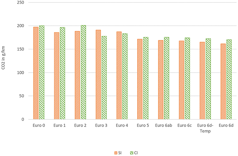
Figure 7. Average hot CO2 emission factors of the passenger car segments for HBEFA (calibrated to German driving and vehicle conditions) adapted from Matzer et al. (2019) with permission of TU Graz.
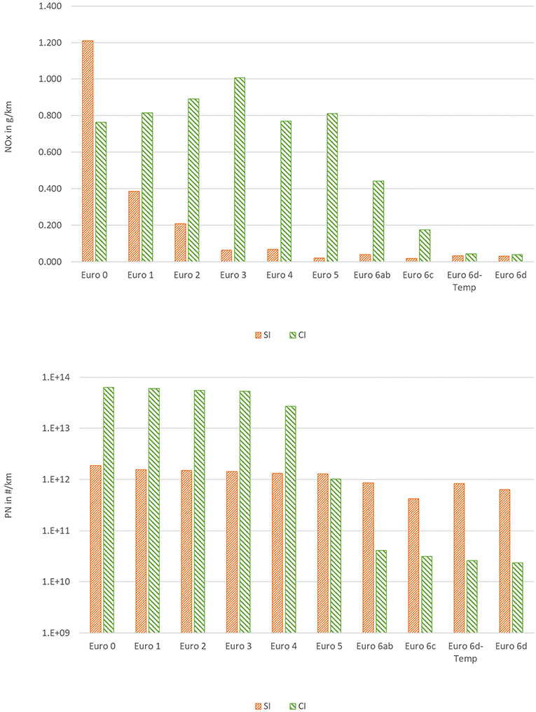
Figure 8. Average hot NOx and PN emission factors of the passenger car segments for HBEFA (calibrated to German driving and vehicle conditions) adapted from Matzer et al. (2019) with permission of TU Graz.
For CO2, the average improvements between EURO 0 and EURO 6c were some 0.5% per year. From EURO 3 to EURO 6c for diesel cars, an average 0.14% reduction was computed per anno. The rather poor reduction is also caused by the increasing sizes and weights for diesel cars (e.g., increase from 1,454 to 1,630 kg DIN mass from EURO 3 to EURO 6c).
For gasoline cars, the data shows an average reduction of −0.9% CO2 per year between EURO 3 and EURO 6c with an increase of the DIN mass from 1,165 to 1,240 kg. The real world CO2 values thus dropped much less than the type approval ones.
The recent developments in the real world NOx emission levels for passenger cars are quite positive. While diesel cars from EURO 0 to EURO 5 emitted around 800 mg NOx/km on average, the six EURO6d-temp cars tested so far led to an average hot NOx level of 44 mg/km in the HBEFA traffic situation mix. By comparison, the four gasoline EURO 6d-temp cars resulted in 33 mg/km. It is not known yet to what extent these NOx levels will change once the entire new car fleet has to meet EURO 6d-temp. However, a huge reduction in real world NOx emissions can be attributed to the new passenger car type approval system with RDE testing.
Particle mass and particle number (PN) emissions were reduced for diesel cars with the introduction of EURO 4 for a part of the fleet equipped with diesel particle filter (DPF), with the introduction of the EURO 5 limit all new diesel cars had DPFs. From EURO 5 to EURO 6 a further reduction in PN emissions was calculated for diesel cars (CI in Figure 8). This reduction may be related to better filtration technology and other technological improvements. It may also be to some extend an artifact from different measurement systems for PN. For EURO 5 vehicles, almost all PN data for the model input was gained from chassis dyno tests since only 14% of the diesel cars were tested with PEMS (Table 6) and at this time, a large number of PEMS equipment had no PN analyzer on board. For EURO 6 diesel cars, already more than 50% were measured with PEMS and most of the PEMS data includes PN results as well. Although the PN data includes uncertainties, the levels reached are very low and within the range of 3 * 1010#/km in real world driving, which is clearly below the limit value of 6 * 1011#/km. The gasoline EURO 6-d-temp vehicles tested yet showed PN levels a bit higher (8 * 1011#/km) than EURO 6c although both classes use particle filters. However, both are below the NTE limits when taking the conformity factor into consideration. Compared to EURO 3 diesel cars without DPF, EURO 6 gasoline cars have 98% lower PN emissions, diesel cars show a −99.95% reduction in PN vs. the EURO 3 diesel. Thus, the introduction of particle filters reduced particle emissions from cars to almost zero impact. For CO and HC similar reductions of emission levels were computed.
Results for HDVs
The methods applied for HDVs were similar as those applied for cars but without the possibility to calibrate the model input data in order to meet fuel consumption with a large set of user information. From 2020 on the availability for HDV data is expected to improve significantly, since the CO2-emissions and other relevant parameters computed by VECTO will be available from the monitoring activities for new registered HDVs according to Regulation (EU) 2018/956.
In order to be able to produce real world fuel consumption in the new version of the HBEFA (4.1), the vehicle specifications for all emission standards (EURO 0–EURO VI) have been updated for the PHEM models as compared to version 3.2. Model input for typical EURO VI configurations was derived from tests and data collection performed during the development of the HDV CO2 determination method (Regulation (EU) 2017/2400, “VECTO”). Based on the EURO VI models, the following vehicle components were adapted for the different vehicle generations from EURO V to EURO 0:
• Vehicle weight
• Engine Power
• Air drag coefficients
• Auxiliaries
• Axle ratio
• Rolling resistance coefficient (RRC)
• Transmission type
• Specific fuel consumption maps
Table 7 shows the changes in these specifications from EURO 0–EURO VI for a tractor trailer combination with a gross vehicle mass (GVM) between 34 and 40 tons.
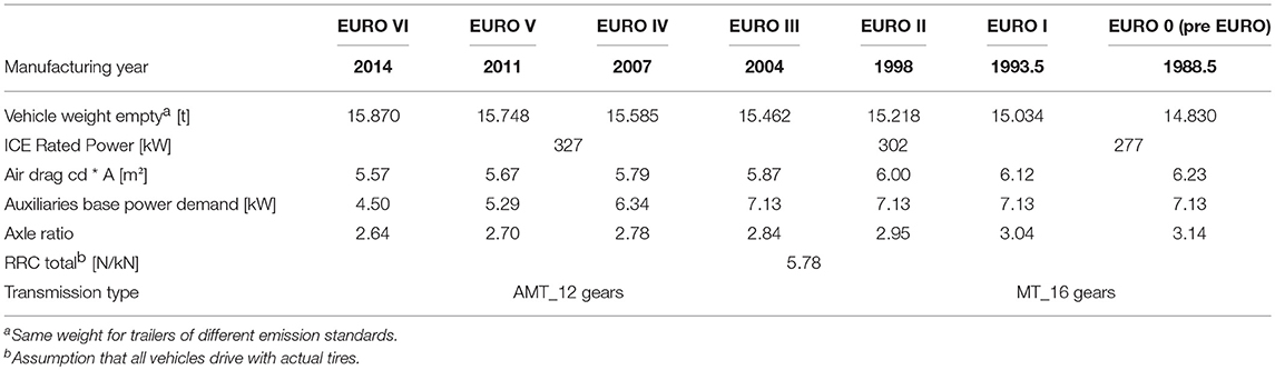
Table 7. Vehicle specification depending on generations (emission standards) (Matzer et al., 2019).
The differentiation of engine specific fuel consumption depending on the vehicle generation was adjusted by correction factors using the EURO VI map as a base. The Euro classes IV and V were further subdivided according to emission reduction technologies EGR (Exhaust Gas Recirculation) and SCR (Selective Catalytic Reduction), since these technologies have different effects on fuel consumption. Table 8 shows the differences in fuel consumption depending on the engine generation. Rexeis and Kies (2016) describes the different factors in detail.

Table 8. Fuel consumption ratios of engine generations (Matzer et al., 2019).
However, EURO VI engines show also significant differences in the fuel consumption dependent on the engine size regarding WHTC results. The fuel consumption rises with a decreasing rated engine power. A correction of engine size was thus applied according to a regression function for EURO IV to EURO VI engines. For engine generations up to EURO III, the functions were taken from HBEFA 3.3 (Rexeis et al., 2005) and adapted to current maps. This allows the usage of an average fuel consumption map for all engine power classes per EURO class.
As already mentioned, there are many influences in real world driving, which have a significant effect on fuel consumption and thus on CO2 emissions. Since it is practically impossible to measure all these effects for the large number of vehicle segments, VECTO models were used to validate fuel consumption of the HBEFA 4.1 models which have been simulated with PHEM (see section PHEM). A validation based on fleet data is currently not possible, since the regulation on monitoring and reporting of fuel consumption and CO2 emissions started on January 1, 2019. VECTO (see section VECTO) is the official tool for the certification of CO2 emissions of HDVs in Europe and representative for real world conditions.
A comparison between VECTO and PHEM for a EUVI tractor trailer on the VECTO mission profiles (long haul and regional delivery) was made and showed a good correlation. The deviations of 0.8% for the long haul cycle and 1.5% for the regional delivery cycle result mainly from different transmission models for VECTO and PHEM.
A simulation of the HBEFA 4.1 highway cycle mix for Germany in comparison with the VECTO Long haul cycle showed a 6% higher fuel consumption for HBEFA 4.1 cycle mix. Which of the cycles is more representative for real driving remains to be seen. Future CO2 monitoring activities for HDVs—which will be similar to the ones established for LDVs—will allow for a similar comparison between certified and real world fuel consumption, as shown for cars in section VECTO.
Figure 9 summarizes fuel consumption results for all EURO classes of the tractor trailer with 34–40t GVM and a payload of 50%. The results correspond to the HBEFA 4.1 values with the average weighting for German motorways. The technological developments from EURO 0 to EURO VI as described in Figure 9 have a positive influence on fuel consumption, but for EURO 0 to EURO II improved engine technologies are most significant (turbocharger, charge air cooler, etc.). They lead to a reduction in fuel consumption by approximately 10%. Due to the continuous reduction of nitrogen oxides (NOx) emissions and the introduction of more demanding test procedures, fuel consumption more or less stagnated between EURO II and EURO IV despite improved vehicle specifications. Technologies used for NOx reduction, such as later injection timing or EGR, obviously showed a significant negative impact on engine efficiency. The need for an inefficient setting of the combustion parameters was clearly reduced by the introduction of SCR systems from EURO V on, since these systems allow higher raw exhaust NOx emissions.
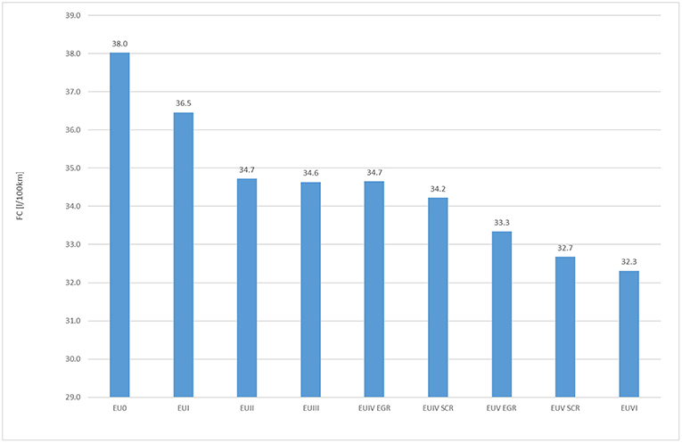
Figure 9. Specific fuel consumption values of the HBEFA 4.1 depending on the vehicle generation for a tractor trailer on an average German motorway adapted from Matzer et al. (2019) with permission of TU Graz.
This chapter shows a comparison between HBEFA 3.3 and the new HBEFA 4.1 emission results. The different results are caused by various reasons:
• Updated data base with 25 vehicles measured in RDE and 8 on chassis dyno
• Vehicle specifications
• Update of driving cycles
EURO VI HDVs showed low emissions in almost all driving situations. Only in longer low load driving, cool down effects in the exhaust aftertreatment system led to a drop in NOx conversion efficiency. At exhaust temperature below approx. 200°C, no AdBlue dosing is possible. After approx. 30 min without AdBlue dosing, the NH3 storage is exhausted and no NOx conversion is possible unless AdBlue dosing is started again. To cover these special operating conditions, HBEFA 4.1 introduced a new traffic situation called “Stop & Go 2.” Compared to the traffic situation “Stop & Go,” this cycle extends the low load phases.
Since NH3 storage in the SCR catalyst has a big influence on NOx emission reduction, the SCR model in PHEM based on temperature and space velocity inside the catalyst was extended with functions for AdBlue injection, NH3 storage capacity as function of the temperature of the catalyst and influence of NH3 storage on the NOx conversion rate.
The weighted average of all HBEFA traffic situations was computed for HDVs from EURO 0 to EURO VI. Figure 10 shows the results as an example for the tractor trailer combination (34–40t, half load). NOx emissions have constantly decreased over the last years due to stricter limits and the implementation of new test cycles, which cover a broader area of the engine map. EURO IV and EURO V brought an effective reduction with a widespread application of SCR catalysts, but the introduction of EURO VI limits the emissions to a minimum. Of course, the new chassis dyno cycle WHTC is a challenge, but the introduction of RDE tests leads to an effective improvement of the emission performance of EURO VI vehicles.
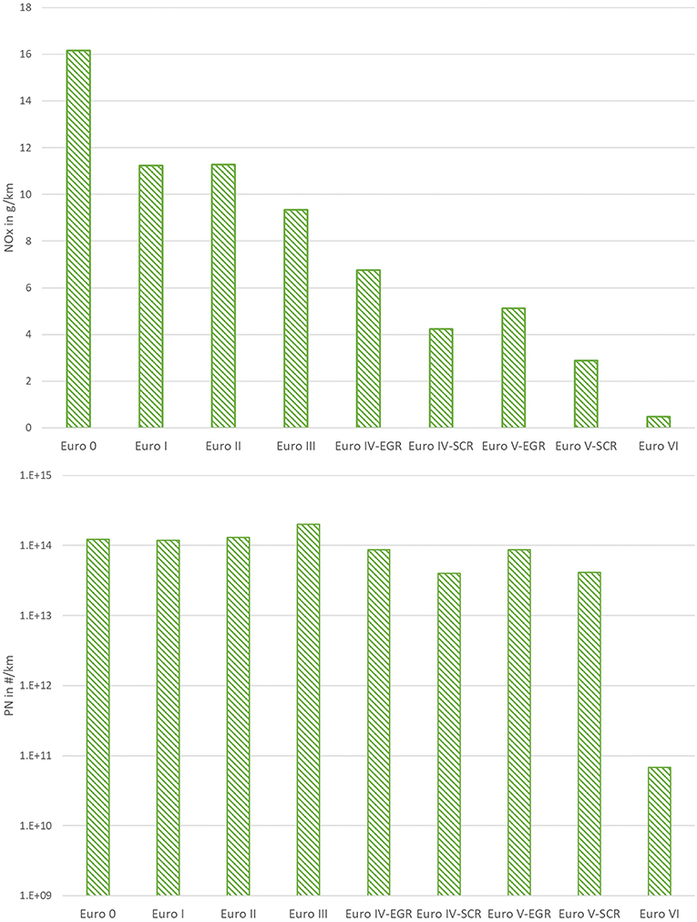
Figure 10. Average hot NOx and PN emission factors for HDV TT 34–40t for HBEFA adapted from Matzer et al. (2019) with permission of TU Graz.
Figure 10 shows the development of PN emissions of HBEFA. Up until EURO VI, only PM was limited and consequently PN emissions stayed more or less constant. The introduction of additional PN limits led to the application of DPF for all vehicles and to a huge decrease in PN emissions.
BEV and PHEVs
The simulation tool PHEM (section PHEM) needs additional input parameters for the BEV and HEV simulation as shown in Table 9. The BAT file includes information concerning the battery, such as the numbers of cells, the capacity of the battery and so on. The EMO file describes the efficiency of the electric motor over the engine speed and power and the full load characteristic. The STE file describes the parameters for the control strategy of hybrid vehicles.
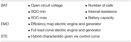
Table 9. Additional Input files for BEV and HEV for PHEM.
The aim of the HEV control strategy is to minimize fuel consumption and emissions. The following effects are simulated:
• Recuperation of braking energy up to a chosen SOC max
• Engine stop at zero power demand as long as SOC actual > SOC min
• Electric driving is preferred as long as SOC actual > SOC min
• Selection between electric driving, electric assistance and driving with combustion engine only
For the selection of the driving mode, the overall best efficiency over a trip is relevant. As key control parameter, PHEM calculates a so called efficiency factor Ke for each time step. The following equation is used:
The efficiency factor for assisting and charging (shown in the following equations) is calculated and compared.
“Assisting” is allowed only for Ke_assist values below the threshold curve, generation of electric energy is allowed for Ke_generate above the thresholds, otherwise no efficiency increase is given in comparison to driving with combustion engine only.
The vertical line in Figure 11 is a schematic picture of the decision making process in a time step. In this example, the selection would be generating since it has a larger distance to the threshold curve.
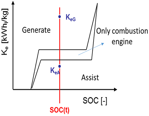
Figure 11. STE curve for the hybrid control strategy in PHEM (Matzer et al., 2019).
The dependency of the STE curve on SOC ensures that toward SOC Min generating is preferred and that SOC Min is not exceeded. Consequently, electric drive is preferred toward SOC Max, to keep capacity in the battery available for possible regeneration at braking events.
The vertical height of this curve is found by real world cycle simulations (Lipp et al., 2017).
The limits for the factors are defined in the STE curve shown in Figure 11.
Validation with measurements on a BEV
For the efficiency map validation of the electric vehicle, a BEV car (C segment) was measured and simulated. The measurements were done on the chassis dynamometer and on the road on the standard RDE route used by TUG. Table 10 shows the vehicle data of the measured BEV.
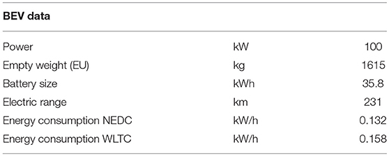
Table 10. BEV data according to type approval (Matzer et al., 2019).
During the measurements on the dynamometer, voltage and electrical current where logged to get the electrical fuel consumption for each cycle. After that the cycles were simulated with a BEV model in PHEM and the electrical consumption was compared as shown in Table 11.
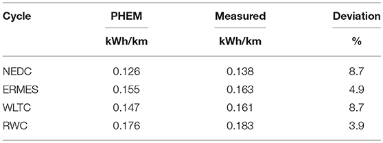
Table 11. Electrical consumption measured and simulated at TUG (Matzer et al., 2019).
For the NEDC, the highest deviation is about 9%. For more dynamic cycles, like ERMES and RWC, deviation decreases. It has to be noted that the efficiency map and the transmission loss maps were gained from generic models. Thus, the deviations between measurement and simulation are in the expected range. An accurate calibration to the single measured BEV was not undertaken, since it is not clear, whether the vehicle's efficiency is better or worse than the average BEV. The PHEM model was used for further BEV simulations employing the settings used for this comparison.
Simulated Emissions for BEV and PHEV With PHEM
For EVs, the simulated fuel consumption is shown as kWh/km in the result file of PHEM. For the PHEV simulation, emissions and energy consumption are computed for electric driving in charge depleting mode and for hybrid driving in charge sustaining mode. The two results are weighted according to the electrical driving share as shown in the following equation:
Electrical driving share
The electrical driving share (KEV) is needed for the calculation of the weighted emissions for PHEVs. To get a simple dependency between electrical driving share and average speed for application in the HBEFA 4.1, the method described below was used.
The first step was to define the relevant model input data for the average PHEV. The average PHEV was set up according to the current PHEVs on the market by weighting the vehicle data according to the sales numbers. This results in an average electric range of 43 km, a vehicle mass of 1,738 kg (curb weight), an engine power of 123 kW and an electrical power of 79 kW. Details can be found in Lipp et al. (2017).
The second step was to find typical mission profiles that represent urban, rural and motorway driving for different trip length. A generic set of trips between 20 and 300 km length were produced. The missions started and ended in urban areas. The distances driven on motorway and rural roads were increased more than the urban mileage for increasing trip lengths. The distance of the profiles varied. These mission profiles were simulated with different start SOCs to get the share of electrical driving for different distance classes and for different start SOC classes. For the distribution of the SOC at trip start, no statistical data could be found—this is why TUG estimated that about 40% of the rides are done with a start SOC of 80%. Together, with an average distance distribution for cars in Germany, the weighted electrical driving share was computed from the matrix of distance and SOC start classes. With average speeds for urban, rural and motorway driving, the electric driving share was gained as function of the average velocity (Lipp et al., 2017).
Figure 12 shows the distribution calculated for the electrical driving share for the HBEFA 4.1 cycles.
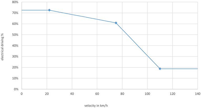
Figure 12. Electrical driving share over average velocity calculated for the average PHEVs (Lipp et al., 2017).
Figure 13 shows the simulation results for CO2 emissions for the HBEFA 4.1 cycles for a traffic situation mix for Germany (the blue bars in the figure) for Diesel, Gasoline, BEV, PHEV Diesel and PHEV Gasoline for the emission class EURO 6ab. Since HBEFA represents the fleet average vehicles, the diesel cars are larger than gasoline cars. For a comparison of the propulsion system, CO2 emissions were simulated also for vehicles with different propulsion concepts installed in the same vehicle body (all as C segment; orange bars).
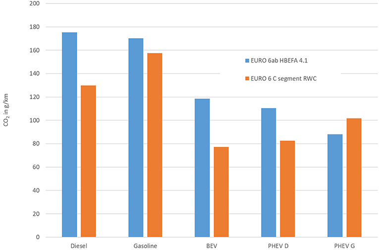
Figure 13. Simulated CO2 emissions adapted from Matzer et al. (2019) with permission of TU Graz.
An overview of the vehicle data used in the simulation is given in Table 12. For the EURO 6ab vehicles simulated in the HBEFA 4.1 cycles, the diesel-driven vehicle has the highest CO2 emissions. For the EURO 6 C-segment vehicles simulated in the RWC (Real World Cycle), the gasoline driven vehicle has the highest CO2 value. The RWC is a cycle generated by TUG which represents the standard RDE route driven for the RDE measurements by TUG. The cycle meets the boundary conditions for a valid RDE trip.
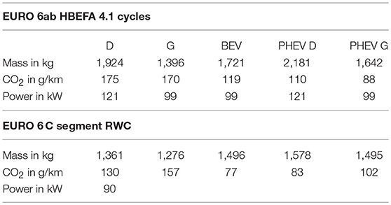
Table 12. Overview of vehicle data (Matzer et al., 2019).
For illustration, the CO2 WTT (Well To Tank) emissions allocated to electricity consumption were calculated by multiplying the specific electric energy consumption [kWh/km] with a specific CO2-factor of 480 g/kWh for the European power plant mix. Since the study is not focusing on life cycle analysis, WTT emissions of all other fuels were not considered.
As shown in Table 12, the biggest difference between the vehicles for the HBEFA 4.1 study and the one with the same segment concerns the vehicle weight. This fact leads to different CO2 emission levels between the propulsion concepts.
Basically, the model PHEM can also calculate the pollutant emissions for HEVs and PHEVs from the simulated engine power and engine speed as described for conventional vehicles before. Using the average engine emission maps from conventional vehicles to simulate pollutant emissions for HEVs leads to artifacts, since engine calibration for HEVs and PHEVs is different to conventional drive trains due to different engine operation areas. For HBEFA 4.1, the HEVs get the same pollutant emission values per traffic situation as conventional vehicles. BEVs and PHEVs in electric mode certainly have zero emissions. A separate set of engine maps fitting to HEV strategies may be elaborated if more test data is available in future.
Summary
Comparisons of real driving emissions and type approval emissions often show that the emissions measured on the streets are higher than those measured in the laboratory. Several effects—explained in more detail in this paper—lead to higher driving resistance factors in real driving, higher power demands and different engine load points compared to type approval tests. For realistic emission results, the focus was on the design and application of vehicle simulation models that consider all relevant effects in real world driving.
For the simulation models, and especially for the creation of emission maps, the time alignment of emission mass flows to the correct engine operation points is essential. For the emission simulation, a longitudinal dynamics model (PHEM) is used. The quality of the road gradient signal is essential for the correct calculation of the power demand. TUG developed a software tool (ERMES) that determines both the correct time aligned instantaneous exhaust gas mass emissions flows and the road gradient trajectories.
For four diesel and gasoline passenger cars, the NEDC, WLTC, real world chassis dyno cycles, RDE tests and average driving in Germany were simulated and calibrated using measurement data. The models calibrated to average German driving conditions were then used as inputs to simulate representative real world driving cycles from HBEFA 4.1. The results for average real world driving with passenger cars in Germany are:
• CO2 improvements for diesel cars between Euro 0 und EURO 6c were an average of between 0.14% per year, for gasoline cars improvements were 0.9% per year. The poor reduction concerning diesel cars is caused by, to a large extent, increasing vehicle sizes and weights.
• Diesel cars from EURO 0 to EURO 5 emitted around 800 mg NOx/km, the current EURO 6d-temp cars have an average NOx level of 44 mg/km. Euro 6d-Temp gasoline cars are on a similar level. To which extent these NOx levels will change once the entire new car fleet has to meet EURO 6d-temp remains to be seen. The reduction of NOx emissions can be attributed to the new type approval test with RDE testing.
• With the introduction of DPFs, emitted PN have been reduced. The comparison of cars with DPF (e.g., Euro 6) to cars without DPF (e.g., EURO 3) shows a reduction of 99.95%. The particle count of gasoline passenger cars showed slightly higher PN levels than diesel cars with DPF.
Fuel consumption values of HDVs show an average annual reduction of approx. 0.7% between EU0 and EURO VI. EURO VI vehicles show CO2 emissions that are 2% lower than those of EURO V vehicles. CO2 emissions of the generations EURO II to EURO IV are 7% higher and EURO I and older vehicles emit 13 and 18% more CO2 emissions compared to EURO VI. Compared to cars and LCVs, results for HDVs may be more uncertain, since there is no European wide monitoring data base available for HDVs yet. This will change in the future due to the regulation on monitoring and reporting of fuel consumption and CO2 emissions adopted by the EU commission, which came into effect on January 1, 2019. This makes it possible to validate future vehicle models based on this data.
For HDV, the emission reduction for NOx has become more and more effective over the last years due to stricter limits and driving cycles, which covers a broad area of the engine map. The introduction of EURO VI led yet to another reduction in emissions levels, mainly due to the implementation of on-board emission tests. PN emissions with EURO VI have also been drastically reduced due to the introduction of PN limits and consequently the application of all vehicles with DPF.
Derived from conventional driven vehicles for HBEFA 4.1 PHEV and BEV, simulation models were created to show the potential for fuel consumption reduction between the different driving concepts. For the simulation models, some additional parameters for electrical components of hybrid cars and a control strategy for handling the driving mode of those vehicles were introduced. Furthermore, the distribution for the electrical driving share depending on the average cycle velocity was estimated.
The simulated CO2 results for a traffic situation mix in Germany shows a CO2 saving potential of about 37% for the PHEV diesel compared to the conventional driven diesel passenger car (EURO 6ab) provided an average EU mix is used to allocate CO2 emissions to electric energy consumption.
Author Contributions
KW, SL, MR, CM, and AB are Ph.D. students at the University of Technology on the Institute of internal combustion engines and thermodynamics at the department Emission Research. Our Supervisor is SH, who leads this department.
Conflict of Interest Statement
The authors declare that the research was conducted in the absence of any commercial or financial relationships that could be construed as a potential conflict of interest.
Abbreviations
a, Acceleration; AMT, Automated Manual Transmission; Approx., approximately; AT, Automatic Transmission; BEV, Battery Electric Vehicle; CB, City Bus; cd, Drag coefficient; CF, Conformity factor; CNG, Compressed Natural Gas; CO, Carbon monoxide; CO2, Carbon dioxide; corr, Corrected; CVS, Constant Volume Sampling; D, Diesel; DG, Director general; DPF, Diesel Particulate Filter; e.g., Example given; EC, Emission Concentration; EC, Energy Consumption; EGR, Exhaust Gas Recirculation; el., Electric; ELR, European Load Response (ELR); EMF, Emission mass flow; E-Motor, Electric Motor; ERMES, European Research on Mobile Emission Sources; ESC, European Stationary Cycle; ETC, European Transient Cycle; etc., Et cetera; ExMF, Exhaust mass flow; FC, Fuel Consumption; G, Gasoline; GHG, Greenhouse Gas; GVM, Gross Vehicle Mass; HBEFA, Handbook Emission Factors for Road Transport; HC, Hydrocarbon; HD, Heavy Duty; HDE, Heavy Duty Engine; HDV, Heavy Duty Vehicle; HEV, Hybrid Electric Vehicle; HVAC, Heating, Ventilation, and Air Conditioning; i.e., Id est; ICCT, International Council on Clean Transportation; ICE, Internal Combustion Engine; ISC, In-service-conformity; IVT, Institut für Verbrennungskraftmaschinen und Thermodynamik; Ke, Efficiency factor; JRC, Joint Research Center; LCV, Light Commercial Vehicle; LDV, Light Duty Vehicle; max., Maximum; meas, Measured; min., Minimum; MT, Manual Transmission; NEDC, New European Driving Cycle; NH3, Ammonia; No., Number; NO2, Nitrogen dioxide; NOx, Nitrogen oxide; NTE, Not To Exceed; OBD, On-Board Diagnostics; OCE, Off-cycle Emission; OEM, Original Equipment Manufacturer; P, Power; PC, Passenger Car; PEMS, Portable Emissions Measurement System; PHEM, Passenger car and Heavy duty Emission Model; PHEV, Plug-in Hybrid Electric Vehicle; PN, Particle Number; RDE, Real Driving Emissions; RPM, Rounds per minute; RRC, Rolling Resistance Coefficient; RPA, Relative Positive Acceleration; RWC, Real World Cycle; SCR, Selective Catalytic Reduction; SoC, State of Charge; TT, Tractor trailer; TTW, Tank To Wheel; TU Graz/TUG, Technische Universität Graz; Ubus, Urban bus; ugas, ratio of density between emission component and exhaust gas; v, Velocity; VECTO, Vehicle Energy Consumption Calculation Tool; W, Energy; WHSC, World Harmonized Stationary Cycle; WHTC, World Harmonized Transient Cycle; WHVC, World Harmonized Vehicle Cycle; WLTC, Worldwide harmonized Light vehicles Test Cycle; WLTP, Worldwide harmonized Light vehicles Test Procedure; WTT, Well To Tank; xEV, Vehicle with an electrified propulsion system; Δm, Mass difference.
References
Boulter, P., and McCrae, I. (2007). ARTEMIS, Assessment and Reliability of Transport Emission Models and Inventory Systems. DG TREN Contract 1999-RD.10429WP400. TRL Report UPR/IE/044/07. Wokingham, Berkshire.
Commission (2017). Regulation (EU) 2017/1151. Available online at: https://eur-lex.europa.eu/legal-content/DE/TXT/?uri=CELEX%3A32017R1151
DELPHI Technologies (2018). “Worldwide emission standards,” in Passenger Cars and Light Duty Vehicles 2018/2019. Available online at: https://www.delphi.com/newsroom/press-release/delphi-technologies-launches-26th-worldwide-emissions-standards-book# (accessed July 18, 2019).
DELPHI Technologies (2018-2). “Worldwide emission standards,” in On and Off-Highway Commercial Vehicles 2018/2019. Available online at: https://d2ou7ivda5raf2.cloudfront.net/sites/default/files/2019-05/2018-2019%20Heavy-Duty%20%26%20Off-Highway%20Vehicles.pdf (accessed July 18, 2019).,
Hausberger, S. (2003). Simulation of Real World Vehicle Exhaust Emissions. Graz: Graz University of Technology. VKM-THD Mitteilungen Heft/Volume 82. ISBN 3-901351-74-4.
Hausberger, S., Lipp, S., and Matzer, C. (2016). “Anforderungen durch die kommende real drive emissions (RDE) gesetzgebung für PKW,” in ÖVK Vortrag (Graz).
Hausberger, S., Rexeis, M., and Luz, R. (2012). “New emission factors for EURO 5 & 6 vehicles,” in 19th Transport and Air Pollution Conference (Thessaloniki).
Hausberger, S., Rexeis, M., Luz, R., and Zallinger, M. (2009). Emission Factors from the Model PHEM for the HBEFA Version 3. Graz: Graz University of Technology. Report I-20/2009 Haus-Em 33/08/679.
Jensen, C., and Tradišauskas, N. (2009). “Map matching,” in Encyclopedia of Database Systems. doi: 10.1007/978-0-387-39940-9_215
Keller, M., and de Haan, P. (2004). Handbuch Emissionsfaktoren des Straßenverkehrs 2.1. Zurich: Infras. UFOPLAN-Ref. 29843100/02.
Kufferath, A., Naber, D., Hausberger, S., and Steven, H. (2019). “EU6d - analyse der randbedingungen und ableitung der emissionsauswirkungen am beispiel des weiterentwickelten diesel powertrain,” in 40th Vienna Motor Symposium (Vienna).
Ligtering, N., Kadijk, G., and van Mensch, P. (2012). Determination of Dutch NOx Emission Factors for Euro-5 Diesel Passenger Cars. The Hague: TNO. Report 2012 R11099.
Lipp, S., Hausberger, S., and Schreiber, L. (2017). “Measurement and simulation of hybrid and plug in hybrid vehicles for the handbook of emission factors,” in 22nd Transport and Air Pollution Conference (Zurich).
Luz, R., and Hausberger, S. (2013). User Guide for the Model PHEM, Version 11.2. Graz: Graz University of Technology.
Matzer, C., and Hausberger, S. (2017). Update of Emission Factors for EURO 4, EURO 5 and EURO 6 Diesel Passenger Cars for the HBEFA Version 3.3. Graz: Graz University of Technology. Report I-09/17/ CM EM 16/26/679.
Matzer, C., Hausberger, S., Lipp, S., and Rexeis, M. (2016). “A new approach for systematic use of PEMS data in emission simulation,” in 21st Transport and Air pollution Conference (Lyon).
Matzer, C., Hausberger, S., Rexeis, M., Opetnik, M., Ramsauer, M., Mogg, O., et al. (2017). “Update of emission factors for EURO 6 diesel passenger cars for the HBEFA,” in 22nd Transport and Air Pollution Conference (Zurich).
Matzer, C., Weller, K., Dippold, M., Lipp, S., Röck, M., Rexeis, M., and Hausberger, S. (2019). Update of Emission Factors for HBEFA Version 4.1. Graz: Graz University of Technology. Report I-05/19/CM EM-I-16/26/679
Mock, P., Tietge, U., Ligtering, N., Lambrecht, U., Kühlwein, J., Riemersma, I., et al. (2014). From Laboratory to Road, A 2014 Update of Official and “Real-World” Fuel Consumption and CO2 Values for Passenger Cars in Europe. Berlin: ICCT.
Open Data Portal Österreich (2017). Digitale Geländemodelle von Österreich. http://data.opendataportal.at/dataset/dtm-austria (accessed December 7, 2018).
Opetnik, M. (2019). Messung und simulation von Euro 6 Otto-PKW emissionen für das handbuch emissionsfaktoren des Straßenverkehrs (Master thesis). Graz: Graz University of Technology.
Rexeis, M. (2009). Ascertainment of real world emissions of heavy duty vehicles (Ph.D. thesis). Graz: Graz University of Technology.
Rexeis, M., Hausberger, S., Kühlwein, J., and Luz, R. (2013a). Update of Emission Factors for EURO 5 and EURO 6 Vehicles for the HBEFA Version 3.2. Graz: Graz University of Technology. Report I-31/2013/ Rex EM-I 2011/20/679.
Rexeis, M., Hausberger, S., Riemersma, I., Tartakovsky, L., Zvirin, Y., van Poppel, M., et al. (2005). Heavy Duty Vehicle Emissions. Graz: Graz University of Technology. Report I 02/2005/Hb 20/2000 I680.
Rexeis, M., and Kies, A. (2016). Ertüchtigung von VECTO zur Berechnung des Energieverbrauches von Schweren Nutzfahrzeugen vor Erstzulassung 2018. Graz: Graz University of Technology. Report FVT-097/16 Rex Em 15/25-1/6790.
Rexeis, M., Kühlwein, J., Luz, R., and Hausberger, S. (2013b). Update of Emission Factors for EURO 5 and EURO 6 Passenger Cars for the HBEFA Version 3.2. Graz: Graz University of Technology. DG JRC Contracts N°108919 and N°108921.
Rexeis, M., Quaritsch, M., Hausberger, S., Silberholz, G., Steven, H., Goschütz, M., et al. (2017). VECTO Tool Development: Completion of Methodology to Simulate Heavy Duty Vehicles Fuel Consumption and CO2 Emissions. Graz: Graz University of Technology. Report I 15/17/Rex EM-I 2013/08 1670.
Weller, K., Rexeis, M., Hausberger, S., and Zach, B. (2016). “A comprehensive evaluation method for instantaneous emission measurements,” in 21st Transport and Air Pollution Conference (Lyon).
Windsor, S. (2014). “Real world drag coefficient – is it wind averaged drag?” in International Vehicle Aerodynamics Conference (Loughborough).
Keywords: RDE, CO2-emissions, pollutants, LDVs, HDVs
Citation: Weller K, Lipp S, Röck M, Matzer C, Bittermann A and Hausberger S (2019) Real World Fuel Consumption and Emissions From LDVs and HDVs. Front. Mech. Eng. 5:45. doi: 10.3389/fmech.2019.00045
Received: 15 February 2019; Accepted: 08 July 2019;
Published: 31 July 2019.
Edited by:
Athanasios M. Dimaratos, Aristotle University of Thessaloniki, GreeceReviewed by:
Dirk Bosteels, Association for Emissions Control by Catalyst (Belgium), BelgiumMiloslaw Kozak, Poznań University of Technology, Poland
Copyright © 2019 Weller, Lipp, Röck, Matzer, Bittermann and Hausberger. This is an open-access article distributed under the terms of the Creative Commons Attribution License (CC BY). The use, distribution or reproduction in other forums is permitted, provided the original author(s) and the copyright owner(s) are credited and that the original publication in this journal is cited, in accordance with accepted academic practice. No use, distribution or reproduction is permitted which does not comply with these terms.
*Correspondence: Stefan Hausberger, aGF1c2JlcmdlckBpdnQudHVncmF6LmF0