Classification, identification, and quantitative study of defects in aluminum plates using pulsed alternating current field measurement combined with principal component analysis

Introduction: This study investigates an approach for defect characterization in non-ferromagnetic materials by combining Pulsed Alternating Current Field Measurement (PACFM) with Principal Component Analysis (PCA). The research demonstrates how this integrated method can effectively classify and quantify both surface and subsurface defects through signal processing of PACFM data.

Methods: The PACFM technique was utilized to acquire defect response signals from non-ferromagnetic specimens. Subsequently, PCA was implemented to decompose the multidimensional PACFM datasets into principal components, with each component preserving the most diagnostically significant information. In this analytical framework, the classification of defects was determined by the sign of the mapped value w₂ in the PCA eigenvector direction, while the magnitude of w₂ exhibited a correlation with subsurface defect burial depths.

Results: The integrated PACFM-PCA approach successfully discriminated between surface and subsurface defects. The polarity of the principal component w₂ served as a reliable feature for defect classification, with positive values consistently corresponding to subsurface defects and negative values indicating surface defects. Furthermore, a robust quadratic relationship correlation was established between the eigenspace coordinates of subsurface defect signals and their respective burial depths, enabling accurate quantitative assessment of burial depth.

Discussion: The integration of PACFM with PCA provides a robust framework for defect analysis in non-ferromagnetic materials. This synergistic approach demonstrates significant capability in extracting and quantifying defect signatures from complex response signals, highlighting its considerable potential for non-destructive testing (NDT) applications. Future work could explore its adaptability to more intricate defect geometries.

1 Introduction

Alternating Current Field Measurement (ACFM) is a non-contact crack-testing method for metal surfaces with high detection sensitivity, low surface quality and low environment requirements for test pieces (Li et al., 2020; Raine and Lugg, 1999). It is widely used for surface defect detection in metal structures without polishing coating and can be used for underwater, low and high temperature detection (Li et al., 2020). In ACFM, a uniform electric field is induced in the test piece. The presence of defects distorts the uniform electric field. By detecting the distorted electromagnetic field signal along the x-axis and z-axis, defects can be identified and located, and the size of the defect can be obtained (Lewis et al., 1988; Li et al., 2020; Raine and Lugg, 1999). Compared to the eddy current testing (ECT) technology, ACFM, which is based on the mechanism of detecting defect-perturbed uniform electromagnetic fields (Feng et al., 2018), has advantages in quantitative defect characterization (Wei et al., 2011).

Traditional ACFM uses sinusoidal AC signals for coil excitation. Due to the skin effect (Chen et al., 2000; Lewis et al., 1988; Zhao et al., 2023), the traditional ACFM can only achieve high-precision detection of surface and near-surface defects. Detecting subsurface defects of metals and subsurface defects within multi-layer structures is challenging (Zhao et al., 2023). In recent years, there has been increasing research on using ACFM to detect subsurface defects (Gan et al., 2018; Ge et al., 2020a; He et al., 2010; Zhao et al., 2023; Zhao et al., 2024). Zhao et al. (2024) used the excitation with a novel transition frequency in ACFM for detecting subsurface cracks and assessing their burial depth. Gan et al. (2018) conducted the ACFM experiment using a multi-frequency excitation to detect subsurface defects. Li et al. (Zhao et al., 2023) discovered a new phase reversal feature for classifying and evaluating cracks using multi-frequency ACFM. To overcome the depth detection limit imposed by the skin effect, He et al. (2010) replaced the sinusoidal excitation signal in ACFM with rectangular wave excitation signals. The deeper skin depth generated by the square wave signal increases the detection capability for subsurface defects. This detection method is called Pulsed Alternating Current Field Measurement (PACFM) (He et al., 2010). Ge et al. used wavelet packet energy (Ge et al., 2020a), time-domain features (Ge et al., 2017), and post-peak values (Ge et al., 2020b) to identify the PACFM defect detection types (Ge et al., 2017; Ge et al., 2020a; Ge et al., 2020b).

Information in PACFM defect response signals include defect type, depth, and size, typically characterized by parameters such as peak value, peak time, rising time, zero-crossing time, and the amplitudes and phases of selected frequencies. However, these parameters are interrelated, leading to information redundancy.

Principal Component Analysis (PCA) is a statistical method that can be used to extract condensed descriptors, principal components (PCs), from multivariate data without predetermined functional forms of the signals (Greenacre et al., 2022; Reddy et al., 1997). The PCs maximally explain the variance of all the variables and minimize the reconstruction error (Greenacre et al., 2022; Tian et al., 2005). Nafiah et al. (2020) conducted parameter analysis of pulsed eddy current (PEC) sensors using PCA for pipeline inspection and performance analysis. Nafiah et al. (2021) interpreted PEC signals corresponding to varied plate and cladding thicknesses with PCA. PCA has also been reported for defect as well as corrision detection, classification and quantification for PEC sensing (Cormerais et al., 2022; Horan et al., 2013; Mustaqeem and Saqib, 2021; Sophian et al., 2003; Tamhane et al., 2021; Tian et al., 2005) and better performance in the classification of defects than the conventional technique was reported (Mustaqeem and Saqib, 2021; Sophian et al., 2003). PCA were used to independently extract information representing different defect characteristics in the PEC defect response signals. The corresponding eigenvalues were selected and used for defect identification and classification, as well as for quantitative defect analysis (Qiu et al., 2013; Sophian et al., 2003).

However, to the best of our knowledge, there is no report on the surface and subsurface defect classification and quantification using PACFM combining for non-ferromagnetic aluminum using PACFM.

In this study, defect response signals obtained by a homemade PACFM system for the surface and subsurface defects on an aluminum plate were examined using PCA. The results of the combined PACFM and PCS were successfully used to identify and classify the surface and subsurface defects in the aluminum plate, a non-ferromagnetic material. A model regarding the relationship between the eigenvalues of the principal components in PCA analysis for the PACFM defect response signals and the depth of the surface defects and burial depth of subsurface defects was obtained using a set of training PACFM defect response data obtained from known surface and subsurface defects prepared on the aluminum plate. The depth of surface defects and burial depth of subsurface defects on an aluminum plate were successfully obtained applying the eigenvalues of the principal components of the defects PACFM response signals to this model.

2 Materials and methods

2.1 Homemade pulsed alternating current electromagnetic field detection system

A pulsed AC electromagnetic field detection system was built to validate the proposed non-destructive defect-detecting method combining PACFM and PAC. The system includes a probe, a signal generator, an A/D acquisition card, a signal processing module, and the LabVIEW software, as shown in Figure 1. The probe consists of a magnetic core, excitation coil, detection sensor, connector, and housing, and is mounted on a x-y scanner, as illustrated in Figure 2. The excitation coil consists of 500 enamel wire loops f with a diameter of 0.15 mm wound on a rectangular magnetic core. The excitation signal is a periodic square wave with a peak value of 5 V, a frequency of 100 Hz, and a duty cycle of 50%. The detection sensor is a tunneling magnetoresistance (TMR) sensor. A Tektronix Arbitrary/Function Generator AFG2021 (20 MHz bandwidth, 14-bit resolution, 150 MS/s sampling rate) was used to generate a square wave signal with an amplitude of ±5 V, a frequency of 100 Hz, and a duty cycle of 50%. The data acquisition card used is a NI USB 6351 data acquisition card (National Instruments, Austin, United States). The sampling frequency is 50,000 Hz and the sampling rate in one signal cycle is 500. The instrument box contains a signal conditioning module, which is a two-stage amplification filter circuit designed based on a zero-drift ultra-low noise operational amplifier ADA4522 (Analog Devices, Inc.). The first stage is a low-noise, high-gain amplification circuit, and the second stage is an amplification circuit. The filter circuit is a low-pass filter, eliminating the interference of high-frequency signals with a cutoff frequency of 10 kHz.

Figure 1

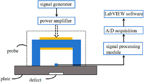
Figure 1. Homemade pulsed alternating current electromagnetic field detection system.

Figure 2

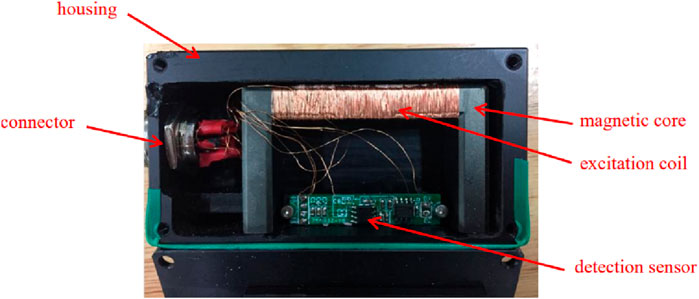
Figure 2. Picture of the probe of the homemade pulsed AC electromagnetic field detection system.

Along with the square wave excitation signal, the typical transient response signal, the induced magnetic field strength versus time curve, of the defects under the pulsed AC electromagnetic field is shown in Figure 3.

Figure 3

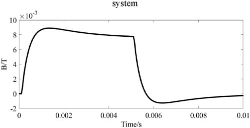
Figure 3. Typical transient response signal of the defect using the pulsed AC electromagnetic field measurement method, induced magnetic field strength versus time plot.

2.2 Customized defect test specimen

The defect test specimen used in this study is an artificially created defect specimen prepared by Shandong Ruixiang Mould Co., Ltd., a professional electrical discharge machining manufacturer, following the customized design shown in Figure 4a. The specimen is made of aluminum panel and has a length of 640 mm, a width of 350 mm, and a thickness of 10 mm. The aluminum panels (electrical conductivity: 35.5 MS/m) were purchased from Shandong Ruixiang Mould Co., Ltd. There are 5 artificial defects distributed on the aluminum specimen, each with a length of 50.0 mm and a width of 0.5 mm. The depths of the five defects, namely, defects 1, 2, 3, 4, and 5 from left to right as shown in Figure 4a, are 9.0 mm, 8.0 mm, 7.0 mm, 6.0 mm, and 5.0 mm, respectively, consistent with the dimensions of the simulation model. Figure 4b shows the picture of the artificial defect specimen. The surface with the defects visible is defined as the front side of the defect specimen, and the other side with a flat aluminum surface is defined as the back side of the defect specimen. From the back side, the defects 1, 2, 3, 4, and 5 are not visible and are the subsurface defects with the buried depths of 1.0 mm, 2.0 mm, 3.0 mm, 4.0 mm, and 5.0 mm, respectively.

Figure 4

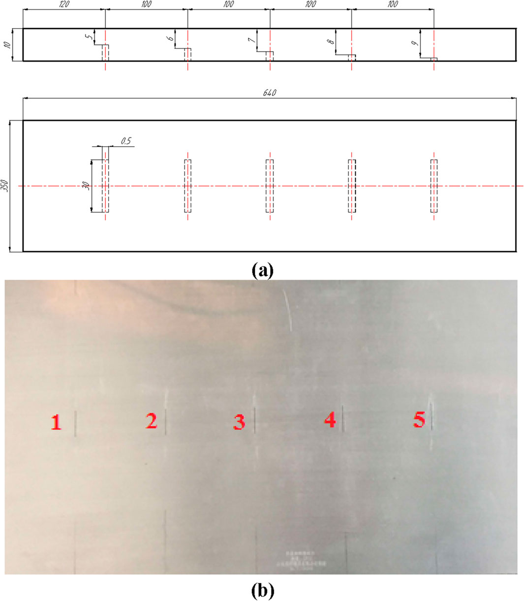
Figure 4. (a) Schematic diagrams of the design of the specimen with artificial defects; (b) Picture of the artificial defect specimen showing five defects, each with a length of 50.0 mm and a width of 0.5 mm. The depths of the five surface defects 1, 2, 3, 4, and 5 are 5.0 mm, 6.0 mm, 7.0 mm, 8.0 mm, and 9.0 mm, respectively.

2.3 Feature extraction from defect signals obtained by pulsed AC electromagnetic fields using principal component analysis

The PCA model was trained by a training sample set to identify and classify various defects. The training data set contains different types of PACFM defect signals, including signals of surface defects with different depths and subsurface defects at different burial depths. The eigensignals of the training samples were obtained by arranging the signals obtained at each given time into a column vector, denoted as Γ_n, with a length N, determined by the number of sampling points. For M measurements, a matrix Γ of dimension M × N was obtained as showned in Equation 1 (Reddy et al., 1997):

$\mathit{\Gamma }=\left[{\mathit{\Gamma }}_1,{\mathit{\Gamma }}_2,{\mathit{\Gamma }}_3,\cdots ,{\mathit{\Gamma }}_M\right](1)$

The key to PCA is to calculate the covariance matrix of the matrix Γ. Directly calculating the covariance matrix of the matrix Γ can be time-consuming and memory-intensive due to its large size. To facilitate the calculation of the covariance matrix, we first centered the data, that is, the mean signal was subtracted from the original signal. The mean signal is defined as shown in Equation 2.

$\overline{\mathit{\Gamma }}=\frac{1}{M}{\displaystyle \sum _{n=1}^M}{\mathit{\Gamma }}_n(2)$

Then, the centered signal is defined as shown in Equation 3.

${\mathrm{\Phi }}_n={\mathit{\Gamma }}_n-\overline{\mathit{\Gamma }}(3)$

The covariance of the centered signal Φ_n is represented by the inner product of vectors, as shown in Equation 4.

$C=\frac{1}{M}{\displaystyle \sum _{n=1}^M}{\mathrm{\Phi }}_n·{{\mathrm{\Phi }}_n}^T=\frac{1}{M}A·A^T(4)$

where C is the covariance matrix of dimension N × N, A = [Φ₁, Φ₂, Φ₃,⋯, Φ_M], and φ^T and A^T are the respective matrix transpose. The direct determination of the eigenvalues and eigenvectors of the covariance matrix C requires a large number of calculations due to its high dimensionality. We calculated the eigenvalues and eigenvectors of the covariance matrix C from another perspective. A^T × A is an M × M matrix, whose dimension is much smaller than that of the covariance matrix C. If v_i and μ_i are the eigenvectors and eigenvalues of the matrix A^T × A, respectively, as shown in Equation 5, then the eigenvectors of the covariance matrix are obtained through Equation 6.

${\mathit{A}}^T\mathit{A}{\nu }_i={\mu }_i{\nu }_i(5)$

${\mu }_i=\mathit{A}{\nu }_i(6)$

Any original signal can be obtained by a linear combination of the eigenvectors μ_i. The eigenvectors are arranged in order of the eigenvalue size, where larger eigenvalues in the original data contain more information. Therefore, the first K largest eigenvalues and their corresponding eigenvectors were taken to form the eigenspace. Thus, for any signal Γ, its representation in the eigenspace is:

$w_k={\mu }_k^T\mathrm{\Gamma }(7)$

where w_k represents the signal’s mapped value into the corresponding eigenvector direction, the coordinates in the eigenspace. These mapped values are the signal features used for defect identification and classification.

The PCA-based defect feature extraction, the calculation and data analysis as well as analysis of the defect response signal were all carried out using the MATLAB software.

2.4 Defect classification and quantification method

Defect classification was performed using the proposed classification algorithm once a defect was identified by PACFM. If the defect was classified as a surface defect, its parameters, such as length, width, and depth, could be quantified using traditional ACFM characteristic features (Gan et al., 2018). If the defect was identified as a subsurface defect, the proposed quantification method was employed to estimate the burial depth. Figure 5 shows the block diagram of defect classification and quantification. The training data set was obtained from artificial defect samples, and principal component analysis was applied to this data set to extract the eigen vectors. The mapped values of the defect signal in the direction of the corresponding eigenvector were calculated and utilized to classify the type of defect and quantify the burial depth of subsurface defects.

Figure 5

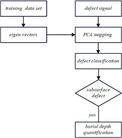
Figure 5. Block diagram of defect classification and quantification using PACFM Combined with PCA.

3 Results and discussion

The front and back sides of the defect specimen shown in Figure 4 were inspected using PACFM for the detection of surface and subsurface defects, respectively. Samples with surface defects with depths of 5.0 mm, 6.0 mm, 8.0 mm, and 9.0 mm on the front side of the defect specimen, and subsurface defects with burial depths of 5.0 mm, 4.0 mm, 2.0 mm, and 1.0 mm on the back side, were selected as defect trial samples for PCA model training. Each defect was detected 8 times using PACFM, with slight variations in the defect’s positioning during each measurement to obtain a sufficiently large amount of defect sample data. A total of 64 defect data sets were obtained.

During each defect measurement, the data from one excitation cycle was collected and arranged into a column vector. With a pulse excitation frequency of 100 Hz and a sampling frequency of 50,000 Hz, the data collected for one excitation cycle included 500 points, allowing for a matrix representation of the sample set used for PCA training.

PCA was used for the time-domain signal data analysis. The eigenvectors of the two largest eigenvalues corresponding to the two principal components were selected as the eigensignals. Figure 6 shows the two eigensignals extracted from the time-domain signals. These two eigensignals contain most of the information contained in the original data.

Figure 6

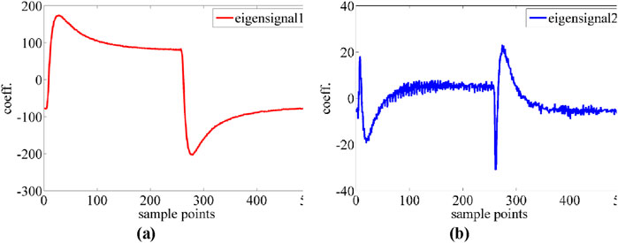
Figure 6. Time domain eigensignals in PCA analysis. Coefficient versus sample points curves for (a) Eigensignal 1 and (b) Eigensignal 2, respectively.

3.1 Defect classification

After the eigensignals were obtained, the defect sample, which was not used as part of the PCA training set, with a depth of 7.0 mm on the defect specimen (as shown in Figure 4b), was inspected on both the front and back sides for the detection of surface defects with a depth of 7.0 mm and subsurface defects with a burial depth of 3.0 mm, respectively. Five different points were inspected at each defect, and the main components of the time-domain signals, w₁ and w₂, were obtained using Equation 7. The results are presented in Table 1, 2. The w₂ versus w₁ plot is shown in Figure 7. The graph shows that subsurface defects are distributed in the first quadrant of the w₂ versus w₁ coordinate system, where w₂ is greater than 0, while surface defects are distributed in the fourth quadrant, where w₂ is less than 0. The results show that defect classification and identification for aluminum samples could be achieved based on the sign of w₂.

Table 1

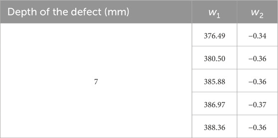
Table 1. Principal component analysis main components w₂ and w₁ of the PACFM signals of the defect with a depth of 7.0 mm.

Table 2

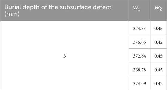
Table 2. Principal component analysis main components w₂ and w₁ of the PACFM signals of the subsurface defect with a burial depth of 3.0 mm.

Figure 7

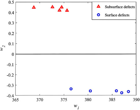
Figure 7. Main component w₂ versus w₁ plot of the principal component analysis of the subsurface defect PACFM signals with the subsurface defect of a burial depth of 3.0 mm.

3.2 Quantitative deduction of the relationship of w₂ and burial depth of defects

The PACFM response signals of subsurface defects with burial depths of 1.0 mm, 2.0 mm, 4.0 mm, and 5.0 mm were quantitatively analyzed using PCA. The corresponding principal component, w₂, for each defect was calculated and is presented in Table 3. A polynomial fit was performed to analyze the relationship between burial depth and w₂ and the 2nd order polynomial equation, shown in Equation 8 was obtained. The coefficient of determination R-squared of the fitting was 0.9729 and the root mean square error was 0.03122, indicating a good fit. The fitting result is illustrated in Figure 8.

$d_{ms}=-0.02351{\omega }_2^2+0.2361{\omega }_2-0.04419(8)$

where d_ms is the burial depth of the defect.

Table 3

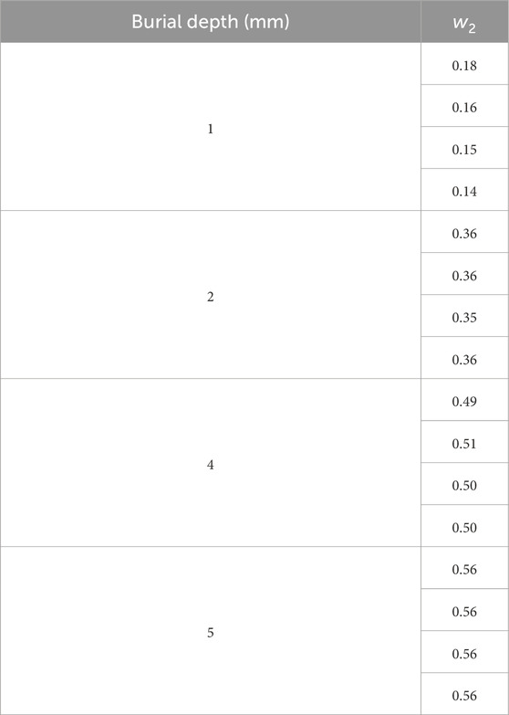
Table 3. Principal components (w₂) of subsurface defect points examined for defects with burial depths of 1.0 mm, 2.0 mm, 4.0 mm, and 5.0 mm; four testing points were examined for each defect using PACFM and PCA analysis.

Figure 8

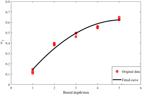
Figure 8. Original data and a polynomial fit of the principal component analysis main component w₂ versus burial depth plot of the subsurface defects with varying burial depths.

3.3 Validation of the defect burial depth quantification algorithm

The principal component w₂ of the subsurface defect with a burial depth of 3.0 mm obtained in Section 3.1 is substituted into the quantification expression of Equation 8 to validate the accuracy of the burial depth quantification algorithm. The results of the calculated burial depth (Table 4) show that the burial depth of subsurface detects can be obtained with high accuracy using the principal component w₂ of the time-domain signal and Equation 8.

Table 4

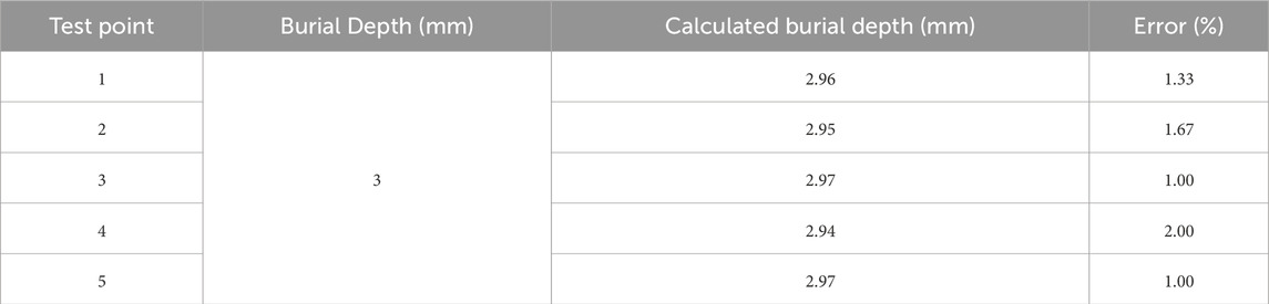
Table 4. Calculated burial depth of the subsurface defect with a burial depth of 3.0 mm using Equation 8 that shows the relationship between the burial depth and the principal component w₂ of the time domain signal.

To further investigate the accuracy of the subsurface defect burial depth quantification algorithm using different defect parameters, we conducted defect detections on a different aluminum specimen with subsurface defects. The length of the defect is 50.0 mm, the width is 2.0 mm, and the depth is 7.0 mm, while the specimen thickness is 10 mm. The defect detection on the specimen from the backside of the specimen was equivalent to detecting subsurface defects with a burial depth of 3.0 mm, and was repeated 5 times with varying defect detecting locations, and the principal component w₂ was calculated for each detection. The results showed that the values of w₂ were all greater than 0, indicating subsurface defects. Substituting w₂ into Equation 8 yields the calculated values of burial depth, as shown in Table 5. The table shows that the calculated burial depth of the subsurface defects has an error averaging around 10% compared to the actual values.

Table 5

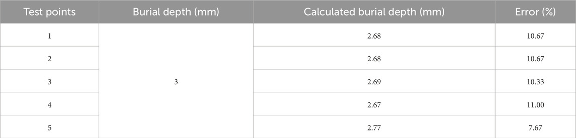
Table 5. Burial depth calculated using the principal component w₂ for subsurface defect detection with a burial depth of 3.0 mm on a different aluminum defect specimen.

4 Conclusion

In this study, we applied principal component analysis to extract specific features from pulsed Alternating Current Field Measurement defect signals for surface and subsurface defect detecting, classification, and quantification for nonferromagnetic materials. The conclusion can be included as follows:

(1) We constructed an artificial defects sample set, including surface defects with depths of 1 mm, 2 mm, 4 mm, and 5 mm, as well as subsurface defects with buried depths of 1 mm, 2 mm, 4 mm, and 5 mm. Eigensignals was obtained by performing principal component analysis on PACFM signals from artificial defects sample set.

(2) The sign of the mapped value w₂ of the defect signal in the corresponding eigenvector direction in the PCA analysis could be used to classify the type of defect. If w₂ is greater than 0, the defect could be identified as subsurface defect, whereas if w₂ is less than 0, the defect could be identified as surface defect.

(3) The magnitude of w₂ could also be used to quantify the burial depth of subsurface defects. We successfully established a quantitative relationship between burial depth and w₂ using a second-order polynomial equation based on the artificial defect sample set. The proposed quantitative algorithm was validated using subsurface defects with different burial depths but the same length and width. The results demonstrated that the proposed algorithm could predict the burial depth of subsurface defects with an error of less than 2%.

(4) The width of subsurface defects might influence the quantification of burial depth. A response signal from defects of different widths in the sample set was used to predict the burial depth using the proposed algorithm, resulting in an average error of approximately 10% compared to the actual values.

In future studies, we will expand the dataset of defect samples to encompass a broader range of defect parameters. This will enable us to better understand and account for the potential impact of these parameters on the quantitative determination of subsurface defect burial depths.

Data availability statement

The original contributions presented in the study are included in the article/supplementary material, further inquiries can be directed to the corresponding author.

Author contributions

QK: Conceptualization, Data curation, Funding acquisition, Investigation, Methodology, Project administration, Software, Writing – original draft, Writing – review and editing. SP: Methodology, Investigation, Writing – review and editing. LL: Investigation, Methodology, Writing – review and editing. XL: Investigation, Methodology, Writing – review and editing.

Funding

The author(s) declare that financial support was received for the research and/or publication of this article. We sincerely appreciate the fundings from: (1) General Research Project of Zhejiang Provincial Department of Education: Development and Application Research of Intelligent Detection System for Pipeline Cracks Based on Alternating Current Electromagnetic Field, Project Number: Y202148134. (2) Major Research Project of Wenzhou Vocational and Technical College: Research and Application of Intelligent Identification Technology for Stress Corrosion Cracks in Valve Welds Based on Alternating Current Electromagnetic Field, Project Number: WZY2021006.

Conflict of interest

The authors declare that the research was conducted in the absence of any commercial or financial relationships that could be construed as a potential conflict of interest.

Generative AI statement

The author(s) declare that no Generative AI was used in the creation of this manuscript.

Publisher’s note

All claims expressed in this article are solely those of the authors and do not necessarily represent those of their affiliated organizations, or those of the publisher, the editors and the reviewers. Any product that may be evaluated in this article, or claim that may be made by its manufacturer, is not guaranteed or endorsed by the publisher.

References

Chen, K., Brennan, F., and Dover, W. (2000). Thin-skin AC field in anisotropic rectangular bar and ACPD stress measurement. Ndt and E Int. 33 (5), 317–323. doi:10.1016/s0963-8695(99)00055-9

CrossRef Full Text | Google Scholar

Cormerais, R., Longo, R., Duclos, A., Wasselynck, G., and Berthiau, G. (2022). Non destructive eddy currents inversion using artificial neural networks and data augmentation. NDT and E Int. 129, 102635. doi:10.1016/j.ndteint.2022.102635

CrossRef Full Text | Google Scholar

Nafiah, F., Tokhi, M. O., Shirkoohi, G., Duan, F., Zhao, Z., Asfis, G., et al. (2020). Parameter analysis of pulsed eddy current sensor using principal component analysis. IEEE Sens. J. 21 (5), 6897–6903. doi:10.1109/JSEN.2020.3036967

CrossRef Full Text | Google Scholar

Feng, Y., Zhang, L., and Zheng, W. (2018). Simulation analysis and experimental study of an alternating current field measurement probe for pipeline inner inspection. Ndt and E Int. 98, 123–129. doi:10.1016/j.ndteint.2018.04.015

CrossRef Full Text | Google Scholar

Gan, F., Li, W., and Liao, J. (2018). New feature for evaluation of subsurface defects via multi-frequency alternating current field signature method. AIP Adv. 8 (1). doi:10.1063/1.5016579

CrossRef Full Text | Google Scholar

Ge, J., Li, W., Chen, G., Yin, X., Liu, J., Kong, Q., et al. (2017). Investigation of optimal time-domain feature for non-surface defect detection through a pulsed alternating current field measurement technique. Meas. Sci. Technol. 29 (1), 015601. doi:10.1088/1361-6501/aa9134

CrossRef Full Text | Google Scholar

Ge, J., Yang, C., Wang, P., and Shi, Y. (2020a). Defect classification based on wavelet packet energy through pulsed alternating current field measurement technique. Electron. Lett. 56 (19), 1016–1019. doi:10.1049/el.2020.1574

CrossRef Full Text | Google Scholar

Ge, J., Yang, C., Wang, P., and Shi, Y. (2020b). Defect classification using postpeak value for pulsed eddy-current technique. Sens. 20 (12), 3390. doi:10.3390/s20123390

PubMed Abstract | CrossRef Full Text | Google Scholar

Greenacre, M., Groenen, P. J., Hastie, T., d’Enza, A. I., Markos, A., and Tuzhilina, E. (2022). Principal component analysis. Nat. Rev. Methods Prim. 2 (1), 100. doi:10.1038/s43586-022-00184-w

CrossRef Full Text | Google Scholar

He, Y., Luo, F., Pan, M., Hu, X., Gao, J., and Liu, B. (2010). Defect classification based on rectangular pulsed eddy current sensor in different directions. Sens. Actuators A Phys. 157 (1), 26–31. doi:10.1016/j.sna.2009.11.012

CrossRef Full Text | Google Scholar

Horan, P., Underhill, P., and Krause, T. (2013). Pulsed eddy current detection of cracks in F/A-18 inner wing spar without wing skin removal using Modified Principal Component Analysis. Ndt and E Int. 55, 21–27. doi:10.1016/j.ndteint.2013.01.004

CrossRef Full Text | Google Scholar

Lewis, A., Michael, D., Lugg, M., and Collins, R. (1988). Thin-skin electromagnetic fields around surface-breaking cracks in metals. J. Appl. Phys. 64 (8), 3777–3784. doi:10.1063/1.341384

CrossRef Full Text | Google Scholar

Li, C., Gao, P., Wang, X., He, B., and Li, J. (2020). “Review on advances in alternating current field measurement testing technology,” in 2020 IEEE far east NDT new technology and application forum (FENDT), 2020. IEEE, 184–188.

CrossRef Full Text | Google Scholar

Mustaqeem, M., and Saqib, M. (2021). Principal component based support vector machine (PC-SVM): a hybrid technique for software defect detection. Clust. Comput. 24 (3), 2581–2595. doi:10.1007/s10586-021-03282-8

PubMed Abstract | CrossRef Full Text | Google Scholar

Nafiah, F., Tokhi, M. O., Shirkoohi, G., Duan, F., Zhao, Z., and Rees-Lloyd, O. (2021). Decoupling the influence of wall thinning and cladding thickness variations in pulsed eddy current using principal component analysis. IEEE Sensors J. 21 (19), 22011–22018. doi:10.1109/jsen.2021.3100648

CrossRef Full Text | Google Scholar

Qiu, X., Zhang, P., Wei, J., Cui, X., Wei, C., and Liu, L. (2013). Defect classification by pulsed eddy current technique in con-casting slabs based on spectrum analysis and wavelet decomposition. Sens. Actuators A Phys. 203, 272–281. doi:10.1016/j.sna.2013.09.004

CrossRef Full Text | Google Scholar

Raine, A., and Lugg, M. (1999). A review of the alternating current field measurement inspection technique. Sens. Rev. 19 (3), 207–213. doi:10.1108/02602289910279166

CrossRef Full Text | Google Scholar

Reddy, V. N., Miller, W. M., and Mavrovouniotis, M. L. (1997). Inverse-signal analysis with PCA. Chemom. Intell. Lab. Syst. 36 (1), 17–30. doi:10.1016/s0169-7439(96)00076-7

CrossRef Full Text | Google Scholar

Sophian, A., Tian, G. Y., Taylor, D., and Rudlin, J. (2003). A feature extraction technique based on principal component analysis for pulsed Eddy current NDT. NDT and e Intern. 36 (1), 37–41. doi:10.1016/s0963-8695(02)00069-5

CrossRef Full Text | Google Scholar

Tamhane, D., Patil, J., Banerjee, S., and Tallur, S. (2021). Feature engineering of time-domain signals based on principal component analysis for rebar corrosion assessment using pulse eddy current. IEEE Sensors J. 21 (19), 22086–22093. doi:10.1109/jsen.2021.3103545

CrossRef Full Text | Google Scholar

Tian, G., Sophian, A., Taylor, D., and Rudlin, J. (2005). Wavelet-based PCA defect classification and quantification for pulsed eddy current NDT. IEE Proc.-Sci. Meas. Technol. 152 (4), 141–148. doi:10.1049/ip-smt:20045011

CrossRef Full Text | Google Scholar

Wei, L., Guoming, C., Wenyan, L., Zhun, L., and Feng, L. (2011). Analysis of the inducing frequency of a U-shaped ACFM system. Ndt and E Int. 44 (3), 324–328. doi:10.1016/j.ndteint.2010.10.009

CrossRef Full Text | Google Scholar

Zhao, J., Li, W., Yin, X., Chen, Q., Zhao, J., Hu, D., et al. (2024). A novel transition frequency for identification and evaluation of subsurface cracks based on alternating current field measurement technique. Meas 231, 114615.

Google Scholar

Zhao, J., Li, W., Yin, X., Li, X., Zhao, J., Fan, M., et al. (2023). Novel phase reversal feature for inspection of cracks using multi-frequency alternating current field measurement technique. Mech. Syst. Signal Pr. 186, 109857. doi:10.1016/j.ymssp.2022.109857

CrossRef Full Text | Google Scholar