Application of clustering algorithms to void recognition by 3D ground penetrating radar

The manual interpretation of ground-penetrating radar images is characterised by long interpretation cycles and high staff requirements. The automated interpretation schemes based on support vector machines, digital images, convolutional neural networks and other techniques proposed in recent years mainly detect features from B-scan slices of 3D ground-penetrating radar data, without taking full advantage of the multi-channel acquisition of data from 3D ground-penetrating radar and joint discrimination. This paper proposes a void recognition algorithm based on cluster analysis algorithm, using VRADI algorithm to process 3D ground-penetrating radar B-Scan, using DBSCAN clustering algorithm to divide clusters and remove noise; proposes correlation weighting coefficient $W_{i,j}$ to quantitatively evaluate the degree of correlation of different survey channels, proposes prime relative position coefficient $P_d$ indicator to quantitatively evaluate the position similarity, and proposes weighted homocentric overlap coefficient ${\mathrm{P}}_{\mathrm{r}}$ indicator to quantify signal similarity. This paper applies the algorithm to carry out physical engineering experiments and uses binary logistic regression analysis to develop a correlation model. The experimental results show that significance of ${\mathrm{P}}_{\mathrm{d}}$ and ${\mathrm{P}}_{\mathrm{r}}$ are less than 0.05, both of which are important influencing indicators for the determination of the presence or absence of void. With an optimal critical probability of 0.4, the recognition accuracy of VRADI algorithm increases from 71.7% to 92.2%. The VRADI algorithm combined with the cluster analysis algorithm outperforms manual recognition in terms of accuracy (92.2% > 83.9%) and recall (90.5% > 86.9%), and the algorithm has good engineering application value.

1 Introduction

Due to backfill or erosion of the roadbed and settlement of the lower structural layer, voids may form within the structural layer. Voids that are not detected and treated in time may develop further and expand under the continuous action of forming conditions, causing pavement subsidence or collapse accidents and threatening traffic safety (LIU et al., 2014; Klotzsche et al., 2019). For roads or areas where there is a risk of voids, it is necessary to carry out voids inspection and detection to provide early warning and treat void damage. Ground Penetrating Radar (GPR) is one of the representative techniques for non-destructive testing of roads, mainly by analysing the propagation of electromagnetic waves within a probe to obtain information about the probe, including information about internal road defects such as voids (Wang et al., 2020).

Three-dimensional ground-penetrating radar uses multiple antennas and has the advantage of full coverage, high accuracy of defect judgement and quantitative analysis of defect compared to two-dimensional ground penetrating radar, which combines multiple sections of data to determine defect (Chen et al., 2017). This paper uses 3D ground penetrating radar images to carry out research work on the automatic recognition of void images. Due to the multi-solution of ground penetrating radar image interpretation, the internal condition of road structure cannot be inferred from the radar image alone, but also needs to be combined with radar theory basis, engineering experience and other related knowledge experience to exclude partial interpretation in order to get the correct interpretation of the radar image (Yu et al., 2020). The long cycle time, low efficiency and high professional requirements of processors in the manual interpretation process currently make radar image interpretation a difficult area for ground-penetrating radar defect detection applications and one of the reasons for limiting the development of ground-penetrating radar applications (Yu et al., 2017).

To solve the problem of automated ground-penetrating radar image interpretation, researchers have proposed numerous radar signal processing algorithms, such as traditional machine learning algorithms, deep learning methods and convolutional neural networks. Traditional machine learning methods use machine vision techniques to detect characteristic hyperbolas in B-SCAN images, with commonly used algorithms including Hough transform-based methods and feature expression-based methods. Hough transform is an effective method for detecting and locating straight lines and resolving curves, but with a large parameter space and high computational complexity. methods for feature representation, such as the Viola-Jones algorithm based on Haar-like wavelet features (Chen et al., 2021); hyperbolic feature detection algorithms combining gradient direction histograms with edge histogram descriptors (Yu et al., 2021). The convolutional neural network method can be used to perform the task of identifying similar features in other unlabelled images by learning correctly labelled images.

Haifeng Li et al. proposed a two-stage recognition method for GPR-RCNN in (Li et al., 2021). The method achieves the recognition of target objects such as voids, pipelines and subsidence with an accuracy of 62%. Pham et al., Lei et al. and Wang Hui et al. all studied the problem of hyperbolic detection in B-SCAN images in different scenes based on faster regional convolutional neural networks (Pham and Lefèvre, 2018), respectively; Zhang et al. (Zhang et al., 2020) investigated the problem of detecting characteristic hyperbolas of water damage targets in asphalt pavements using ResNet50, YOLOV2 network; Zhiyong Huang et al. (Huang et al., 2022) proposed a digital image-based algorithm for radar void signal recognition. The algorithm has advantages in void recognition accuracy and indicator detection, and does not require large amounts of data for training or correction parameters. However, current automatic recognition algorithms of various types mainly detect features from B-scan slices of 3D ground penetrating radar data, without taking full advantage of the multi-channel acquisition of data by 3D ground-penetrating radar and joint discrimination.

The clustering algorithm aggregates n objects into k clusters (k < n) and tries to make the similarity of objects within the same cluster as large as possible. The classical clustering algorithms, depending on the task and the way they are implemented, are the K-Means algorithm, the K-medoids algorithm, the K-modes algorithm, the k-prototypes algorithm, CLARANS, K-Means++, bi-KMeans, etc. There are also K-modes-CGC, K-means-CP and other algorithms that improve on the classical algorithms. Void defect 3D ground-penetrating radar signals are present in multiple B-scans and are similar. The clustering algorithm can be applied to divide voids signals in multiple B-scans of 3D ground penetrating radar into several “clusters”, and then analyse the similarity between the void signals of B-scans in each cluster, and screen out some of the void signals that occur individually or with low similarity, so as to reduce the false alarm rate of 3D ground penetrating radar voids recognition. To this end, this paper investigates a method for detecting void features in 3D ground penetrating radar data that combines an automated B-scan interpretation method and a clustering algorithm.

2 3D ground-penetrating radar void detection and recognition

The 3D ground-penetrating radar used in this paper includes the GEOSCOPE™ MK IV radar host, DXG series multi-channel coupled antenna array, real-time kinematic (RTK), photoelectric encoder, and 3D ground-penetrating radar antenna parameters are shown in Table 1.

TABLE 1

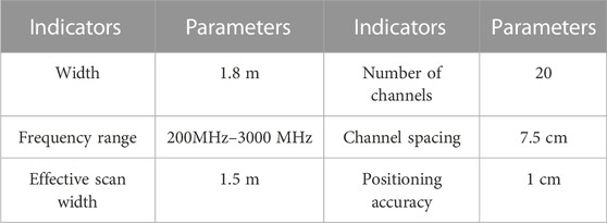
TABLE 1. Technical parameters of the antenna of 3D ground penetrating radar system.

The basic detection principle of 3D ground penetrating radar is to send high-frequency electromagnetic waves in the form of pulses underground, which are reflected when they encounter underground target bodies with electrical differences in the process of propagation in the underground medium (Huai et al., 2019; Allroggen et al., 2020; Domenzain et al., 2020; Tang et al., 2022a). The model of electromagnetic wave propagation and reflection in a medium is shown in Figure 1. The reflection coefficient and reflected signal level can generally be calculated by Eqs 1, 2:

${\mathrm{\Gamma }}_{\mathrm{1,2}}=\frac{\sqrt{{\mathrm{\epsilon }}_{\mathrm{r}1}}-\sqrt{{\mathrm{\epsilon }}_{\mathrm{r}2}}}{\sqrt{{\mathrm{\epsilon }}_{\mathrm{r}1}}+\sqrt{{\mathrm{\epsilon }}_{\mathrm{r}2}}}(1)$

${\mathrm{E}}_{\mathrm{r}1}={\mathrm{E}}_{\mathrm{i}}{\mathrm{\Gamma }}_{\mathrm{1,2}}(2)$

where ${\mathrm{\Gamma }}_{\mathrm{1,2}}$ is the interfacial reflection coefficient, ${\mathrm{\epsilon }}_{\mathrm{r}1}$ is the relative dielectric constant on the incident side of electromagnetic waves, ${\mathrm{\epsilon }}_{\mathrm{r}2}$ is the relative dielectric constant on the outgoing side of electromagnetic waves, ${\mathrm{E}}_{\mathrm{r}1}$ is the reflected signal level and ${\mathrm{E}}_{\mathrm{i}}$ is the incident signal level. As can be seen from the equation, the positive and negative reflection coefficients and their magnitude are determined by the magnitude of relative dielectric constants of the substances on either side of the void interface. The greater the difference in relative dielectric constants between the two sides of the interface, the greater the reflection coefficient and the stronger the reflected signal.

FIGURE 1

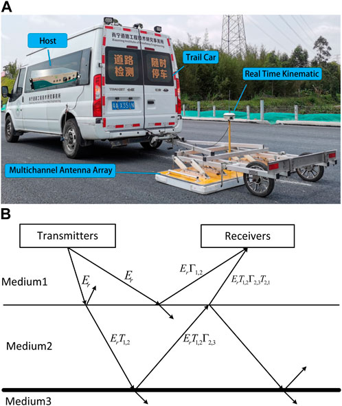
FIGURE 1. Ground penetrating radar system and electromagnetic wave propagation model: (A) 3D ground penetrating radar system components (B) Ground penetrating radar electromagnetic wave propagation models in different media.

There is a significant difference in the relative dielectric constants of the void fill and the road construction material. The interior of the void is generally air with a relative dielectric constant of 1. Road materials generally have a relative dielectric constant between 3 and 10. Electromagnetic waves emitted by 3D ground penetrating radar are reflected at the void-road material interface (FIROOZABADI et al., 2007; Leng and Al-Qadi, 2014; Kumlu, 2021; Tang et al., 2022b). After the ground-penetrating radar receives the reflected electromagnetic wave signal, according to the signal propagation time and amplitude, it is recorded and stored as 3D ground penetrating radar data, and Examiner software is used to filter the data, the parameters are set as shown in the Figure 2, and the radar grey-scale image is drawn, as shown in the Figure 3.

FIGURE 2

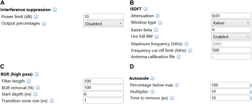
FIGURE 2. Examiner software filtering settings: (A) Interference suppression; (B) ISDFT; (C) BGR (high pass); (D) Autoscale.

FIGURE 3

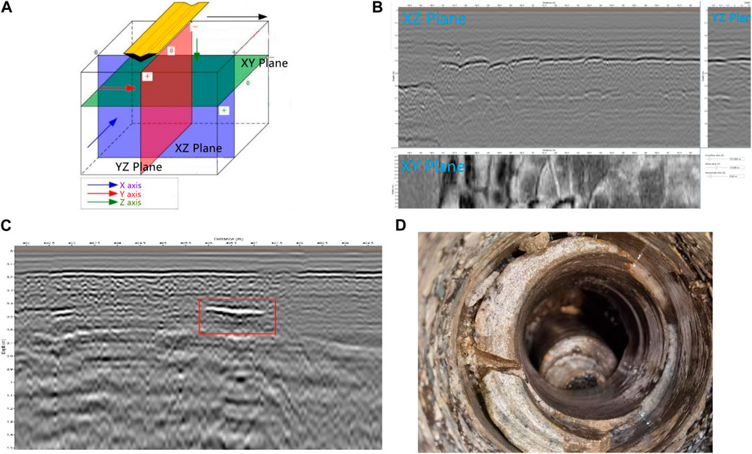
FIGURE 3. 3D ground penetrating radar data slices, void feature signals and drill core verification results: (A) Three types of slicing of 3D ground-penetrating radar data; (B) Schematic diagram of XY section, YX section and XZ section; (C) YX-section void feature signal (D) Validation of void defects boreholes.

Please refer to the paper (Jacopo and Neil, 2012; Tang, 2020) for a detailed explanation of parameter settings and numerical settings. “Interference suppression” is a frequency domain filtering tool used to eliminate interference from external radio transmitters, such as mobile phone base stations. The echo intensity of the DXG 1820 is generally not greater than 10dB, so setting 10 dB removes electromagnetic wave signals greater than this value. The function of “ISDFT” filtering processing is to convert frequency domain data into time domain data. “Attenuation” represents the absoption in the material and controls the shape of the high freqeuncy cut-off for deep data. Higher values will remove more of the higher fregeuncies. The recommended value is 0.01. “Use full BW” enables to use the full recorded bandwidth, while the frequency bandwidth of the DXG1820 is 500–3000 MHz.

“BGR (high pass)” is a time-domain filtering tool that utilizes high pass filtering to remove background, mainly horizontal echo signals, in a certain proportion. Generally speaking, the loss of electromagnetic waves is exponentially related to the propagation time. “Autoscale” calculates the gain coefficient based on the attenuation law of radar signals, compensates for the attenuation multiple of deep echo signals, and makes the overall intensity of the ground penetrating radar image signal uniform.

Manual recognition of the void signal is mainly done by intercepting the XZ section in the 3D ground-penetrating radar data. If the void cavity is filled with air, the radar reflection signature signal is a higher intensity homophase axial signal with black on both sides (side flaps) and white in the middle (main flaps) (CAPINERI et al., 1998; SOLLA et al., 2014; CHA et al., 2017; Maeda et al., 2018; Liu et al., 2021), as shown in Figure 3C, and the corresponding borehole verification results for this location are shown in Figure 3D.

3 Principles of clustering analysis algorithms for 3D ground-penetrating radar data

3D ground penetrating radar is an effective means of detecting void, but at present, whether by manual recognition or automatic recognition algorithms, 3D ground-penetrating radar detection of void signals cannot be completely accurate due to the multi-solution of ground-penetrating radar image interpretation. Taking advantage of the multi-channel acquisition of data by 3D ground-penetrating radar, a clustering analysis algorithm is used to improve the accuracy of recognition.

3D ground-penetrating radar antenna has 20 channels and the lateral spacing between adjacent channels is 0.075m, due to the fact that the width of the voiding area is generally greater than 0.075 m and the reflected electromagnetic wave signal has a scattering effect. As a result, the voiding signals will appear in several B-scans at the same time, and since the detection targets are the same and the electromagnetic wave propagation paths in different channels are basically the same, the degaussing signals appearing in adjacent channels will often be in close proximity and have a high degree of similarity.

Projection of 3D ground penetrating radar void signal onto the same plane, based on the distance between the projected positions and the similarity of the areas, can further determine the confidence of whether the detected signal is a void signal. Projected void radar signals with distant locations and low regional similarity imply a low confidence level, as shown in the figure. The projected void radar signals that are located close together and have a high degree of regional similarity imply a high confidence level, as shown in Figure 4.

FIGURE 4

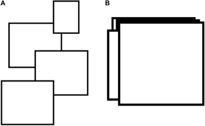
FIGURE 4. Two cases of overlapping areas of adjacent channel B scanning: (A) Projected positions spaced far apart and with low regional similarity; (B) Projected positions relatively close to each other and with a high degree of regional similarity.

The main purpose of applying clustering algorithm is to quantitatively describe positional similarity and signal similarity between the suspected voiding signals detected by the different survey channels, the higher the degree, the higher the probability of determining the point as a void defect. The steps of clustering analysis algorithm for ground-penetrating radar data void signals method are shown in the following Figure 5 and can be divided into the following steps:

FIGURE 5

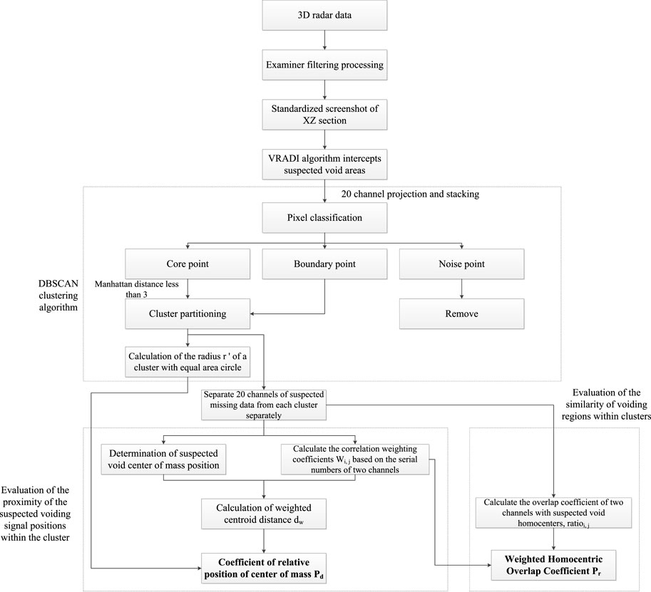
FIGURE 5. Data processing flowchart of 3D ground penetrating radar data clustering analysis algorithm.

1) Data preparation: Standardisation of 3D ground penetration data. Examiner software is used to filter the data and intercept its XZ cross-sections, the resolution of cross-sections, the colouring method should be consistent. The resolution of the images in this study is 350 × 300 and the colouring method is grey-scale colouring, as shown in Figures 6A–D for the radar images of channels 8 to 11 of XZ section void radar data with the same Y-axis range and different channels.

2) Feature extraction: The Void recognition algorithm based on the digital image (VRADI) algorithm proposed in the paper (Huang et al., 2022) is applied to process the radar image database and output the binarised image recognition results to determine the suspected voiding signal. Suspected voiding pixels are assigned a value of 1 and non-suspected voiding pixels are assigned a value of 0. The results of radar image processing for channels 8 to 11 are shown in Figures 6E–H).

3) Clusters dividing: In real space, regions that are connected to each other belong to the same void. In B-scan slices, regions with a high density of suspected voiding pixels are connected to each other, the higher the probability of belonging to the same void. To describe this relationship quantitatively, the binarised images of all channels are projected onto the same plane and accumulated to obtain a superimposed plane $P_1$, where the pixel values of the superimposed plane are equal to the accumulated values of the multi-channel XZ section recognition results, and the processing results are shown in Figure 6I. Applying DBSCAN (Zou et al., 2021) clustering algorithm to the superimposed planes, the algorithm steps are:

FIGURE 6

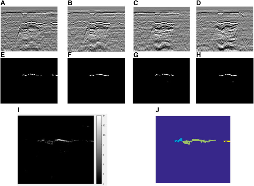
FIGURE 6. Example data preparation, feature extraction and clusters dividing: (A) Channel 8 B-Scan; (B)Channel 9 B-Scan; (C)Channel 10 B-Scan; (D)Channel 11 B-Scan; (E) Channel 8 VRADI; (F)Channel 9 VRADI processing results; (G)Channel 10 VRADI processing results; (H)Channel 11 VRADI processing results; (I) Superimposed plane $P_1$ for all channel VRADI processing results; (J) DBSCAN clustering algorithm divides the processing results into three clusters (indicated by different colours).

1. The suspected voiding pixels are classified as core points, boundary points, and noise points. The principle of division is: the distance metric uses the Manhattan distance, taking point A as the centre and calculating the sum of all pixel values less than or equal to 3. If the sum is greater than or equal to 25 (the number of pixel points), the point is judged to be the core point, and other pixel points with values greater than 0 are the boundary points. The points that are neither core nor boundary points are classified as noise points. And so on, going through all the pixel points.

${\mathrm{d}}_{\mathrm{i},\mathrm{j}}=\left|{\mathrm{x}}_{\mathrm{i}}-{\mathrm{x}}_{\mathrm{j}}\right|-\left|{\mathrm{y}}_{\mathrm{i}}-{\mathrm{y}}_{\mathrm{j}}\right|(3)$

where, ${\mathrm{d}}_{\mathrm{i},\mathrm{j}}$ is Manhattan distance between two pixel points, ${\mathrm{x}}_{\mathrm{i}}$, ${\mathrm{x}}_{\mathrm{j}}$ are the X-axis coordinates of pixel points i,j, and ${\mathrm{y}}_{\mathrm{i}}$, ${\mathrm{y}}_{\mathrm{j}}$ are the Y-axis coordinates of pixel points i,j.

As shown in Figure 7, with (6,4) and (7,5) as the centers, the sum of pixel values with a Manhattan distance less than 3 is 43 and 29, respectively. Therefore, these two points are both core points. The sum of pixel values centered on (4,9) (marked in yellow) is less than 25, but within the range (6,4) and (7,5) are all core points, so (4,9) is the boundary point.

FIGURE 7

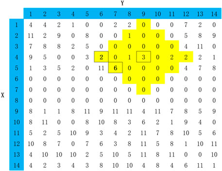
FIGURE 7. Calculation principle for dividing center points, boundary points, and noise points.

2. Any two Manhattan core points with a distance less than or equal to 3 are grouped into the same cluster, and any boundary points within a radius of 3 of the core points are placed in the same cluster as the core points. The noise points are removed, the core points and boundary points are retained, the suspected voiding signal region is updated, and the suspected voiding signals are clustered into several clusters.

3. Calculate the superimposed plane area of each cluster Area, the superimposed plane area is equal to the number of pixels greater than 0; and calculate the equal area circle radius ${\mathrm{r}}^{\prime }$ , the equal area effect circle calculation formula is shown in Eq. 4.

$r^{\prime }=\sqrt{\frac{Area}{\pi }}(4)$

where, Area is the area of the superimposed plane of the cluster; $\mathrm{\pi }$ is the circumference; ${\mathrm{r}}^{\prime }$ is the radius of the equal area circle.

4) Evaluation of the proximity of the suspected voiding signal positions within the cluster.

1. The centroid of the suspected voiding signal is used to represent the position of the signal, and the coordinates of the centroid are calculated as shown in Eq. 5; at the same time, the distance between the two centroids of the suspected voiding signal within the cluster is calculated, and the Euclidean distance is used for the two-point distance metric, calculated as shown in Eq. 6.

${\mathrm{x}}_{\mathrm{c}},{\mathrm{y}}_{\mathrm{c}}=\left(\frac{{\displaystyle \sum _{\mathrm{j}=1}^{\mathrm{n}}}{\mathrm{x}}_{\mathrm{j}}}{\mathrm{n}},\frac{{\displaystyle \sum _{\mathrm{j}=1}^{\mathrm{n}}}{\mathrm{y}}_{\mathrm{j}}}{\mathrm{n}}\right)(5)$

where ${\mathrm{x}}_{\mathrm{i}}$, ${\mathrm{y}}_{\mathrm{i}}$ are the x- and y-axis coordinates of the centroid, n is the number of pixels in the suspected voiding region, ${\mathrm{x}}_{\mathrm{j}}$, ${\mathrm{y}}_{\mathrm{j}}$ are the x- and y-axis coordinates of the $j$ pixel in the suspected voiding region.

${\mathrm{d}}_{\mathrm{i},\mathrm{j}}^{\prime }=\sqrt{{\left({\mathrm{x}}_{\mathrm{i}}-{\mathrm{x}}_{\mathrm{j}}\right)}^2+{\left({\mathrm{y}}_{\mathrm{i}}-{\mathrm{y}}_{\mathrm{j}}\right)}^2}(6)$

where, ${\mathrm{d}}_{\mathrm{i},\mathrm{j}}^{\prime }$ is the Euclidean distance between centroids i,j, $x_i$, ${\mathrm{x}}_{\mathrm{j}}$ are the x-axis coordinates of centroids i,j, and ${\mathrm{y}}_{\mathrm{i}}$, ${\mathrm{y}}_{\mathrm{j}}$ are the y-axis coordinates of centroids i,j.

${\mathrm{W}}_{\mathrm{i},\mathrm{j}}=\frac{1}{\left(\mathrm{j}-\mathrm{i}\right){\displaystyle \sum _{\mathrm{j}=1}^{\mathrm{m}-1}}{\displaystyle \sum _{\mathrm{j}=\mathrm{i}+1}^{\mathrm{m}}}\frac{1}{\left(\mathrm{j}-\mathrm{i}\right)}}\mathrm{i},\mathrm{j}\in \left[1,\mathrm{m}-1\right],\mathrm{i}<\mathrm{j}(7)$

where, ${\mathrm{W}}_{\mathrm{i},\mathrm{j}}$ is the correlation weighting factor between channels i,j; m is the total number of channels in the cluster where there is a suspected voiding region, and channels where there is no suspected deglomeration region in the cluster are not involved in the calculation. A larger ${\mathrm{W}}_{\mathrm{i},\mathrm{j}}$ represents a stronger correlation between the suspected voiding areas of the two channels.

3. Combining the weighting factors and the centroid distance, the overall weighted centroid distance ${\mathrm{d}}_{\mathrm{w}}$ between the suspected voiding signals within the cluster is calculated according to Eq. (8).

${\mathrm{d}}_{\mathrm{w}}={\displaystyle \sum _{\mathrm{j}=1}^{\mathrm{m}-1}}{\displaystyle \sum _{\mathrm{j}=\mathrm{i}+1}^{\mathrm{m}}}{\mathrm{W}}_{\mathrm{i},\mathrm{j}}*{\mathrm{d}}_{\mathrm{i},\mathrm{j}}^{\prime }\mathrm{i},\mathrm{j}\in \left[1,\mathrm{m}-1\right],\mathrm{i}<\mathrm{j}(8)$

where, ${\mathrm{d}}_{\mathrm{w}}$ is the overall weighted centroid distance between suspected voiding signals within a cluster; ${\mathrm{W}}_{\mathrm{i},\mathrm{j}}$ is the correlation weighting factor between channels i,j; and $d_{i,j}^{\prime }$ is the Euclidean distance between i,j centroid points.

4. Based on the ratio of the weighted centroid distance to the cluster equivalent radius, the relative position coefficient of the centroid is calculated according to Eq. 9.

${\mathrm{P}}_{\mathrm{d}}=\frac{{\mathrm{d}}_{\mathrm{w}}}{{\mathrm{r}}^{\prime }}(9)$

where, ${\mathrm{d}}_{\mathrm{w}}$ is the weighted centroid distance between the suspected voiding signals within the cluster; ${\mathrm{r}}^{\prime }$ is the radius of the equal area circle. A larger ${\mathrm{P}}_{\mathrm{d}}$ represents a higher degree of similarity in position between the suspected voiding regions within the cluster as a whole.

5) Evaluation of the similarity of voiding regions within clusters.

1. The suspected voiding regions of the same cluster are translated to the same location and projected onto the same plane two by two to calculate the homocentric overlap coefficient, which is calculated according to Eq. 10, and the homocentric overlap coefficient represents the signal similarity between the two;

${\text{ratio}}_{\mathrm{i},\mathrm{j}}=\frac{\cup \left({\mathrm{A}}_{\mathrm{i}},{\mathrm{A}}_{\mathrm{j}}\right)}{\cap \left({\mathrm{A}}_{\mathrm{i}},{\mathrm{A}}_{\mathrm{j}}\right)}\mathrm{i},\mathrm{j}\in \left[1,\mathrm{m}-1\right],\mathrm{i}<\mathrm{j}(10)$

where, ${\text{ratio}}_{\mathrm{i},\mathrm{j}}$ is the coefficient of homocentric overlap of the two suspected voiding regions ${\mathrm{A}}_{\mathrm{i}}$, ${\mathrm{A}}_{\mathrm{j}}$ in the cluster; $\cap \left({\mathrm{A}}_{\mathrm{i}},{\mathrm{A}}_{\mathrm{j}}\right)$ is the area of the overlap of the two suspected voiding regions ${\mathrm{A}}_{\mathrm{i}}$, ${\mathrm{A}}_{\mathrm{j}}$ after projection; $\cup \left({\mathrm{A}}_{\mathrm{i}},{\mathrm{A}}_{\mathrm{j}}\right)$ is the total area of the two suspected voiding projections ${\mathrm{A}}_{\mathrm{i}}$, ${\mathrm{A}}_{\mathrm{j}}$; m is the total number of channels in the cluster with suspected voiding areas; larger ${\text{ratio}}_{\mathrm{i},\mathrm{j}}$ means that the suspected voiding areas of the two channels are more similar.

2. It is also necessary to consider the correlation weighting factor $W_{i,j}$ between two suspected voiding signals, calculated according to Eq. 11. Combining the weighting and overlap coefficients, the overall weighted homocentric overlap coefficient ${\mathrm{P}}_{\mathrm{r}}$ between suspected voiding regions within the cluster is calculated.

${\mathrm{P}}_{\mathrm{r}}={\displaystyle \sum _{\mathrm{j}=1}^{\mathrm{m}-1}}{\displaystyle \sum _{\mathrm{j}=\mathrm{i}+1}^{\mathrm{m}}}{\mathrm{W}}_{\mathrm{i},\mathrm{j}}*{\text{ratio}}_{\mathrm{i},\mathrm{j}}\mathrm{i},\mathrm{j}\in \left[1,\mathrm{m}-1\right],\mathrm{i}<\mathrm{j}(11)$

where, ${\mathrm{P}}_{\mathrm{r}}$ is the overall weighted homocentric overlap coefficient between the suspected voiding signals within the cluster; $W_{i,j}$ is the correlation weighting coefficient between channels i,j; ${ratio}_{i,j}$ is the homocentric overlap coefficient of two suspected voiding regions ${\mathrm{A}}_{\mathrm{i}}$, ${\mathrm{A}}_{\mathrm{j}}$ in the cluster. A larger ${\mathrm{P}}_{\mathrm{r}}$ means a higher overall similarity between the suspected voiding regions within the cluster.

The example data shown in Figure 6 is divided into three clusters of suspected voiding signals, with relative position coefficients of 0.7348, 2.5792 and 0.5408 for centroids and weighted homocentric overlap coefficients of 0.012, 0.086 and 0.464.

4 Experiments and analysis of results

4.1 Experimental results

This study relies on road voiding detection in a city in southern China and uses 3D ground penetrating radar scanning to detect urban roads. 3D ground-penetrating radar acquisition parameters are set: sampling spacing (3 cm), time window (100 ns) and standing wave time (1 ms). The road structure combination is 10 cm asphalt concrete pavement +28 cm cement concrete structure +36 cm cement stabilized graded crushed stone + soil foundation, and the inspection is carried out in a full-coverage manner, with a total inspection length of 124 km by measuring line, as shown in Figures 8A–D. The analysis of 3D ground-penetrating radar image by manual recognition and interpretation yielded 87 void defects and the analysis of 3D ground-penetrating radar image by VRADI algorithm yielded 106 void defects, of which 78 void defects obtained by manual recognition and interpretation by VRADI algorithm were void defects in the same location, giving a total of 115 void defects.

FIGURE 8

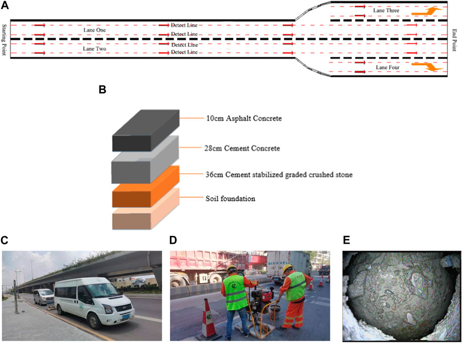
FIGURE 8. Detection plan, pavement structure composition, and void verification. (A) 3D ground-penetrating radar survey line layout diagram. (B) Composition and thickness of pavement structure. (C) Field test inspection chart. (D) Borehole verification test results. (E) Image in void verification hole.

Borehole verification work was carried out on the 115 void detection results, recording parameters such as the presence of void, height and area of void, and collecting images of the interior of defects. As shown in Figures 8D, E, the validation results show that there are a total of 84 void defects and the remaining 31 are false positives. The recall and accuracy rates of the two methods, manual recognition and VRADI algorithm, are calculated based on void validation results, and the formulae are shown in Eqs 12–14.

$\mathrm{Pr}=\frac{TP}{TP+FP}(12)$

$\text{Re}=\frac{TP}{TP+FN}(13)$

$F1-measure=2\times \frac{Precison\times Recall}{Precison+Recall}(14)$

where, TP (True Positive) is the result of deciphering void defect and borehole results are also the result of void defect; FP (False Positive) is the result of deciphering void defect and borehole results are the result of non-void defect; FN (False Negative) is the result of deciphering a non-void defect and borehole for a void defect; Pr (Precision) is the accuracy of the deciphering result; Re (Recall) is the recall of the deciphering result. F1-measure is a comprehensive indicator that reflects the recall and precision.

Combining the validation results, the statistics of the manual recognition interpretation and the VRADI algorithm interpretation analysis are shown in Figure 9A. Of the 84 void defects, the manual recognition of void defect recall was 86.9% and accuracy 83.9%, while the VRADI recall of void defect was 90.5% and accuracy 71.7%.

FIGURE 9

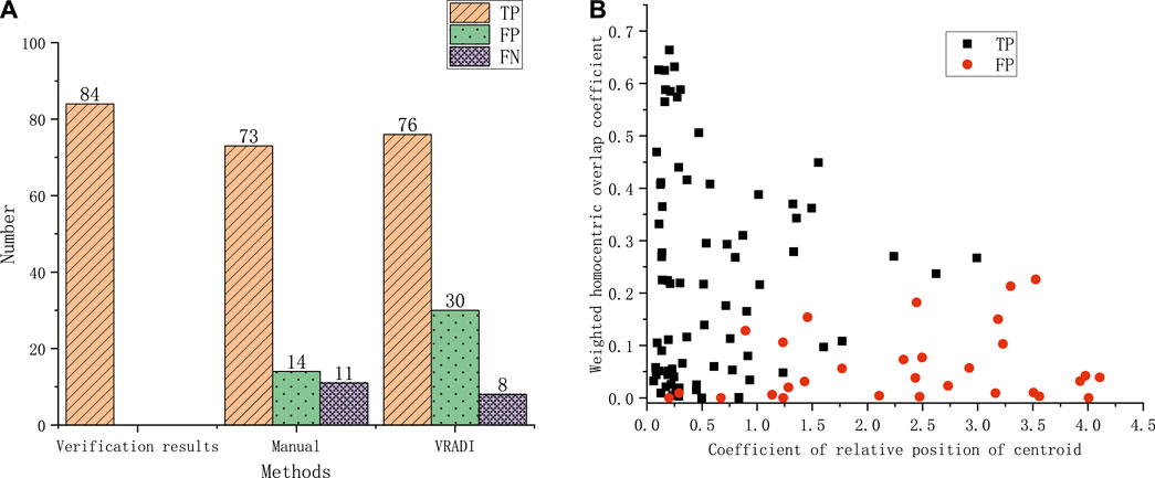
FIGURE 9. Statistical analysis of void recognition results. (A) Statistics of manual recognition and VRADI recognition results. (B) VRADI recognition results and cluster analysis indicator distribution.

For the 106 void defects identified by VRADI algorithm, the radar image data sets were further analysed using 3D ground-penetrating radar data clustering analysis algorithm to calculate the relative position coefficient of each void core and the weighted homocentric overlap coefficient. The results of the borehole verification were combined with the relative position coefficients of the cores and the weighted homocentric overlap coefficients as X and Y-axes, and different colours were used to distinguish the verification results from both voiding and non-voiding defects, and a scatter plot was drawn as shown in Figure 9B.

4.2 Cluster analysis metrics and voiding correlation analysis

Before analysis, the results of the voiding determination are standardised and the presence or absence of voiding is recorded as “0"(no) or “1"(yes), and the relative position coefficients of the centroids and the weighted homocentric overlap coefficients are expressed numerically. SPSS 26 statistical software was used to analyse the data, and binary logistic regression analysis was used to establish the correlation model between the relative position coefficient of the centroids (independent variable), the weighted homocentric overlap coefficient (independent variable) and the outcome of void determination (dependent variable), and the PV critical line of the prediction probability was divided by 0.5, greater than or equal to 0.5, the outcome of the determination was “1"(yes) and less than 0.5, the predicted outcome is “0"(no). The Exp confidence interval was 95% and the model was terminated after eight rounds of fitting with essentially constant parameters. The fitted formula is shown in Eq 15 and the regression result parameters are shown in Table 2.

$P\left(V\right)=\frac{e^{-2.961P_d+24.743P_r+2.319}}{1+e^{-2.961P_d+24.743P_r+2.319}}(15)$

TABLE 2

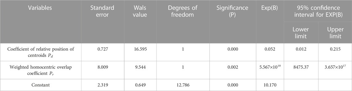
TABLE 2. Parameters of binary logistic regression analysis results.

The results of the analysis showed that the model was able to correctly classify 89.6% of the study subjects, with a prediction accuracy of 80% for “No” and 93.4% for “Yes”. Of the 2 independent variables included in the model, the relative position coefficient ${\mathrm{P}}_{\mathrm{d}}$ (OR = 0.052, OR 95% confidence interval 0.012 to 0.215, p = 0.000) and the weighted homocentric overlap coefficient ${\mathrm{P}}_{\mathrm{r}}$ (OR = 5.567×10^10, OR, 95% confidence interval 8475.37 to 3.657×10¹⁷, p = 0.002). The p-values were all less than 0.05, which was statistically significant and a significant influence in determining the presence or absence of void.

By using Eq. 15 to predict the void determination results, the number of void false positives was reduced from 30 to 6, but the number of accurately predicted void by VRADI was reduced from 76 to 71, the recognition accuracy was increased from 71.7% to 92.2%, and the recognition recall rate was reduced from 90.5% to 84.5%. As missing voids are not expected in practical engineering, the number of missed voids and the number of voids misclassified were fitted to obtain the predicted results at an interval of 0.05 in order to avoid a drop in recall, by adjusting the critical probability as shown in Figure 10.

FIGURE 10

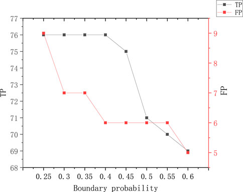
FIGURE 10. Folding graph of TP and FP with probability of partition.

As can be seen from Figure 10, at a critical probability of 0.4, TP is not reduced and FP decreases from 30 to 6, a reduction of 80%. Further increasing the decomposition probability leads to a decrease in TP and decreasing this critical probability leads to an increase in FP, so a critical probability of 0.4 is the optimal value. With this critical probability, the recognition precision of VRADI algorithm improved from 71.7% to 92.2%, the recognition recall remained at 90.5% and the F1-measure increased from 80.0% to 91.3%. The VRADI algorithm combined with the cluster analysis algorithm outperformed the manual recognition in terms of both void recognition precision (92.2% > 83.9%) and recall rate (90.5% > 86.9%).

4.3 Model comparison

We compare our algorithm with three existing methods, including.

Faster R-CNN (Wang et al., 2019). Faster R-CNN is a state-of-the-art two-stage object detection networks depending on region proposal algorithms to hypothesize object locations.

YOLO v7 (Ren et al., 2017)^. You only look once (YOLO) is a state-of the-art, real-time one-stage object detection method.

PIXOR (Wang et al., 2022)^. PIXOR (ORiented 3D object detection from PIXel-wise neural network predictions) is a state-of-theart, real-time 3D Object detection from point clouds in the fifield of autonomous driving.

YOLO and Faster R-CNN represents state-of-the-art one stage and two-stage object detection networks, respectively, but they all belong to 2D object detection networks. PIXOR utilizes the 3D data more effificiently by representing the scene from the Bird’s Eye View. We used the same dataset for training and recognition, and the results are shown in the Table 3.

TABLE 3

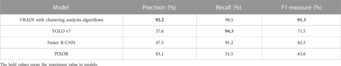
TABLE 3. Parameters of binary logistic regression analysis results.

It can be seen from the Table 3 that the precision and F1-measure of the method used in this paper are higher than other models, and recall is slightly lower than Yolo v7 model and Faster R-CNN model, which is significantly higher than other models. In practical engineering, high accuracy means that the error rate of engineering verification and repair is low, which can reduce unnecessary work. The recognition recall rate of VRADI algorithm is slightly lower than that of Yolo V7, but the difference is small, reaching more than 90%, at the same level, meeting the needs of practical engineering. In terms of F1-measure index which comprehensively reflects the performance of the model, VRADI algorithm is obviously superior to other models, indicating that the comprehensive performance of VRADI algorithm is superior to other models, especially in recognition precision.

5 Conclusion

In this paper, a 3D ground-penetrating radar void defect recognition model based on cluster analysis algorithm is proposed, and the experimental conclusions of the model are as follows.

1. The clustering analysis algorithm of 3D ground-penetrating radar data is based on the feature that the voiding signals appearing in adjacent channels tend to be similar in position and have a high degree of similarity. The relative position coefficient ${\mathrm{P}}_{\mathrm{d}}$ indicator is proposed to quantitatively evaluate the position proximity, the weighted homocentric overlap coefficient ${\mathrm{P}}_{\mathrm{r}}$ indicator is proposed to quantitatively evaluate the signal similarity, and the correlation weighted coefficient ${\mathrm{W}}_{\mathrm{i},\mathrm{j}}$ is proposed to quantitatively evaluate the degree of correlation of different channels;

2. Binary logistic regression analysis was used to develop a correlation model between the relative position coefficient of the centroid (independent variable), the weighted homocentric overlap coefficient (independent variable) and the outcome of the void determination (dependent variable). The results of the model experiments show that the relative position coefficient of the centroid ${\mathrm{P}}_{\mathrm{d}}$ (P = 0.000) and the weighted homocentric overlap coefficient ${\mathrm{P}}_{\mathrm{r}}$ (P = 0.002) are both significant (P) less than 0.05, indicating that both ${\mathrm{P}}_{\mathrm{d}}$, ${\mathrm{P}}_{\mathrm{r}}$ are important influencing indicators for the determination of the existence of voiding, and the regression fitting formula is shown in Eq. 15.

3. To address the problem of decreasing recall rate of recognition using a critical probability of 0.5 for predicting the results of voiding, the critical probability in the binary logistic regression analysis model was adjusted at an interval of 0.05 to obtain the optimal critical probability of 0.4. With this critical probability, the recognition accuracy of the VRADI algorithm improved from 71.7% to 92.2%, and the recognition recall remained at 90.5%. The VRADI algorithm combined with the cluster analysis algorithm outperformed manual recognition in terms of recognition accuracy (92.2% > 83.9%) and recall (90.5% > 86.9%), and has good engineering application value.

4. Compared with three existing methods including YOLO, Faster R-CNN and PIXOR, the precision and F1-measure of the VRADI algorithm used in this paper are higher than other models, indicating that the comprehensive performance of VRADI algorithm is superior to other models, especially in recognition precision.

Data availability statement

The original contributions presented in the study are included in the article/Supplementary material, further inquiries can be directed to the corresponding author.

Author contributions

NZ contributed to conception and design of the study. JT organized the database and performed the statistical analysis and wrote the first draft of the manuscript. NZ, JT, ZH, LW, and ZX wrote sections of the manuscript. All authors contributed to the article and approved the submitted version.

Conflict of interest

Author NZ was employed by the Guangzhou Beihuan Intelligent Transportation Technology Co., Ltd.

The remaining authors declare that the research was conducted in the absence of any commercial or financial relationships that could be construed as a potential conflict of interest.

Publisher’s note

All claims expressed in this article are solely those of the authors and do not necessarily represent those of their affiliated organizations, or those of the publisher, the editors and the reviewers. Any product that may be evaluated in this article, or claim that may be made by its manufacturer, is not guaranteed or endorsed by the publisher.

References

Allroggen, N., Beiter, D., and Tronicke, J. (2020). Ground-penetrating radar monitoring of fast subsurface processes. Geophysics 85, A19–A23. doi:10.1190/GEO2019-0737.1

CrossRef Full Text | Google Scholar

Capineri, L., Grande, P., and Temple, J. A. G. (1998). Advanced image-processing technique for real-time interpretation of ground-penetrating radar images. Int. J. Imaging Syst. Technol. 9 (1), 51–59. doi:10.1002/(sici)1098-1098(1998)9:1<51::aid-ima7>3.0.co;2-q

CrossRef Full Text | Google Scholar

Cha, Y. J., Choi, W., and Buyukozturk, O. (2017). Deep learning-based crack damage detection using convolutional neural networks. Computer-Aided Civ. Infrastructure Eng. 32 (5), 361–378. doi:10.1111/mice.12263

CrossRef Full Text | Google Scholar

Chen, B., Xiong, C., Li, W., He, J., and Zhang, X. (2021). Assessing surface texture features of asphalt pavement based on three-dimensional laser scanning Technology. Buildings 11, 623. doi:10.3390/buildings11120623

CrossRef Full Text | Google Scholar

Chen, B., Zhang, X., Yu, J., and Wang, Y. (2017). Impact of contact stress distribution on skid resistance of asphalt pavements. Constr. Build. Mater. 133, 330–339. doi:10.1016/j.conbuildmat.2016.12.078

CrossRef Full Text | Google Scholar

Domenzain, D., Bradford, J., and Mead, J. (2020). Joint inversion of full-waveform ground-penetrating radar and electrical resistivity data — Part 2: enhancing low frequencies with the envelope transform and cross gradients. Geophysics 85 (6), H115–H132. doi:10.1190/geo2019-0755.1

CrossRef Full Text | Google Scholar

Firoozabadi, R., Miller, E. L., Rappaport, C. M., and Morgenthaler, A. W. (2007). Subsurface sensing of buried objects under a randomly rough surface using scattered electromagnetic field data. IEEE Trans. Geoscience Remote Sens. 45 (1), 104–117. doi:10.1109/TGRS.2006.883462

CrossRef Full Text | Google Scholar

Huai, N., Zeng, Z., Li, J., Yan, Y., Lu, Q., et al. (2019). Model-based layer stripping FWI with a stepped inversion sequence for GPR data. Geophys. J. Int. 218 (2), 1032–1043. doi:10.1093/gji/ggz210

CrossRef Full Text | Google Scholar

Huang, Z., Xu, G., Tang, J., Yu, H., and Wang, D. (2022). Research on void signal recognition algorithm of 3D ground-penetrating radar based on the digital image. Front. Mater. 9. doi:10.3389/fmats.2022.850694

CrossRef Full Text | Google Scholar

Jacopo, S., and Neil, L. (2012). Processing stepped frequency continuous wave GPR systems to obtain maximum value from archaeological data sets. Near Surf. Geophys. 10 (1), 3–10. doi:10.3997/1873-0604.2011046

CrossRef Full Text | Google Scholar

Klotzsche, A., Vereecken, H., and Kruk, J. (2019). Review of crosshole GPR full-waveform inversion of experimental data: recent developments, challenges and pitfalls. Geophysics 84 (6), 1–66. doi:10.1190/GEO2018-0597.1

CrossRef Full Text | Google Scholar

Kumlu, D. (2021). Ground penetrating radar data reconstruction via matrix completion. Int. J. Remote Sens. 42 (12), 4607–4624. doi:10.1080/01431161.2021.1897188

CrossRef Full Text | Google Scholar

Leng, Z., and Al-Qadi, I. L. (2014). An innovative method for measuring pavement dielectric constant using the extended CMP method with two air-coupled GPR systems. NDT E Int. 66, 90–98. doi:10.1016/j.ndteint.2014.05.002

CrossRef Full Text | Google Scholar

Li, H., Li, N., Wu, R., Wang, H., Gui, Z., and Song, D. (2021). GPR-RCNN:An algorithm of subsurface defect detection for airport runway based on GPR. IEEE ROBOTICS AUTOMATION Lett. 6 (2), 3001–3008. doi:10.1109/LRA.2021.3062599

CrossRef Full Text | Google Scholar

Liu, H., Shi, Z., Li, J., Liu, C., Meng, X., Du, Y., et al. (2021). Detection of road cavities in urban cities by 3D ground-penetrating radar. Geophysics 86, WA25–WA33. doi:10.1190/geo2020-0384.1

CrossRef Full Text | Google Scholar

Liu, T., Zhang, X. N., Li, Z., and Chen, Z. (2014). Research on the homogeneity of asphalt pavement quality using X-ray computed tomography(CT) and fractal theory. Constr. Build. Mater. 68, 587–598. doi:10.1016/j.conbuildmat.2014.06.046

CrossRef Full Text | Google Scholar

Maeda, H., Sekimoto, Y., Seto, T., Kashiyama, T., and Omata, H. (2018). Road damage detection and classification using deep neural networks with smartphone images: road damage detection and classification. Computer-Aided Civ. Infrastructure Eng. 33 (2), 1127–1141. doi:10.1111/mice.12387

CrossRef Full Text | Google Scholar

Pham, M. T., and Lefèvre, S. (2018). Buried object detection from B-scan ground penetrating radar data using Faster-RCNN. IEEE. doi:10.1109/IGARSS.2018.8517683

CrossRef Full Text | Google Scholar

Ren, S., He, K., Girshick, R., and Sun, J. (2017). Faster R-CNN: towards real-time object detection with region proposal networks. IEEE Trans. Pattern Anal. Mach. Intell. 39 (6), 1137–1149. doi:10.1109/TPAMI.2016.2577031

PubMed Abstract | CrossRef Full Text | Google Scholar

Solla, M., Laguela, S., Gonzalez-Jorge, H., and Arias, P. (2014). Approach to identify cracking in asphalt pavement using GPR and infrared thermographic methods: preliminary findings. NDT E Int. 62, 55–65. doi:10.1016/j.ndteint.2013.11.006

CrossRef Full Text | Google Scholar

Tang, J., Chen, C., Huang, Z., Zhang, X., Li, W., Huang, M., et al. (2022b). Crack unet: crack recognition algorithm based on three-dimensional ground penetrating radar images. Sensors 22 (23), 9366. doi:10.3390/s22239366

PubMed Abstract | CrossRef Full Text | Google Scholar

Tang, J., Huang, Z., Li, W., and Yu, H. (2022a). Low compaction level detection of newly constructed asphalt pavement based on regional index. Sensors 22, 7980. doi:10.3390/s22207980

PubMed Abstract | CrossRef Full Text | Google Scholar

Tang, J. (2020). Research on asphalt pavement construction quality evaluation and control based on 3D ground penetrating radar. Guangzhou, Guangdong province, China: South China University of Technology. doi:10.27151/d.cnki.ghnlu.2020.002905

CrossRef Full Text | Google Scholar

Wang, C., Bochkovskiy, A., and Liao, H. M. (2022). “YOLOv7,” in Pixor: Real-time 3D object detection from point clouds. Editors B. Yang, W. Luo, and R. Urtasun (Proc. IEEE Conf. Comput). [Online]. Available at: https://github.com/WongKinYiu/yolov7.

Google Scholar

Wang, D., Lu, X., and Rinaldo, A. (2019). Dbscan: optimal rates for density-based cluster estimation. J. Mach. Learn. Res. 20 (170), 1–50. doi:10.48550/arXiv.1706.03113

CrossRef Full Text | Google Scholar

Wang, S., Zhao, S., and Al-Qadi, I. L. (2020). Real-time density and thickness estimation of thin asphalt pavement overlay during compaction using ground penetrating radar data. Surv. Geophys. 41 (6), 431–445. doi:10.1007/s10712-019-09556-6

CrossRef Full Text | Google Scholar

Yu, H., Deng, G., Zhang, Z., Zhu, M., Gong, M., and Oeser, M. (2021). Workability of rubberized asphalt from a perspective of particle effect. Transp. Res. Part D Transp. Environ. 91, 102712. doi:10.1016/j.trd.2021.102712

CrossRef Full Text | Google Scholar

Yu, H., Leng, Z., Zhou, Z., Shih, K., Xiao, F., and Gao, Z. (2017). Optimization of preparation procedure of liquid warm mix additive modified asphalt rubber. J. Clean. Prod. 141, 336–345. doi:10.1016/j.jclepro.2016.09.043

CrossRef Full Text | Google Scholar

Yu, H., Zhu, Z., Leng, Z., Wu, C., Zhang, Z., Wang, D., et al. (2020). Effect of mixing sequence on asphalt mixtures containing waste tire rubber and warm mix surfactants. J. Clean. Prod. 246, 119008. doi:10.1016/j.jclepro.2019.119008

CrossRef Full Text | Google Scholar

Zhang, J., Yang, X., Li, W., and Jia, Y. (2020). Automatic detection of moisture damages in asphalt pavements from GPR data with deep CNN and IRS method. Automation Constr. 113, 103119. doi:10.1016/j.autcon.2020.103119

CrossRef Full Text | Google Scholar

Zou, L., Kikuta, K., Alani, A. M., and Sato, M. (2021). Study of wavelet entropy for airport pavement inspection using a multistatic ground-penetrating radar system. Geophysics 86 (3), WA69–WA78. doi:10.1190/geo2020-0361.1

CrossRef Full Text | Google Scholar