 Angela Lanning
 Arash E. Zaghi
- Department of Civil and Environmental Engineering, University of Connecticut, Storrs, CT, United States
This work studies the rate-dependent mechanical behavior of filament-wound fiber-reinforced polymer (FRP) composite pipes. Commercially available tubes with a filament winding angle of ±55° were tested under cyclic axial compression for four loading rates. Stress relaxation under constant strain was observed as well as a dependence of stress on the strain rate. A novel modeling methodology is presented to capture the nonlinear cyclic response, including the viscoelastic behavior of the epoxy matrix and the interaction of axial and hoop strains. This is accomplished by defining an element configuration with separate elements for the epoxy matrix and the glass fibers. The nonlinear and viscoelastic behavior is incorporated using the generalized Maxwell model. A machine learning (ML) calibration framework is adapted for this study and used to calibrate the nonlinear and viscoelastic properties for the analytical model using a convolutional neural network (CNN). The CNN is trained to identify and understand the interdependencies among the model parameters. The calibrated model parameters are used to simulate the experimentally measured response of the FRP tubes and were found to be applicable across the range of strain rates. The proposed modeling methodology accurately predicted the axial stress and hoop strain time histories as well as the rate-dependent stress relaxation during constant axial strains. The accuracy capturing the measured stress-strain responses demonstrated the synthetic dataset was adequate for training the CNN without requiring additional experimental data.
1 Introduction
In recent decades, fiber-reinforced polymer (FPR) composites have become prevalent across a broad range of engineering applications, such as high-pressure containers, gas and liquid transfer pipes, and mobile bridging components. These composite materials are often used in place of traditional metallic materials due to their superior strength-to-weight ratio and corrosion-resistance. The development of large-volume automated manufacturing processes, such as filament winding, has decreased costs and furthered the adoption of prefabricated filament-wound FRP tubes in structural applications. For example, prefabricated FRP tubes are commonly used to manufacture CFFT (concrete-filled FRP tube) columns, which are a durable alternative to conventional reinforced concrete columns (Mirmiran and Shahawy, 1996; Zaghi et al., 2012). Commercially available filament-wound FRP tubes commonly have fibers oriented at ±55° as it is near the optimum design for pressure vessel loading (Carroll et al., 1995). Additionally, this fiber orientation suitable for CFFTs as it provides both longitudinal reinforcement and confinement to the concrete core (Hain et al., 2019).
In many structural applications, FRP composites are subjected to high-velocity dynamic loadings that can produce multi-axial states of stress. Typically, rate-effects for conventional structural materials are negligible under short-term loading conditions. However, FRP composites have shown to have rate-dependent behavior largely attributed to the viscoelastic properties of polymers and polymeric composites (SUVOROVA, 1985; Gates, 1992; Carroll et al., 1995; Kujawski and Ellyin, 1995; Chandra Ray and Rathore, 2015; Fallahi et al., 2020). The viscous behavior is largely dependent on the fiber orientation with respect to the direction of loading. As the glass fibers exhibit very little time-dependent or nonlinear behavior, the rate-effects are more pronounced when loading is not along the fiber direction (Carroll et al., 1995; Kujawski and Ellyin, 1995). For fiber angles of ±55°, the principal stress direction is often not along the fiber direction. Thus, the polymer matrix takes a portion of the applied load, which causes the composite to exhibit rate-dependent behavior. Various existing models focus on stress and strain behaviour in FRP composites under particular conditions or loading scenarios. For instance, researchers have explored linear elastic behaviour, grain orientations, and other aspects. These models, however, often fail to consider nonlinear and cyclic responses, interaction of axial and hoop strains, and rate-dependent behaviour in a comprehensive manner (Yuan and Milani, 2023; Zheng and Teng, 2023). Additionally, despite documented viscoelastic and nonlinear behavior, theoretical studies on FRP tubes in structural applications typically ignore viscoelastic effects or assume linear elastic behavior, regardless of the fiber orientation or direction of loading (Shao and Mirmiran, 2004). The current work aims to address these limitations by presenting a novel modeling methodology that accounts for these variables. Furthermore, this study uniquely integrates ML aspects to calibrate the nonlinear and viscoelastic properties of the model, which sets this work apart from conventional modeling approaches.
This work proposes a modeling methodology that captures the short-term rate-effects of FRP tubes as well as the nonlinear cyclic response and interaction of axial and hoop strains. This was accomplished by separating the contribution of the epoxy matrix and glass fibers by defining the element geometry that is derived from the fiber orientation and laminate properties. As a result, the nonlinearity and rate-dependent behavior can be directly assigned to the matrix elements, whereas the elements representing glass fibers remain elastic. The viscoelastic behavior was represented using the generalized Maxwell model (GMM), which is commonly used to represent viscoelastic materials (Christensen, 2012; Findley and Davis, 2013). The proposed modeling approach was validated using the experimental response of six FRP tubes tested under cyclic axial compression. The specimens were filament wound with fiber angles of ±55° with respect to the longitudinal axis. The modeling methodology can be adapted to various fiber angles; however, this work focuses on ±55° as it is typical for commercially available FRP tubes (Carroll et al., 1995). Additional research is needed to evaluate the accuracy capturing the response for different composite architectures, including fiber orientation and pipe thickness. The FRP tubes were tested under a range of loading rates, or strain rates, to capture the rate-effects and the loading protocol was defined so that the stress relaxation during constant strain was captured.
The analytical model parameters were calibrated using a machine learning (ML) calibration framework (Lanning et al., 2022), which was previously proposed to calibrate the parameters of nonlinear structural models when experimental data is limited. The framework trains a convolutional neural network (CNN) to predict the model parameters given the time history responses from an analytical model. As only analytical simulations are used to train the CNN, the learning is centered on the underlying constitutive relationships and interactions of the parameters. Additionally, it enables deep learning techniques to be applied without requiring substantial experimental data. Deep neural networks, such as CNNs, offer the advantage of extracting features in high-dimensional spaces directly from raw data (Sadoughi and Hu, 2019; Kiranyaz et al., 2021). For the current application, this enables the entire hysteresis curve to be included rather than a few engineering parameters or the backbone curve, which allows significantly more nonlinear information to be considered. Thus, a deep learning model capable of learning features directly from the hysteresis curve offers promise for the successful calibration of difficult nonlinear parameters in high-dimensional spaces, ultimately enhancing the accuracy of simulations. Previous studies have shown ML techniques can successfully identify material properties of composites under complex loading conditions, including variable temperatures, high-rate loads, and triaxial stresses (Gandomi et al., 2012; Liu et al., 2019; Yan et al., 2020; Chen et al., 2021; Nguyen et al., 2021). Additionally, ML has been shown to be a promising tool for the design and discovery of new composite materials (Gu et al., 2018; Paul et al., 2019; Qiu et al., 2021). These studies utilized deep learning techniques to address the vast design space, which was commonly narrowed down using domain knowledge, experience, and intuition (Chen and Gu, 2019). Despite these promising results as well as the demonstrated difficultly and importance of correctly identifying the nonlinear and viscoelastic behavior of composites (Goh et al., 2004; Qvale and Ravi-Chandar, 2004; Suchocki and Molak, 2019), the applicability of ML to the calibration the nonlinear and viscoelastic properties has been limited. This work aims to address this knowledge gap through the proposed modeling methodology and application of ML for calibration.
In the current work, an analytical model was developed to simulate the axial stress response and hoop strain under axial compressive loading. A CNN was then trained to predict a total of 16 model parameters given the axial strain, hoop strain, and axial stress time histories. The parameters to be calibrated included those representing the nonlinear and viscoelastic behavior of the FRP tube. After training, the network was prompted with the experimentally measured data. The experimental data is effectively used as a new task for the CNN, with the advantage that it shares underlying principles and structures with the synthetic data. This method exploits the network’s ability to learn from a large amount of synthetic data and apply that knowledge to understand and predict parameters given a small amount of experimental data. The experimental data was obtained by testing FRP specimens under four strain rates. The middle two strain rates were then used to obtain the calibrated parameters using the trained CNN. The parameters were then fed back to the analytical model to simulate the behavior of the FRP tube under all four strain rates. This enabled evaluation of the predicted parameters outside of the strain rates used for prompting.
2 Materials and methods
2.1 Objective and approach
This study proposes a novel modeling methodology for filament wound FRP pipes to represent the nonlinear cyclic behavior, including the viscoelastic behavior of the epoxy matrix and the interaction of axial and hoop strains. Experimental testing of FRP pipes under different strain rates was conducted and used to inform the modeling approach. The specimens were filament wound with fiber oriented at ±55° with respect to the longitudinal axis. A previously proposed ML-based calibration framework (Lanning et al., 2022) was followed to obtain a set of model parameters applicable to the range of strain rates. The ML framework consisted of training a convolutional neural network (CNN) to predict the model parameters using a dataset of analytical simulations. This approach allowed the CNN to learn the underlying relationships of the model parameters, which can then be extrapolated to the experimentally measured responses after training. The framework was modified to incorporate the proposed analytical modeling methodology and subsequently used to calibrate a total of 16 model parameters, including those representing the nonlinear and viscoelastic behavior of the FRP tube. The following sections detail the experimental program, the analytical modeling methodology, and the machine learning-based calibration process.
2.2 Experimental program
Six FRP tube specimens were tested under cyclic axial compression. The FRP tube specimens each had an inner diameter of 163 mm, a thickness of 3.53 mm, and a height of 305 mm. Cyclic compression was used to show the stiffness degradation and residual displacements of the specimens after each loading cycle. Four strain rates were studied, as shown in Table 1. The second and third strain rates (100 and 4,000 µε/sec) were selected to encompass typical rates for quasi-static loading, i.e., lower than typical rates for material characterization and higher than typical use case scenarios outside of impact loading (Daniel et al., 2011; Chandra Ray and Rathore, 2015). Two specimens were tested under strain rates 2 and 3. Rates 2 and 3 were then either decreased or increased by five-fold to determine strain rates 1 and 4, respectively. The response under rates 1 and 4 were not used when applying the ML framework to obtain the model parameters. This allowed the accuracy of the predicted parameters to be evaluated for strain rates outside of the range given to obtain the parameters. As such, only one specimen was tested for strain rates 1 and 4. The process for preparing the experimental data and obtaining the parameters is discussed in detail when the ML framework is presented.
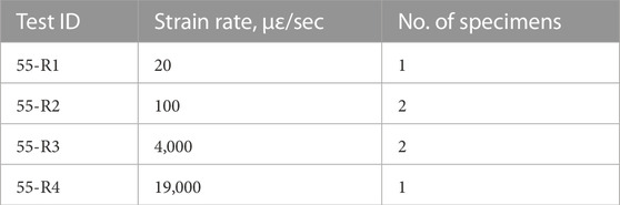
TABLE 1. Specimen description and test parameters.
2.2.1 Specimen preparation
The FRP pipes were manufactured in Little Rock, Arkansas by NOV Fiber Glass Systems, a producer of filament wound pipe for applications in the oil and gas, chemical, industrial, marine, and offshore industries (Fiber Glass Systems, 2018). The pipes were filament-wound with glass fibers oriented at ±55° with respect to the longitudinal axis of the tube. During the filament-winding process, the glass fibers were fed through an epoxy resin bath and deposited on a rotating steel mandrel. A CNC system controlled the movement to achieve the targeted fiber angle. Each layer consisted of fibers at both positive and negative orientations. The pipes were heat cured at 121°C for 75 min and then raised to 163°C for 45 min. The pipes were cooled to ambient temperature and cut to length prior to testing. Owens Corning Advantec® Type 30® rovings were used as the glass fiber reinforcement and an amine-cured epoxy resin was used as the polymer matrix. The FRP tubes had a tensile Modulus of Elasticity of 11.58 GPa, a hoop Modulus of Elasticity of 20.82 MPa, and a Poisson’s ratio of hoop strain to axial strain due to stress in the axial direction of 0.35, as specified by the manufacturer (Systems, 2012).
2.2.2 Test procedures and instrumentation
The experimental setup and instrumentation are shown in Figure 1A. The specimens were loaded with a spherical bearing to provide a moment-free end condition. The overall displacement of the loading platen was measured by two 50-mm stroke displacement transducers. The transducers were centered on opposite sides of the tubes. Local strains were measured by triaxial strain gauge rosettes on the side of the column at mid-height (Figure 1A). The gauges were 5 mm and at angles of 0°, 45°, and 90° as shown in Figure 1B. All specimens were tested in a Satec 1780 kN hydraulic testing machine.
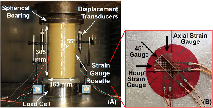
FIGURE 1. Representative view of (A) typical test setup and (B) rosette strain gauge.
A displacement-based loading protocol was defined by targeting axial strains given the average reading from the displacement transducers. Additional time was added between loading cycles so that the total loading time per cycle was equivalent for each loading rate. This also allowed the stress relaxation under constant axial strain to be measured. A representative loading protocol is shown in Figure 2, with compressive strains shown as positive. The first cycle targeted 0.5% strain and the subsequent cycles increased by 1.0% strain. The cyclic compression continued with increasing targets until the FRP tube ruptured or the resistance of the specimens dropped to 50% of the peak load.
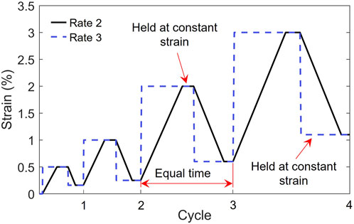
FIGURE 2. Representative loading protocol.
2.2.3 Stress-strain relationships and motivation for modeling approach
Sample stress-strain relationships for each rate are shown in Figure 3, according to the average axial strain gauge readings. Compression is shown as positive, and tension is shown as negative. The backbone curves are compared in Figure 4A. For presentation purposes, only one response is shown for each rate as the repeated tests (i.e., 55-R2 and 55-R3) resulted in comparable responses. The results demonstrate that as the loading rate increases, the stiffness and peak stresses increase. The failure strains were comparable for the different rates, with all specimens failing around 3.0% strain. Additionally, rates 3 and 4 are shown to have comparable stiffnesses, despite rate 4 being approximately five times larger than rate 3.
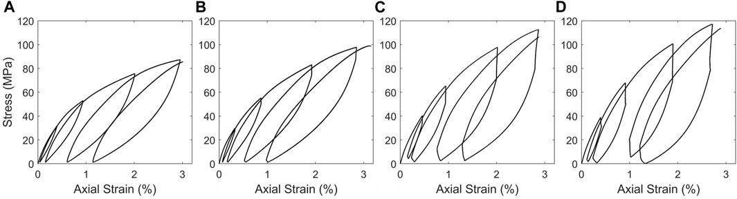
FIGURE 3. Experimental stress-strain response for specimens (A) 55-R1, (B) 55-R2, (C) 55-R3, and (D) 55-R4.
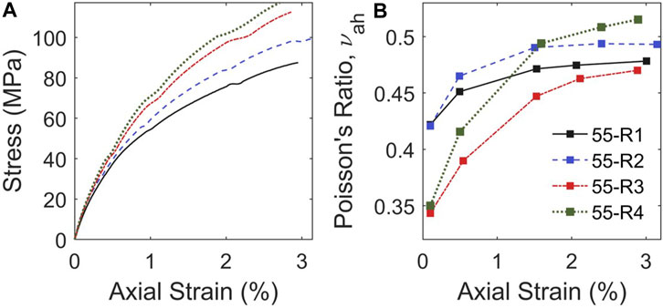
FIGURE 4. Experimental results including (A) stress-strain envelope curve and (B) Poisson’s ratio.
Figure 4B shows the Poisson’s ratio, νah, calculated as the ratio of hoop to axial strain and plotted against the axial strain. The first point was calculated in the elastic region and the succeeding points were taken as the average ratios while the pipes were being loaded. It is plotted against the average axial strain during corresponding times. Figure 4B demonstrates that Poisson’s ratio initially decreased as the loading rate increases. This is consistent with previous findings for filament-wound FRP tubes with fibers oriented at ±55°, which found Poisson’s ratio of 0.28 and 0.43 for loading rates of approximately 270 and 23 kPa/s, respectively (Carroll et al., 1995). While the laminate properties of the specimens differed, the trend for the elastic properties is consistent with the observations in Figure 4B. In the current study, the Poisson’s ratio increased as the axial strain increased in the subsequent loading cycles, with a more substantial increase for the high loading rates, rate 3 and rate 4. As such, the relationship between axial strain and hoop strain has rate-dependent behavior. These observations were used to develop a macro-scale modeling methodology that captured the nonlinear and rate-dependent behavior of the FRP tubes as well as the interaction of hoop and axial strains, which is detailed in the following sections.
2.3 Analytical modeling
An analytical model was developed to capture the nonlinearity and rate-dependent behavior of the FRP tube as well as the interaction of axial and hoop strains. To accomplish this, an element configuration was defined with horizontal and vertical elements that represented the epoxy matrix and diagonal elements that represented the glass fibers. This approach allowed the nonlinearity and rate-dependent behavior observed experimentally to be represented by the matrix elements, distinct from the glass fibers, which remain largely elastic. Additionally, the interaction of axial-hoop deformations is inherently captured and the strain gauge measurements from the experimental investigation can be used for model verification. Figure 5 outlines the modeling approach. Figure 5A includes a view of the test setup and the relationship to the element configuration, which is detailed in Figure 5B. This configuration enables the nonlinear and viscoelastic behavior to be assigned to the elements representing the epoxy matrix and the diagonal elements to remain elastic (Figure 5B). Additionally, this configuration enables the relationship between axial and horizontal strain to be captured. As shown in Figure 5A, under axial compressive loads, the length, L, decreases and the diameter, D, increases. This deformation is shown in Figure 5C for the element configuration. The proposed modeling methodology can be easily updated for FRPs with different fiber or matrix properties as well as different fiber orientations.
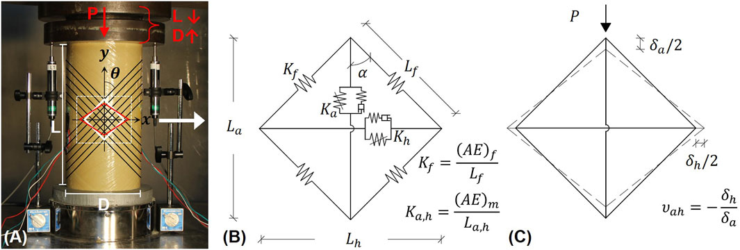
FIGURE 5. Overview of analytical modeling methodology including (A) motivation for element configuration due to deformation of length and diameter under axial loads, (B) schematic view of configuration including property definitions, and (C) deformation of elements under axial load and relationship to Poisson’s ratio.
The element properties and nonlinear behavior were determined in four parts. First, the in-plane material constants were calculated using the classical laminate for a given fiber angle. Next, the element properties for the proposed model were calculated given the elastic material properties. After verification of the elastic element model, a preliminary relationship capturing the nonlinear and rate-dependent behavior was defined and assigned to the elements representing the epoxy matrix (horizontal and vertical). Finally, the nonlinear and rate-dependent properties were calibrated using a previously proposed ML framework (Lanning et al., 2022). The simulated responses due to the CNN-predicted parameters were then verified using the experimental results. The following sections outline the procedure for obtaining the elastic properties as well as the details of the analytical model. After which, the ML-based calibration process is introduced and used to obtain the nonlinear properties for the analytical model.
2.3.1 Calculation of in-plane elastic properties for the FRP tube
The in-plane elastic properties of a FRP tube can be calculated for a given fiber winding angle, θ, with respect to the longitudinal axis, using the classical laminate theory. The approach previously suggested in (Hamed et al., 2008; Hain et al., 2019) for filament wound pipes was used to calculate the axial stiffness, Ea, hoop stiffness, Eh, Poisson’s ratio when loaded in the axial direction, νah, and Poisson’s ratio when loaded in the hoop direction, νha, using the unidirectional material properties. The general approach is detailed below with the results provided for the ±55° FRP tubes used in the current study.
The classical laminate theory can be used given the following assumptions: 1) the layers have the same materials, angles, and thicknesses, 2) the layup is balanced and symmetric, 3) the laminate of the cylindrical shell is constrained so that curvature and twist cannot change under uniform axis-symmetric loading, 4) the unidirectional layer is transversely isotropic in the 2–3 plane, 5) the shell acts as a thin-walled cylinder with negligible through-thickness effects, resulting in a plane stress condition. Given these assumptions, the FRP tube can be characterized with a 3 × 3 stiffness matrix using only four unidirectional material properties, E1, E2, v12, and G12, where direction 1 is parallel to the fibers and direction 2 is perpendicular to the fibers. The stiffness matrix is shown in Eq. 1 relating the stress and strain in the principal material directions using Hook’s law for a single unidirectional lamina of an orthotropic material.
where:
The four unidirectional properties were calculated using the fiber and matrix properties. The longitudinal fiber and matrix moduli were 81 GPa and 3.2 GPa, respectively, and the fiber volume faction was 0.6, obtained from the manufacturer. The fiber and matrix Poisson’s ratios were assumed to be 0.23 and 0.35, respectively, based on suggested typical values (Daniel et al., 1994). The rule of mixtures was used to calculate the longitudinal modulus and Poisson’s ratio, E1 and v12, using Eqs 2, 3, respectively. The rule of mixtures typically underestimates the transverse modulus, E2, and in-plane shear modulus, G12, which are matrix-dominated properties. To combat this, Halpin-Tsai’s relationships were used, shown in Eqs 4, 5, for ξ = 1, as suggested by (Daniel et al., 1994) based on experimental testing. As glass fibers are isotropic, the longitudinal fiber modulus was replaced with the transverse fiber modulus, E2f. The unidirectional properties, E1, E2, v12, and G12, were calculated to be 49.9 GPa, 11.16 GPa, 0.278, and 4.18 GPa, respectively.
Next, the classical laminate theory was applied to calculate the in-plane elastic properties given the previously reported unidirectional properties and a fiber angle of 55°, following the approach detailed in (Hamed et al., 2008; Hain et al., 2019). This is accomplished by transforming the stress-strain relationships from the material to the loading directions to obtain the hoop and axial properties given the specified fiber angle. These relationships are shown in Eq. 6. The in-plane elastic constants are solved for using Eqs 7–10 with the results provided in Table 2. The calculated properties have close agreement to the manufacturer’s reported properties (Systems, 2012), which are included in Table 2 for comparison. The calculated in-plane properties were used in the subsequent calculations for the proposed element configuration.
where:

TABLE 2. Calculated versus specified in-plane properties.
2.3.2 Calculation of properties for proposed element configuration
The in-plane elastic properties of the FRP tube (Ea, Eh, νah, νha) were used to calculate the elastic properties for the proposed element configuration. These include the element stiffnesses, K, and angle, α, defined in Figure 5B. The subscript f is used to indicate the section properties for the diagonal elements, which represent the glass fibers. The subscripts a and h indicate the axial and hoop elements, respectively. As the horizontal and vertical elements both represent the epoxy matrix, the section properties, Aa,h and Ea,h, are replaced by (AE)m. The resulting fiber and matrix element stiffnesses are defined in Eqs 11, 12, respectively.
The values for AEf, AEm, and α, were solved for by applying a unit load, assuming length of 1 for Lf, and enforcing equilibrium in the x-direction, equilibrium in the y-direction, and displacement compatibility. This was repeated for a vertical unit load and horizontal unit load given the known in-plane elastic constants. The deformed shape under a vertical unit load is shown in Figure 5C. The value for α was calculated separately from the given fiber angle of ±55° to ensure the relationship between horizontal and vertical deformations could be enforced. The calculated values for AEf, AEm, and α were 37.1 GPa, 8.6 GPa, and 56.4°, respectively, given the calculated in-plane properties previously reported in Table 2.
2.3.3 Analytical model setup
The analytical modeling was performed in OpenSees, which is an open-source, object-oriented structural analysis framework (Mazzoni et al., 2006). The element configuration defined in Figure 5B was modeled in OpenSees using a truss element object to define the vertical, horizontal, and diagonal elements. The schematic view of the nonlinear analytical model is shown in Figure 6 along with the element types, material commands, and constitutive material models. The model parameters to be calibrated with the ML framework are shown in boldface in Figure 6 and summarized in Table 3. The measured axial strain was used as the input displacement in the analytical model and the resulting axial stress and hoop strain were recorded. The general analytical model details are discussed below, with a focus on the parameters requiring calibration.
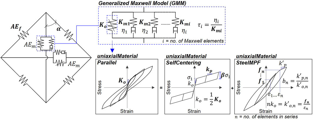
FIGURE 6. Schematic view of the nonlinear analytical model of a FRP composite tube. The mechanistic rheological model for the GMM is shown consisting of a nonlinear spring element and i Maxwell elements. The OpenSees material commands are identified along with the general shape of the hysteresis curves. The parameters to be calibrated are shown in boldface.
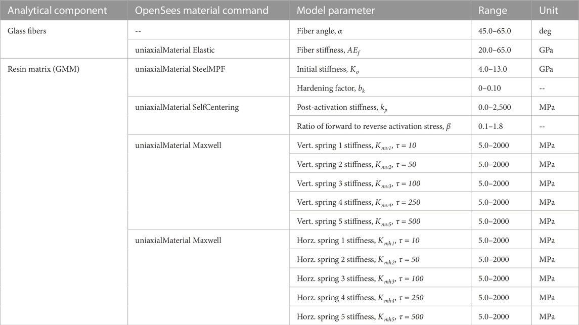
TABLE 3. Details of model parameters to be calibrated by the CNN, including the modeling component, interval of input values, and OpenSees commands.
Prior to defining the nonlinear relationships, the elastic response was verified for the model configuration under a unit axial load for the calculated properties, AEf, AEm, and α. The section properties, AEf and AEm, were assigned to the uniaxial material “Elastic”, and used to define the fiber and epoxy matrix properties. The angle, α, was used to define the length of the elements, consistent with the calculations discussed previously. After verification of the elastic properties, the nonlinear and viscoelastic behavior were defined for the epoxy matrix using the generalized Maxwell model (GMM), which is commonly used to represent viscoelastic materials (Christensen, 2012; Findley and Davis, 2013). The GMM consists of multiple Maxwell models assembled in parallel with a single spring element, as shown in Figure 6. A single Maxwell model is composed of an elastic spring and a viscous dashpot connected in series. The GMM combines multiple Maxwell models, permitting the stress relaxation to occur in a set of times, not only at a single time. Five Maxwell elements were initially defined in the GMM, and the ML framework was used to determine the spring stiffness, Km, of each Maxwell element. The relaxation time, τ, was fixed and differed for each Maxwell element. As such, the Km could be decreased by the ML framework if an irrelevant relaxation time was selected, simplifying the number of parameters predicted by the framework. The Km values were separate for the horizontal and vertical elements, resulting in a total of 10 Mx models initially defined. The viscoelastic parameters for the horizontal and vertical components were left independent to enable capturing the rate-dependent behavior of the Poisson’s ratio observed in the experimental results as well as in previous studies (Suchocki and Molak, 2019). After calibration, the inconsequential Maxwell elements in the GMM were removed (i.e., elements with Km values <100 MPa) to simplify the model. This process is discussed further in the results and discussion section.
The nonlinear spring element in the GMM was defined with a uniaxial material to represent the nonlinear behavior of the matrix (Figure 6). Due to the limitations of the available uniaxial material models within OpenSees, multiple material models were used to capture the nonlinear hysteresis response. The configuration of the uniaxial materials representing the nonlinear spring in the GMM is shown in Figure 6. This setup included a combination of the uniaxial materials “SteelMPF” and “SelfCentering” to capture the hysteresis shape while enforcing the recentering behavior of the FRP tube. The response of specimen 55-R1 was used to define the preliminary envelope curve for the uniaxial materials. This ensured the general shape was captured prior to adding the viscoelastic components and generating the analytical training dataset. The hysteresis response for “SteelMPF”, “SelfCentering”, and the combined response when in parallel is shown in Figure 6 along with the constitutive relationships. To capture the gradual yielding, four “SteelMPF” materials were defined in series with progressive yielding points. The parameters to be calibrated for each uniaxial material are in Table 3. To simplify the number of parameters requiring calibration, the hardening ratios, b, for the four “SteelMPF” materials were defined to approximate the envelope curve for specimen 55-R1. The hardening ratios were then shifted uniformly by a single constant, bk, which was included as a calibration parameter in the framework. A total of 16 analytical model parameters requiring calibration were included and defined as target variables when training a CNN. The ranges of the parameters, as shown in Table 3, were selected to encompass the expected values estimated through specified or calculated material properties, material testing, and engineering judgment (Wilson, 2004; Shao et al., 2005; Systems, 2012; Zaghi et al., 2012).
2.4 Parameter calibration using convolutional neural networks
The ML framework proposed by Lanning et al. (Lanning et al., 2022) was adapted and used in this study to obtain the model parameters for the FRP tubes tested under variable loading rates. In the framework, the analytical model that was previously calibrated given the elastic properties of the model through unit axial loads was subsequently used to generate a dataset of simulations given different permutations of the nonlinear or rate-dependent parameters that require calibration. The synthetic dataset was then used to train a CNN to predict the model parameters. Next, the trained CNN was prompted with the experimental data to obtain the calibrated parameters. The experimental data is effectively used as a new task for the network, with the advantage that it shares underlying principles and structures with the synthetic data. This method exploits the network’s ability to learn from a large amount of synthetic data and apply that knowledge to understand and predict from a small amount of experimental data. To accomplish this, the experimental responses of specimens tested under rates 2 and 3 were used for prompting. The average predicted parameters were used to generate the analytical response for the four loading rates. The following sections discuss details of the ML framework, including generation of the synthetic dataset, network architecture, and network validation.
2.4.1 Generation of the synthetic dataset
The analytical model previously introduced was used to generate a dataset of 30,000 analytical simulations for training the CNN given different permutations of the parameters requiring calibration. A quasi-random number generator was used to define these parameters within the bounds shown in Table 3. A quasi-random number generator was implemented as it minimizes discrepancy between generated points to fill the multi-dimensional space in a uniform manner (Skublska-Rafajłowicz and Rafajłowicz, 2012; Sobol', 1967; Matoušek, 1998). This results in the synthetic dataset containing a comprehensive representation of the 16 parameters and their effect on the predicted response. The quasi-random number dataset was generated using the Sobol sequence (Sobol', 1967). The first 1,000 points were omitted, and the sequence was scrambled using Owen’s scrambling algorithm to reduce correlations and improve uniformity (Matoušek, 1998).
In addition to the model parameters, the input axial strain was varied within the synthetic dataset. This was done to incorporate the variations in the loading protocols, such as the loading rate and differences in achieved displacements during the loading and unloading cycles. A representative sample set of the loading protocols are shown in Figure 7 in addition to the idealized loading protocols for specimens 55-R2 and 55-R3 for reference. The relationship between the axial and hoop strains was varied by randomly adjusting the recorded hoop strain amplitude by ±5%. This introduced additional noise to the training data to mitigate overfitting and improve performance for the experimental data.
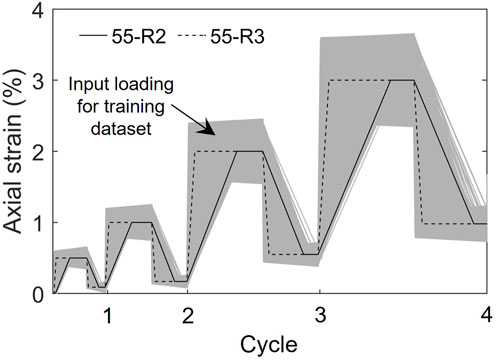
FIGURE 7. Sample set of loading protocols used to generate synthetic dataset for training the CNN.
The input axial strain and resulting stress and hoop strain from the analytical model were used to train the CNN. The input data was reshaped into a 2D array following the data preparation approach suggested in (Lanning et al., 2022). In this approach, the cell data representing the amplitude is used to define pixel intensity for an image when processed by a CNN. The signal amplitudes were rescaled to an integer from 0 to 255, representing pixel intensity. The 2D arrays for the axial strain, hoop strain, and axial stress time histories were concatenated into the red, green, and blue color channels to create a single RGB image for a given analytical simulation. This resulted in a single input image corresponding to the model parameters for training a CNN.
2.4.2 Network architecture
CNN architectures typically contain an image input layer, convolutional layers, and an output layer. Each convolution layer uses a kernel to extract features from local regions of the input. The kernel is a matrix of weights that slides across the input and is convolved with the pixels from a small area of the input to form the output feature maps. The CNN architecture for the current study is depicted in Figure 8, as well as a representative input image, which included the axial strain, hoop strain, and axial stress arrays. The CNN architecture in this work included three convolution layers with kernel sizes of 3 × 3. Zero-padding was used so that the convolution layers did not alter the spatial dimensions of the input. Each convolution layer included rectified linear unit (ReLU) as the activation function, which introduced nonlinearity to the system. Each convolution layer was succeeded by a pooling layer, which down-sampled values in the feature maps to reduce the number of parameters and dimensionality of the feature maps. A pooling size and stride of 1 × 2 was used, which down-sampled the adjacent points in the time-history without distorting the order. A dropout rate of 20% was introduced prior to the fully connected layer as a regularization method to prevent overfitting (Srivastava et al., 2014). Finally, a fully connected layer was used to convert the feature map into a feature vector the size of the number of output variables. As the data was synthetically generated, a large dataset with 30,000 samples was used in this study.
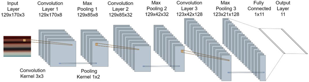
FIGURE 8. CNN architecture.
The synthetic dataset was divided into training, validation, and testing subsets using an 80/15/5 split. The Adam optimization algorithm (Kingma and Ba, 2014) was used with an initial learning rate of 0.001, which decreased by a factor of 0.1 every 10 epochs. The validation dataset was used to calculate accuracy and loss during training to monitor the progress. Root mean-squared-error (RMSE) was defined as the loss function. Early stopping was used to automatically terminate training when the current validation loss had exceeded the lowest validation loss 10 times.
2.4.3 Validation of the trained CNN
The performance of the CNN was assessed using the accuracy capturing the model parameters for the testing dataset as well as the validation RMSE and loss, which were measured during training. The testing dataset included 5% of the synthetic dataset and was unseen during training to prevent overfitting. The trained network had a validation RMSE and loss of 0.43 and 0.11, respectively. The predicted model parameters had an average R2 value of 0.93 for the training set, 0.92 for the testing set, and 0.89 for the validation set. The accuracy of the network during training lowered when random noise was added to the synthetic dataset. However, the performance decrease was insignificant for the testing dataset and the accuracy difference between the data subsets was lessened, indicating the addition of noise decreased overfitting and improved the capability to generalize. As a result, the accuracy capturing the experimental responses also improved.
The model parameters for the FRP pipes were obtained by prompting the trained network with the experimentally measured axial strain, hoop strain, and axial stress. The experimental responses for the specimens loaded under rates 2 and 3 (55-R2 and 55-R3) were used to obtain the calibrated parameters. This included two specimens tested under each rate, resulting in four sets of predicted parameters. The values were averaged and used to generate the analytical responses for the specimens tested under all four rates (i.e., 55-R1, 55-R2, 55-R3 and 55-R4.) This was done to evaluate the accuracy capturing the response of specimens tested with rates outside of the range used for prompting.
3 Results and discussion
3.1 Predicted response of FRP tubes
The experimental responses for the specimens loaded under the rates 2 and 3 were fed to the trained network to obtain the calibrated parameters. The predicted parameters were all within the range of estimated values from material testing, constitutive equations, or manufacturer specifications. This indicates that the network did not compensate with unrealistically large or small values when prompted with experimental data. Table 4 includes the average model parameters as well as the average values for the four specimens tested under rates 2 and 3, for comparison. The standard deviation and coefficient of variance (COV) are also reported in Table 4, as the COV permits comparison of the variance between parameters with different units. Within the GMM, the Maxwell elements with Km values less than 100 MPa were removed as they had a negligible effect on the response. As previously discussed, these elements were initially included to allow the relaxation time, τ, to be calibrated without including it as a direct training parameter. As removing these parameters had a negligible effect on the predicted response, a new network was not trained. The parameters for the remaining Maxwell elements are reported included in Table 4 for simplicity. The predicted values for the nonlinear parameters were comparable between the two rates, i. e., the parameters defined uniaxial materials “SteelMPF” and “SelfCentering”. In contrast, the viscoelastic parameters assigned to the Maxwell elements had the largest COV of the calibrated parameters. This was anticipated as the Maxwell elements with lower relaxation times (τ < 50 s) have a less substantial effect on the response under the slower loading rates. Despite the limited effect, the trained network predicted reasonable values without greatly over-predicting or underpredicting. This suggests some information was encoded into the time history, despite the limited effect on the global response. However, if the model is anticipated to be used for various loading rates, it is suggested that a range of loading rates be obtained experimentally and used for model validation.
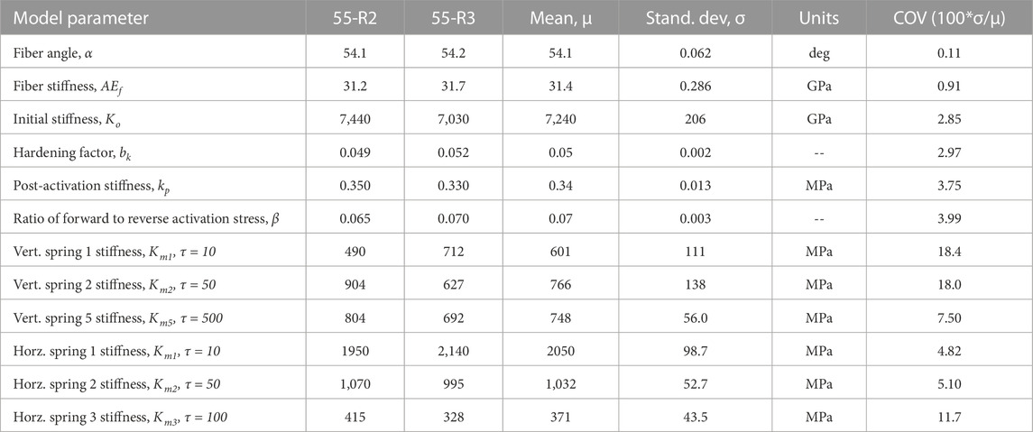
TABLE 4. Predicted model parameters given the experimentally measured responses.
The predicted parameters for specimens 55-R2 and 55-R3 were averaged and used in the OpenSees analytical model to simulate the response of the FRP tube under the four loading rates, as previously discussed. The resulting responses are shown in Figure 9, including the axial stress-axial strain hysteresis, axial stress-hoop strain hysteresis, and the stress time history. The predicted Poisson’s ratios are compared to the measured values in Figure 10. The global axial stress-strain responses were successfully captured for the two loading rates used for calibration as well as under rates 1 and 4. The R2 values were calculated for the axial stress and hoop strain time histories given the measured and predicted responses to quantify the accuracy across the time history. The R2 values for the axial stress time histories were 0.982, 0.995, 0.994, and 0.992 for specimens 55-R1, 55-R2, 55-R3, and 55-R4, respectively. The R2 values for the hoop strain time histories were 0.987, 0.997, 0.997, and 0.984 for specimens 55-R1, 55-R2, 55-R3, and 55-R4, respectively. Overall, the accuracy was higher for the specimens used to calibrate the model parameters (55-R2 and 55-R3). The high accuracy simulating the response of specimens 55-R1 and 55-R4 demonstrated the calibrated parameters are applicable outside of the rates used for prompting. This accuracy is attributed to adequate information on the full range of loading rates being included in the large synthetic training dataset.
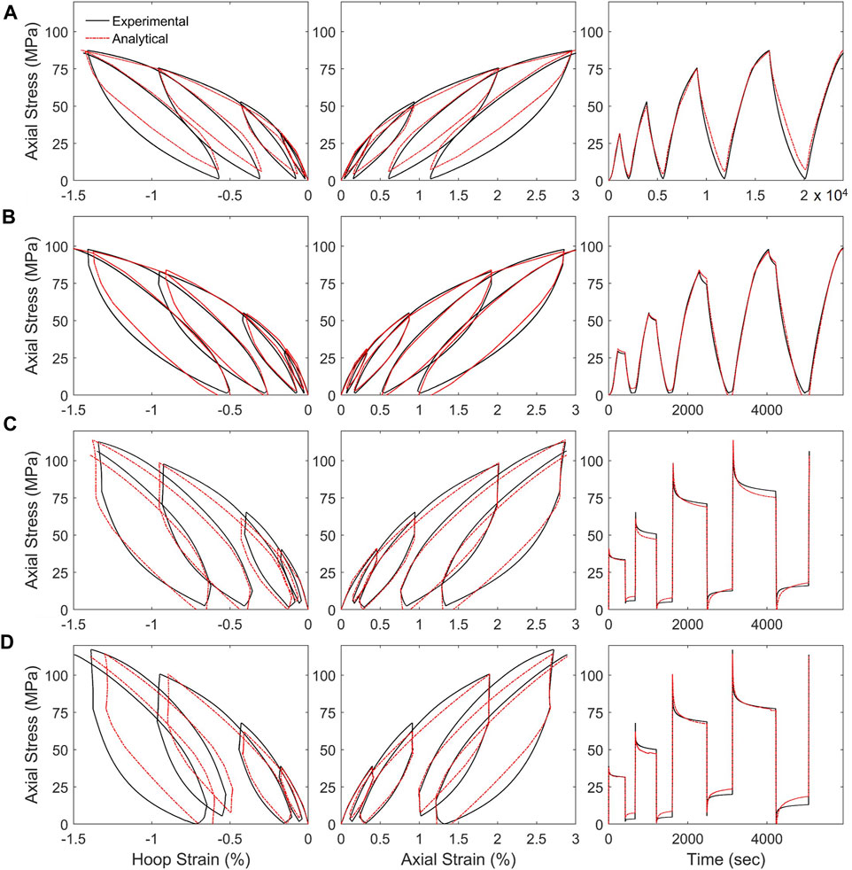
FIGURE 9. Experimental responses versus modeled responses including axial stress-hoop strain, axial stress-strain, and stress time history for specimens (A) 55-R1, (B) 55-R2, (C) 55-R3, and (D) 55-R4.
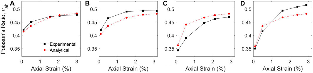
FIGURE 10. Poisson’s ratio of experimental and modeled responses for specimens (A) 55-R1, (B) 55-R2, (C) 55-R3, and (D) 55-R4.
3.2 Response under biaxial loading conditions
The analytical model was used to investigate the effects of biaxial loading and variations in the fiber orientation for angles between ±45° and ±70°. Biaxial loading was simulated by applying simultaneous strain time histories in both the axial and hoop directions. The hoop strain was applied proportionally to the axial strain for strain ratios (εh/εa) between 0.4 and 0.55. This is relevant for applications such as in CFFT columns, where the FRP tube provides confinement to the concrete core. After unconfined concrete reaches stresses of approximate 0.7f′c, the apparent Poisson’s ratio (or strain ratio εh/εa) of concrete increases from approximately 0.2–0.5 (Elwi and Murray, 1979; Mirmiran and Shahawy, 1997). The compressive strength, f’c, of concrete typically varies between 17 MPa and 35 MPa, which corresponds to 0.7f′c of 8.5 MPa and 17.5 MPa, respectively. At this point, the concrete core will impose a hoop strain, εh, onto the FRP tube. For this study, the strain ratio was assumed to be constant, and the response of an FRP tube was simulated for four ratios, as shown in Figure 11A. These results are compared to the unconstrained case, i.e., where εh is free to displacement based on the FRP properties. The strain rate was approximately 100 µε/sec, comparable to strain rate 2 from the experimental program. For the unconstrained case (εh = free), the initial stiffness and early cycles are comparable to the response under εh= 0.4εa, as shown in Figure 11B. After achieving axial strains of approximately 0.3%, the unconstrained response is comparable to the response for εh= 0.45εa and subsequently εh= 0.5εa, as indicated in Figure 11B. This reflects the variation in the measured Poisson’s ratio from 0.4 to 0.5 for specimen 55-R2, as shown in Figure 4B. If the applied strain ratio was less than the measured Poisson’s ratio, the strain in the hoop direction was partially constrained, resulting in a larger stiffness. Strain ratios above the measured Poisson’s ratio resulted in biaxial loading conditions where, for the example of a CFFT column, additional hoop displacement occurs due to crushing of the concrete core. These cases resulted in a lower axial stiffness as the hoop direction was displacing faster than in the unconstrained case.
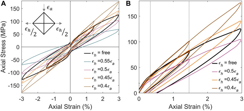
FIGURE 11. Effect of biaxial loading due to proportionally applied hoop strain showing the (A) full hysteresis response (B) zoomed view of the early cycles.
The response when strain in the hoop direction is fully constrained, i.e., εh = 0, is shown in Figure 12. This response is compared to the calculated elastic stiffness according to the schematic setup in Figure 5B. As shown in Figure 12, the response is fiber-dominant, with slight nonlinear behavior due to the epoxy matrix.
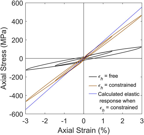
FIGURE 12. Response when strain in hoop direction is constrained compared to then response when strain in hoop direction is free and the calculated response assuming elastic behavior.
3.3 Future applications
The developed modeling methodology and the ML-based approach in this study have broad applications for analyzing structures made of filament-wound FRP tubes, such as piping systems and CFFT elements. The advanced and intricate behavior of FRP materials under variable rates of loading, including their rate-dependent, viscoelastic and nonlinear behavior, are captured accurately by the proposed model, which provides a solid foundation for their structural analysis and design. The proposed FRP model uses classical laminate theory to calculate the elastic properties based on the specified fiber orientation. It can thus be used to evaluate the performance of FRP pipes with different fiber winding angles under the same loading conditions. By running simulations for various fiber orientations and laminate thicknesses, the model can help identify configurations that maximize the load-carrying capacity and durability of the FRP tube for a given application. This could be used as an optimization tool during the design phase.
For FRP piping systems commonly used in civil, chemical, and petroleum industries, the analytical model could offer insightful understanding of the response of the piping system under various loading rates, such as wind pressure, water, and other in-service loads. The rate-dependent viscoelastic behavior can be significant for FRP piping systems, especially when they are exposed to high velocity dynamic loadings, cyclic loadings, or long-term loads. Therefore, the considered ML-calibrated model can provide better predictions of the safety and long-term performance of FRP pipes. The most common loading on FRP piping systems is internal pressure due to the fluid flowing through the pipe. The model considers the element configuration that represents the matrix and fiber elements. The biaxial loading on the piping system can be modeled directly and can simulate the response of the FRP tube under uniform internal pressure, which results in biaxial stresses in the tube wall. The model can also be extended to consider additional loads that may act on FRP piping systems, such as external pressure, bending and axial loads, allowing the interaction between the various loading effects on the strains and stresses in the FRP tube wall to be captured.
For CFFT elements, this modeling methodology allows a more accurate representation of their structural behavior under static and dynamic loads. These elements are frequently used in civil engineering applications due to their high strength-to-weight ratios and superior corrosion resistance. However, the simulation of these structures is complex due to the viscoelastic behavior of the composite materials and the interaction between concrete and FRP tubes. For modeling CFFTs, a similar approach as the FRP model can be followed to define the concrete core. A variation of the element configuration as shown in Figure 5B can be used with parameters calibrated to capture the rate-dependent behavior of the concrete material. The two models can be integrated so that the top and bottom nodes are connected with rigid elements and the horizontal movement or hoop strain are tied so that the FRP tube and concrete experience the same hoop strain. While the calibration of the concrete core requires extensive simulations and is outside the scope of the current work, the same framework may be used.
4 Conclusion
This work proposed a novel modeling methodology to represent the short-term viscoelastic properties of FRP tubes as well as the nonlinear cyclic response and interaction of axial and hoop strains. Experimental testing of filament-wound FRP tubes with winding angle of ±55° under cyclic axial compression was used for model validation. The FRP tubes exhibited viscoelastic behavior, including stress relaxation under constant strain and a dependence of stress on the strain rate. A previously proposed supervised ML framework was modified to calibrate the model parameters with limited experimental data. The framework consisted of training a CNN using a synthetic dataset to learn the relationships between the analytical model parameters and the axial stress, axial strain, and hoop strain time histories. The trained CNN had a validation RMSE and loss of 0.43 and 0.11, respectively. The predicted model parameters had an average R2 value of 0.93 for the training set, 0.92 for the testing set, and 0.89 for the validation set. The trained network was prompted with the experimental data to obtain analytical model parameters for the FRP tubes that are applicable to a range of loading rates. The results of the study demonstrated a CNN can perform parameter calibration for nonlinear models of composites and calibrate rate-dependent properties.
When prompted with the experimental data, the trained CNN predicted reasonable model parameters and captured the measured response of the FRPs over the range of loading rates. The modeling methodology successfully simulated the nonlinear cyclic response of the FRP tubes, including the viscoelastic behavior due the epoxy matrix and the relationship of axial and hoop strains. The accuracy capturing the measured stress-strain responses demonstrated the synthetic dataset was adequate for training the CNN without requiring additional experimental data. The proposed FRP modeling methodology was used to investigate the response under biaxial loading. Additional research is needed to evaluate the applicability of the model to various fiber orientations and architectures.
Data availability statement
The raw data supporting the conclusion of this article will be made available by the authors, without undue reservation.
Author contributions
AL and AZ conceptualized the work. AL implemented the program and wrote the manuscript with input from AZ. All authors contributed to the article and approved the submitted version.
Funding
This project was supported by the National Science Foundation Partnership for Innovation Award #1500293. The student support for this project was funded by the National Science Foundation Graduate Research Fellowship under Grant No. 1747453.
Acknowledgments
The authors acknowledged the guidance of Dr. Hadi Meidani of the University of Illinois at Urbana-Champaign. The support of Dr. Alexandra Hain of the University of Connecticut, Tao Zhang, and Michael Vaccaro Jr is also appreciated.
Conflict of interest
The authors declare that the research was conducted in the absence of any commercial or financial relationships that could be construed as a potential conflict of interest.
Publisher’s note
All claims expressed in this article are solely those of the authors and do not necessarily represent those of their affiliated organizations, or those of the publisher, the editors and the reviewers. Any product that may be evaluated in this article, or claim that may be made by its manufacturer, is not guaranteed or endorsed by the publisher.
References
Carroll, M., Ellyin, F., Kujawski, D., and Chiu, A. (1995). The rate-dependent behaviour of±55 filament-wound glass-fibre/epoxy tubes under biaxial loading. Compos. Sci. Technol.55, 391–403. doi:10.1016/0266-3538(95)00119-0
Chandra Ray, B., and Rathore, D. (2015). A review on mechanical behavior of FRP composites at different loading speeds. Crit. Rev. solid state Mater. Sci.40, 119–135. doi:10.1080/10408436.2014.940443
Chen, C.-T., and Gu, G. X. (2019). Machine learning for composite materials. MRS Commun.9, 556–566. doi:10.1557/mrc.2019.32
Chen, J., Wan, L., Ismail, Y., Ye, J., and Yang, D. (2021). A micromechanics and machine learning coupled approach for failure prediction of unidirectional cfrp composites under triaxial loading: A preliminary study. Compos. Struct.267, 113876. doi:10.1016/j.compstruct.2021.113876
Daniel, I. M., Ishai, O., Daniel, I. M., and Daniel, I. (1994). Engineering mechanics of composite materials. New York: Oxford University Press.
Daniel, I., Werner, B., and Fenner, J. (2011). Strain-rate-dependent failure criteria for composites. Compos. Sci. Technol.71, 357–364. doi:10.1016/j.compscitech.2010.11.028
Elwi, A. A., and Murray, D. W. (1979). A 3D hypoelastic concrete constitutive relationship. J. Eng. Mech. Div.105, 623–641. doi:10.1061/jmcea3.0002510
Fallahi, H., Taheri-Behrooz, F., and Asadi, A. (2020). Nonlinear mechanical response of polymer matrix composites: A review. Polym. Rev.60, 42–85. doi:10.1080/15583724.2019.1656236
Fiber Glass Systems (2018). National oilwell varco. [Online]. Available at: https://www.nov.com/Segments/Completion_and_Production_Solutions/Fiber_Glass_Systems.aspx (Accessed, 2018).
Findley, W. N., and Davis, F. A. (2013). Creep and relaxation of nonlinear viscoelastic materials. Chelmsford: Courier Corporation.
Gandomi, A. H., Babanajad, S. K., Alavi, A. H., and Farnam, Y. (2012). Novel approach to strength modeling of concrete under triaxial compression. J. Mater. Civ. Eng.24, 1132–1143. doi:10.1061/(asce)mt.1943-5533.0000494
Gates, T. S. (1992). Experimental characterization of nonlinear, rate-dependent behavior in advanced polymer matrix composites. Exp. Mech.32, 68–73. doi:10.1007/bf02317988
Goh, S., Charalambides, M., and Williams, J. (2004). Determination of the constitutive constants of non-linear viscoelastic materials. Mech. Time-Dependent Mater.8, 255–268. doi:10.1023/b:mtdm.0000046750.65395.fe
Gu, G. X., Chen, C.-T., Richmond, D. J., and Buehler, M. J. (2018). Bioinspired hierarchical composite design using machine learning: Simulation, additive manufacturing, and experiment. Mater. Horizons5, 939–945. doi:10.1039/c8mh00653a
Hain, A., Motaref, S., and Zaghi, A. E. (2019). Influence of fiber orientation and shell thickness on the axial compressive behavior of concrete-filled fiber-reinforced polymer tubes. Constr. Build. Mater.220, 353–363. doi:10.1016/j.conbuildmat.2019.05.194
Hamed, A. F., Megat, M., Sapuan, S., and Sahari, B. (2008). Theoretical analysis for calculation of the through thickness effective constants for orthotropic thick filament wound tubes. Polymer-Plastics Technol. Eng.47, 1008–1015. doi:10.1080/03602550802353144
Kingma, D. P., and Ba, J. (2014). Adam: A method for stochastic optimization. arXiv preprint arXiv:1412.6980.
Kiranyaz, S., Avci, O., Abdeljaber, O., Ince, T., Gabbouj, M., and Inman, D. J. (2021). 1D convolutional neural networks and applications: A survey. Mech. Syst. Signal Process.151, 107398. doi:10.1016/j.ymssp.2020.107398
Kujawski, D., and Ellyin, F. (1995). Rate/frequency-dependent behaviour of fibreglass/epoxy laminates in tensile and cyclic loading. Composites26, 719–723. doi:10.1016/0010-4361(95)91139-v
Lanning, A., Zaghi, E. A., and Zhang, T. (2022). Applicability of convolutional neural networks for calibration of nonlinear dynamic models of structures. Front. Built Environ.8. doi:10.3389/fbuil.2022.873546
Liu, X., Gasco, F., Goodsell, J., and Yu, W. (2019). Initial failure strength prediction of woven composites using a new yarn failure criterion constructed by deep learning. Compos. Struct.230, 111505. doi:10.1016/j.compstruct.2019.111505
Matoušek, J. (1998). On thel2-discrepancy for anchored boxes. J. Complex.14, 527–556. doi:10.1006/jcom.1998.0489
Mazzoni, S., Mckenna, F., Scott, M. H., and Fenves, G. L. (2006). OpenSees command language manual. Berkeley: University of California, Berkeley.
Mirmiran, A., and Shahawy, M. (1996). A new concrete-filled hollow FRP composite column. Compos. Part B Eng.27, 263–268. doi:10.1016/1359-8368(95)00019-4
Mirmiran, A., and Shahawy, M. (1997). Dilation characteristics of confined concrete. Mech. Cohesive-frictional Mater.2, 237–249. doi:10.1002/(sici)1099-1484(199707)2:3<237::aid-cfm32>3.0.co;2-2
Nguyen, S.-N., Truong-Quoc, C., Han, J.-W., Im, S., and Cho, M. (2021). Neural network-based prediction of the long-term time-dependent mechanical behavior of laminated composite plates with arbitrary hygrothermal effects. J. Mech. Sci. Technol.35, 4643–4654. doi:10.1007/s12206-021-0932-2
Paul, A., Acar, P., Liao, W.-K., Choudhary, A., Sundararaghavan, V., and Agrawal, A. (2019). Microstructure optimization with constrained design objectives using machine learning-based feedback-aware data-generation. Comput. Mater. Sci.160, 334–351. doi:10.1016/j.commatsci.2019.01.015
Qiu, C., Han, Y., Shanmugam, L., Zhao, Y., Dong, S., Du, S., et al. (2021). A deep learning-based composite design strategy for efficient selection of material and layup sequences from a given database. Compos. Sci. Technol.230, 109154. doi:10.1016/j.compscitech.2021.109154
Qvale, D., and Ravi-Chandar, K. (2004). Viscoelastic characterization of polymers under multiaxial compression. Mech. time-dependent Mater.8, 193–214. doi:10.1023/b:mtdm.0000046749.79406.f5
Sadoughi, M., and Hu, C. (2019). Physics-based convolutional neural network for fault diagnosis of rolling element bearings. IEEE Sensors J.19, 4181–4192. doi:10.1109/jsen.2019.2898634
Shao, Y., Aval, S., and Mirmiran, A. (2005). Fiber-element model for cyclic analysis of concrete-filled fiber reinforced polymer tubes. J. Struct. Eng.131, 292–303. doi:10.1061/(asce)0733-9445(2005)131:2(292)
Shao, Y., and Mirmiran, A. (2004). Nonlinear cyclic response of laminated glass FRP tubes filled with concrete. Compos. Struct.65, 91–101. doi:10.1016/j.compstruct.2003.10.009
Skublska-Rafajłowicz, E., and Rafajłowicz, E. (2012). Sampling multidimensional signals by a new class of quasi-random sequences. Multidimensional Syst. Signal Process.23, 237–253. doi:10.1007/s11045-010-0120-5
Sobol', I. Y. M. (1967). On the distribution of points in a cube and the approximate evaluation of integrals. Zhurnal Vychislitel'noi Mat. i Mat. Fiz.7, 86–112. doi:10.1016/0041-5553(67)90144-9
Srivastava, N., Hinton, G., Krizhevsky, A., Sutskever, I., and Salakhutdinov, R. (2014). Dropout: A simple way to prevent neural networks from overfitting. J. Mach. Learn. Res.15, 1929–1958. doi:10.5555/2627435.2670313
Suchocki, C., and Molak, R. (2019). On relevance of time-dependent Poisson’s ratio for determination of relaxation function parameters. J. Braz. Soc. Mech. Sci. Eng.41, 519–614. doi:10.1007/s40430-019-2001-7
Suvorova, I. (1985). “The influence of time and temperature on the reinforced plastic strength,” in Failure mechanics of composites (Amsterdam and New York: North-Holland), 177–213. A 85-48466 23-24.
Wilson, E. L. (2004). “Static and dynamic analysis of structures,” in A physical approach with emphasis on earthquake engineering. Fourth Edition. (Berkeley, California; CSI).
Yan, S., Zou, X., Ilkhani, M., and Jones, A. (2020). An efficient multiscale surrogate modelling framework for composite materials considering progressive damage based on artificial neural networks. Compos. Part B Eng.194, 108014. doi:10.1016/j.compositesb.2020.108014
Yuan, Y., and Milani, G. (2023). Closed-form model for curved brittle substrates reinforced with FRP strips. Compos. Struct.304, 116443. doi:10.1016/j.compstruct.2022.116443
Zaghi, A. E., Saiidi, M. S., and Mirmiran, A. (2012). Shake table response and analysis of a concrete-filled FRP tube bridge column. Compos. Struct.94, 1564–1574. doi:10.1016/j.compstruct.2011.12.018
Keywords: fiber-reinforced polymers (FRP), viscoelasticity, composite materials, convolutional neural network (CNN), model calibration
Citation: Lanning A and Zaghi AE (2023) Modeling the biaxial, rate-dependent response of filament-wound FRP tubes. Front. Mater. 10:1226624. doi: 10.3389/fmats.2023.1226624
Received: 22 May 2023; Accepted: 04 July 2023;
Published: 14 July 2023.
Edited by:
Jie Xu, Tianjin University, ChinaReviewed by:
Z. Zy, Tianjin University, ChinaJia-Qi Yang, China University of Mining and Technology, China
Copyright © 2023 Lanning and Zaghi. This is an open-access article distributed under the terms of the Creative Commons Attribution License (CC BY). The use, distribution or reproduction in other forums is permitted, provided the original author(s) and the copyright owner(s) are credited and that the original publication in this journal is cited, in accordance with accepted academic practice. No use, distribution or reproduction is permitted which does not comply with these terms.
*Correspondence: Angela Lanning, angela.lanning@uconn.edu