 Junhua Wang
 Junfei Xu1
94% of researchers rate our articles as excellent or good
Learn more about the work of our research integrity team to safeguard the quality of each article we publish.
Find out more
PERSPECTIVE article
Front. Mater., 31 May 2023
Sec. Mechanics of Materials
Volume 10 - 2023 | https://doi.org/10.3389/fmats.2023.1218222
This article is part of the Research TopicHigh Energy Additive Manufacturing of Advanced MaterialsView all 5 articles
The temperature of the molten pool in Laser Solid Forming has a direct effect on the dimensional accuracy and mechanical properties of the parts. Accurate prediction of the melt pool temperature is important to ensure the stability of the melt pool temperature and to improve the forming accuracy and quality of the part. In order to accurately predict the melt pool temperature, this study proposes a melt pool temperature prediction method based on particle swarm optimization (PSO) optimised long short-term memory neural network (LSTM). Using IR camera to obtain melt pool temperature data and establish long short-term memory neural network melt pool temperature prediction model based on experimental data. Optimization of the initial learning rate and the number of hidden layer units of the long short-term memory neural network model using the particle swarm optimization algorithm to build a PSO-LSTM model for prediction of melt pool temperature. The results show that the PSO-LSTM prediction model outperforms the long short-term memory neural network and Ridge Regression models in all evaluation indicators and can achieve accurate prediction of melt pool temperature.
Laser solid forming (LSF) is an advanced digital additive manufacturing technology that combines the benefits of free solid forming from fast prototyping with high-performance cladding deposition using synchronous powder feeding laser cladding (Huang et al., 2022). The LSF has several advantages, such as no need for mold, short manufacturing cycle, cost-effectiveness, high performance and fast response capabilities. In recent years, LSF has found widespread use in diverse fields, including the aerospace, automobile, mold, and defense industries (Xiao et al., 2022). However, the LSF process is influenced by a multitude of factors. During the prolonged manufacturing process, temperature fluctuations caused by variations in parameters and environmental changes can lead to suboptimal forming quality and diminished forming accuracy. These issues significantly curtail the technology’s practical applications (Yang et al., 2021). Numerous studies have consistently demonstrated the significant influence of melt pool temperature stability on both the dimensional accuracy and mechanical properties of fabricated components. When the melt pool temperature is lower, a substantial quantity of unmelted metal powder tends to accumulate, giving rise to the formation of large pores. This phenomenon detrimentally affects the density and mechanical properties of the molded parts. Conversely, higher melt pool temperatures induce vigorous vibrations within the melt pool, resulting in the splashing of metal droplets and increased porosity. Consequently, ensuring a stable melt pool temperature throughout the cladding process becomes imperative to guarantee the quality of the resulting component (Zhang et al., 2021). Currently, the temperature control system has its limitations, such as hysteresis and other problems, making it challenging to maintain the desired temperature stability (Kulchin et al., 2022). By accurately predicting the melt pool temperature in a timely and precise manner, it is possible to adjust process parameters in real-time based on the predicted temperature, ultimately leading to improved temperature stability and part precision. Thus, accurate prediction of the molten pool temperature is of significant importance in ensuring temperature stability and improving the forming quality and precision of the formed parts.
Considerable research has been conducted by researchers on predicting the temperature of the molten pool. Zhao et al. (2020) constructed a molten pool temperature monitoring system and established an empirical formula for predicting the molten pool temperature based on experimental results. The predicted temperature results showed a high degree of consistency with the actual temperature; Wu et al. (2021) used ABAQUS software to establish a composite heat source model and predicted the temperature of the 316 L powder during the cladding process through simulation. The test results showed good agreement with the predicted results; Bhatnagar et al. (2021) established an analysis mode based on energy transfer and loss mechanisms to predict the temperature of the molten pool and achieved good predictive results; Shao et al. (2021) established 3D temperature and residual stress field models for the process of laser deposition coating using a rectangular laser beam and calculated the temperature evolution during the cladding process; Gao et al. (2020) established a single-track processing prediction model (STPPM) for laser cladding. Using Gaussian heat source, the temperature of the cladding process was predicted based on the birth-death element method, and the prediction error of temperature was about 8.1%. The limitations of the above-mentioned study lie in the fact that the laser melting process is a complex multi-physics coupling process, and there is currently a lack of knowledge regarding the formation of the melt pool. In the finite element simulation process, a large number of overly simplistic assumptions are used, and the accuracy of the predictions is highly dependent on factors such as element type, boundary conditions, and mesh scheme. Therefore, the accuracy and stability of the predictions are relatively low. Physically based analytical methods are also commonly used to predict melt pool temperatures. Fathi et al. (2006) have presented a mathematical model for the analysis of laser powder deposition (LPD) with the objective of predicting the temperature field within the system. The proposed method employs the superposition principle and heat diffusion solution derived from a point heat source to obtain the temperature distribution within both the clad and substrate. By comparing the experimental findings with the predicted values, a remarkable level of agreement has been achieved. These approaches have disadvantages in that the underlying physical changes are not understood and the changes in volume and mass over time are not taken into account, which makes the analytical results untrustworthy (Khanzadeh et al., 2019).
Different from finite element methods, Machine Learning (ML) can simulate the dynamic changes of molten pool more quickly and accurately without complex physical knowledge. In recent years, ML has been widely concerned and applied in the field of additive manufacturing (Meng et al., 2020). Zhu et al. (2021) put forth a physics-informed neural network (PINN) framework that fuses both data and first physical principles, including conservation laws of momentum, mass, and energy, into the neural network to inform the learning processes. Using this method to predict the melt pool temperature, the predicted values were experimentally verified to be in high agreement with the true values; Gao et al. (2022) achieved more satisfactory results by constructing a BP neural network model to predict the average temperature in the cladding process. Mozaffar et al. (2018) predicted the melt pool temperature for different process parameters by proposing a recurrent neural network (RNN) structure, and the predicted results were in high agreement with the experimental values. However, such studies mainly focus on predicting the average temperature of a single layer and have been unable to effectively predict the fluctuations and temperature variation trends in the melt pool, thus these studies have failing to provided effective guidance for controlling the melt pool temperature during the multi-layer deposition process. The Long Short-Term Memory Neural Network (LSTM) employs adaptive gating mechanisms and memory units to exert precise control over the flow of information and memory retention. This, in turn, effectively addresses the persistent issue of gradient explosion encountered in conventional approaches. Additionally, LSTMs demonstrate a superior ability to capture and learn long-term time-dependent relationships, making them highly advantageous for the analysis and processing of temporal data (Bhandari et al., 2022). Given that real-time molten pool temperature is a type of time series data, LSTM is an ideal tool for accurately predicting and managing these temperature fluctuations in real-time. As a result, LSTM offers a highly suitable and effective approach for real-time molten pool temperature prediction. When employing the LSTM model for prediction, choosing suitable network hyperparameters can pose a challenge (Wang et al., 2023). Inadequate hyperparameters can greatly compromise the accuracy of the prediction. Particle Swarm Optimization (PSO) algorithm is a global random search algorithm with simple structure and good global search ability (Izumi and Iwai, 2020), which can be used to optimize the hyperparameters of LSTM network.
To achieve real-time and accurate prediction of the molten pool temperature, this study proposes a real-time molten pool temperature prediction method based on PSO-LSTM model. This method uses the real-time molten pool temperature and other data obtained from the experiment to construct a molten pool temperature prediction model based on LSTM to predict the molten pool temperature of the process in real time. The PSO algorithm is used to optimize the initial learning rate and the number of hidden layer units of the LSTM network. This process replaces the previous method of manually setting these parameters through experience and comparing the prediction accuracy of the models with different parameters. The PSO-LSTM prediction model with high prediction accuracy is obtained, and the accurate prediction of the temperature and temperature fluctuation trend of the molten pool is realized. This study provides decision-making reference and guidance for designing real-time temperature control system, ensuring the stability of molten pool temperature, and improving the forming quality and forming accuracy of parts.
The experiments conducted in this study were performed utilizing a laser solid forming system. Figure 1 provides a schematic diagram depicting the LCD (Laser Cladding Deposition) system employed. The system comprised several key components, namely, a laser head, a coaxial powder feeding nozzle, an infrared (IR) camera, an industrial camera, a water cooler, and a data transmission system. Specifically, the laser head was connected to a 3 kW laser for the transmission of laser energy. The dimensions of the laser spot were 6 mm by 2 mm, with a corresponding working distance of 18 mm. To ensure the prevention of excessive heat buildup within the laser head, a water cooler was interconnected with it. Moreover, argon gas was utilized as both the powder feed and the shielding gas, operating at a flow rate of 12 L/min.
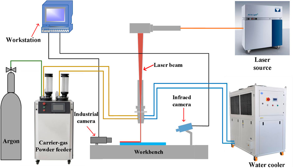
FIGURE 1. Schematic diagram of laser solid forming system.
In the present experiment, a substrate composed of 45 steel, with dimensions measuring 20 mm by 10 mm by 8 mm, was employed. To mitigate any potential temperature-related interferences resulting from multiple cladding, only a single cladding experiment was conducted for each individual substrate. Prior to commencing the experiment, the substrate surface was meticulously cleansed of impurities employing anhydrous ethanol. Fe55 powder with a particle size of 200 mesh is used as the cladding material. The chemical composition of Fe55 powder is shown in Table 1.

TABLE 1. Chemical composition of Fe55.
Temperature measurement methods for the molten pool can be classified into two categories: contact and non-contact. Contact measurements involve the use of thermocouples, which offer advantages such as affordability, simplicity in structure, and stability. However, due to the unique characteristics of Laser Solid Forming (LSF) processing, thermocouples are unable to provide real-time temperature monitoring of the molten pool. Non-contact methods, on the other hand, encompass pyrometers and infrared (IR) cameras. Pyrometers exhibit notable precision and sensitivity, but they can only provide a single temperature value representative of the entire molten pool. In this experiment, real-time monitoring of the melt pool temperature was achieved by employing an infrared camera, specifically the FLIR A615 model. The IR camera features a temperature range of 200°C–3,000°C, a resolution of 640 by 480, and a wavelength range of 7.5–14 μm. Figure 2A showcases the infrared camera used in the experiment. A specialized software system was employed to collect temperature data and thermal images at a frequency of 50 Hz, transmitting the acquired data to the workstation for further analysis. Additionally, a pyrometer was utilized to calibrate the emissivity of the molten pool, with an emissivity value of 0.29 set for the experiment. To mitigate any potential damage caused by the laser or other external factors, a filter lens was installed in front of the camera lens. Figure 2B illustrates the molten pool captured by the infrared camera.

FIGURE 2. Schematic diagram of melt pool temperature monitoring. (A) Infrared camera schematic diagram; (B) A thermal image of a melt pool captured.
To enable real-time monitoring of the out-of-focus amount, a CCD camera was positioned parallel to the part. The procedure involved the following steps: Firstly, the camera was adjusted to achieve a parallel orientation with respect to the part. Subsequently, the camera was connected to the workstation, enabling the transfer of captured images to the designated processing unit. For camera calibration, a calibration plate was employed to acquire essential camera parameters, including the rotation matrix, translation vector, distortion coefficient, and other relevant factors. Utilizing these calibrated camera parameters, the captured images were then subjected to calibration procedures to accurately measure the height of the cladding. The CCD camera system is shown in Figure 3.
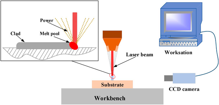
FIGURE 3. CCD camera system.
The method of converting the cladding height into off-focus amount is as follows:
In the Formula 1, S is the off-focus amount; h is the height of cladding layer; z is the z-axis lift of the laser head; n is the number of cladding layers.
Two separate sets of experiments were conducted to gather data concerning melt pool temperatures under varying process parameters. The first set of experiments was employed to establish the model, assess its feasibility, and compare the predictive accuracy of different models. The second set of experiments aimed to validate the model’s general applicability. The design of experiments is presented in detail in Table 2. In both experiments, a uniaxial scanning strategy was utilized for the fabrication of thin-walled parts, as depicted in Figure 4. Each sample consisted of fifteen layers.
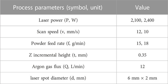
TABLE 2. Design of experiments.

FIGURE 4. Scan pattern for fabricating the thin-walled sample.
Long Short Term Memory Neural Network (LSTM) is a modified algorithm of Recurrent Neural network (RNN). The LSTM neural network adopts the mechanism of control gate, which is composed of memory cell, input gate, output gate and forgetting gate (Dupuis et al., 2022). It can keep information for a long time by updating its internal state (Zhao et al., 2021), the memory unit structure is shown in Figure 5. In the figure, X represents the input vector and h represents the output vector.
(1) First, the calculation of the information to be discarded by the forget gate. As shown in the formula:
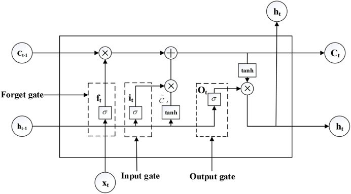
FIGURE 5. LSTM memory unit structure.
Where
(2) Determine the information that the input gate needs to save:
Then update the old memory unit state, update
Where
(3) Calculate the information to be output by the output gate:
Where
By using LSTM cyclic units, the whole network can establish long-distance temporal dependency relations. Formulas 1–6 can be simply described as:
From Figure 5, it can be seen that there are three inputs to the LSTM at time t: the input value of the network at the current time, the output value of the LSTM at the previous time and the state of the unit at the previous time. The unit state is updated by two gate structures of input gate and forgetting gate. The forgetting gate determines the previous information through the sigmoid function, as shown in Eq. 2; the input gate uses a sigmoid function to control which information should be added, as shown in Eqs 3, 4; the output of these two gates is used to update the unit state. The old unit state is multiplied by the output of the forgetting gate, plus the output of the input gate and the output of a tanh function, as shown in Eq. 5. The structure has two outputs: the output value of the current LSTM and the state of the unit at the current time, The output gate determines the information that is output from the cell state, as shown in Eqs 6, 7. In the LSTM input gates, forgetting gates and output gates work together to control the flow of information.
The PSO algorithm is an intelligent optimization algorithm that simulates the predatory behaviour of birds. When PSO solves the optimization problem, each bird in the search space represents a possible solution of the problem, and these birds are called “particles.” The characteristic information of each particle includes three types: position, velocity and fitness value, where position and velocity determine the direction and distance of the particle’s flight (Wang and Zhang, 2021). The fitness value is calculated from the fitness function and its value represents the quality of the particle (possible solution). Each iteration is not random, and each particle follows the current optimal particle to search in the solution space.
The PSO is initialized as a group of random particles (random solutions). At each iteration, the particles update their states according to two extreme values: The first value is the optimal solution found by the particle itself, called the individual optimal solution (Pbest represents its position); the other value is the optimal solution found by the whole population, called the global optimal solution (Gbest represents its position). By tracking the individual optimal solution (Pbest) and the global optimal solution (Gbest), the particles in the group constantly update their speed and position. The optimisation process in the global search space is completed by continuous iteration to find the optimal region.
The principle of the algorithm is as follows: In an m-dimensional search space, n particles form a population, the position is expressed as
Where
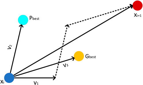
FIGURE 6. Particle state update diagram.
In the Figure 6, V1 is the direction of motion of particle i at moment t; V2 is the velocity of the particle in the direction of the individual optimal solution; V3 is the velocity in the direction of the global optimal solution. Ultimately, v is the combined effect of the velocities in all three directions, so that the particle reaches Xi+1 at the instant t+1.
The PSO process can be described as:
Step 1. Initialise the position and velocity of the particles, set the position of each particle to Pbest, calculate the fitness value of each particle and set the particle with the best fitness value to Gbest.
Step 2. Calculate the fitness value of each particle; if there is a particle with better fitness than the current Pbest, set the particle to Pbest; if there is a particle with better fitness than the current Gbest, set the particle to Gbest and update the global optimal solution.
Step 3. Update the velocity and position of each particle using Eqs 1, 2.
Step 4. If the current number of iterations reaches the specified maximum number or minimum error requirement, stop the iteration and output the optimal solution. Otherwise, go to Step 2.
The melt pool temperature during the LSF manufacturing process is a time series that is influenced by many factors and has complex nonlinearity and instabilities. In order to accurately predict the real-time molten pool temperature, this study establishes a molten pool temperature prediction model based on the LSTM algorithm that performs well in time series data prediction. Since the learning rate and the number of hidden layer units of the LSTM model have a great influence on the prediction results, the PSO algorithm is used to find the best learning rate and the most suitable number of hidden layer units to improve the prediction accuracy. In this study, the off-focus amount and real-time molten pool temperature data are used as model inputs and the output is the predicted temperature.
First, the learning rate and the number of hidden layer units are used as the optimization objects of PSO to initialize the position information of each particle. Secondly, the LSTM model is built based on the hyperparameters corresponding to the particle positions. The adaptation degree of each particle is calculated, the individual optimal solution and the global optimal solution are determined according to the adaptation degree, and the velocity and position of the particle are updated via Eqs 13, 14. Iterate until the termination condition is met and output the optimal solution. Finally, the PSO-LSTM model is built with the optimal hyperparameters. The algorithm flow is shown in Figure 7.
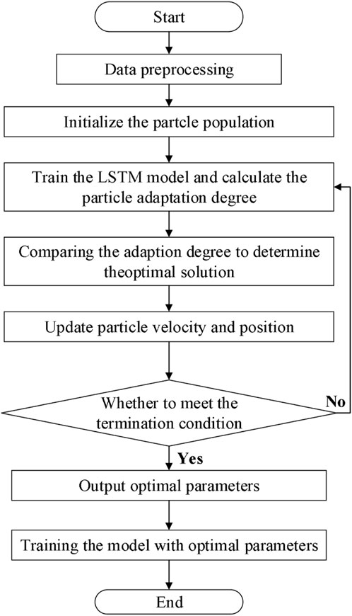
FIGURE 7. PSO-LSTM process diagram.
The PSO-LSTM process can be described as:
Step 1. Data preprocessing the experimental data is not a unified gauges, and large differences in values have a large effect on the prediction results, so the data are normalised. This is shown in Eq. 5:
Where
Divide the normalized data into a training set, a test set and a validation set.
Step 2. Initialize the PSO algorithm with the learning rate and the number of hidden layer units in the LSTM model as optimization objects.
Step 3. The LSTM model is constructed based on the hyperparameters represented by the particles, the model is trained using the training data, and the validation data is put into the trained model for prediction. The fitness value is calculated for each particle and the fitness function f is defined as:
Where
Step 4. Comparing the particle adaptation degree to determine the individual optimal solution Pbest and the global optimal solution Gbest.
Step 5. Update the velocity and position of the particle according to Eqs 1, 2.
Step 6. Determine whether the termination conditions are met. If the termination condition is met, the optimum parameter value is output; if the termination condition is not met, return to Step 3.
Step 7. The LSTM model is constructed using the optimal learning rate and the number of hidden layer units.
Figure 2B shows an image of the melt pool taken during the experiment. In this study, the peak temperature within the melt pool boundary was used to measure the melt pool temperature. Figure 8 shows the melt pool temperature measured during Experiment 1, where the process parameters were laser power of 2,100 W, scan speed of 12 mm/s and powder feed rate of 15 g/min. During the experiment, the dwell time between adjacent layers was kept constant at 6 s. When we focus only on the melt pool temperature within each layer, the temperature collected during the dwell time between adjacent layers is removed from the modelling process. Figure 8A shows the temperature data of the 15 layers during the manufacturing process, from the graph it can be visually observed that there are temperature fluctuations in each layer. The temperature fluctuation is caused by the varying localized thermal histories. The energy absorbed by the melt pool changes continuously over the course of the long processing time due to fluctuations in the amount of off-focus and other factors. The inconsistent energy input further influences the melt pool size and geometry, which determines the local temperature and cooling rate (Pinkerton, 2010). In order to observe the temperature fluctuation more clearly, Figure 8B shows the temperature data of 1, 15 layers.
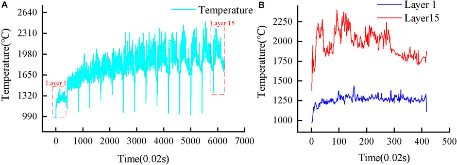
FIGURE 8. Experiment 1 Melt pool temperature profile. (A) Measured melt pool temperature of experiment 1; (B) Measured melt pool temperature of layer 1, 15 in (A).
From the melt pool temperature variation curve, it can be seen that in layers 1 to 9, the melt pool temperature gradually increases with the number of layers due to the heat accumulation effect; once the number of layers reaches 10 or more, we can observe a similar periodicity of melt pool temperature variations between adjacent layers. The reason for this phenomena is because as the deposited layers accumulate to a certain height, the volume of the material melting increases, the material’s heat capacity also increases, and the absorbed heat is distributed throughout a larger volume of the material. At the same time, heat conduction within the material increases gradually. Heat conduction is the process of transferring heat from a high temperature zone to a low temperature zone. When heat is rapidly transferred within a material, the rate of local temperature change is also slowed. As a result, when a certain height is reached, heat generation and transport approach a dynamic balance, and the overall trend of melt pool temperature fluctuations has a cyclical nature.
The PSO-LSTM model consists of one input layer, two LSTM layers and one output layer. The model training process is optimised using the Adma algorithm and the number of iterations is set to 250. The hyperparameters in the LSTM model are set as follows: the learning rate is set in the range (0.001, 0.01) and the number of hidden layer units is set in the range (10, 30). The number of particles in the swarm is set to 50, the maximum number of iterations is 400, the velocity inertia weight is set to 0.85 and the sum of the acceleration factors is 2.
In order to evaluate the prediction performance of the model scientifically and objectively, this paper uses root mean square error (RMSE), mean absolute error (MAE) and coefficient of determination (R2) as evaluation indicators to quantitatively assess the accuracy of the prediction model. These error metrics are defined as:
The notations
Firstly, the melt pool temperature data obtained from Experiment 1 was divided into a training set, a validation set, and a test set, where the last 100 sampling points were used as test data, 80% of the remaining data were used as training data, and 20% as validation data. The LSTM, PSO-LSTM, and ridge regression models were then used for temperature prediction, respectively. Using ridge regression as the control group, the prediction results are shown in Figure 9: the red curve represents the true temperature values, and the blue curve represents the predicted temperature values.
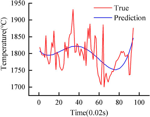
FIGURE 9. Ridge regression prediction results.
The LSTM and PSO-LSTM prediction results are shown in Figure 10. The prediction results show that the ridge regression model has the worst prediction accuracy. This suggests that machine learning algorithms with low flexibility are not as capable of modeling non-linear relationships for complex time-series data and cannot achieve accurate predictions; The prediction curve of the PSO-LSTM model proposed in this study is closer to the real melt pool temperature curve, especially at large temperature fluctuations, and the prediction effect of the PSO-LSTM is better than that of other models.
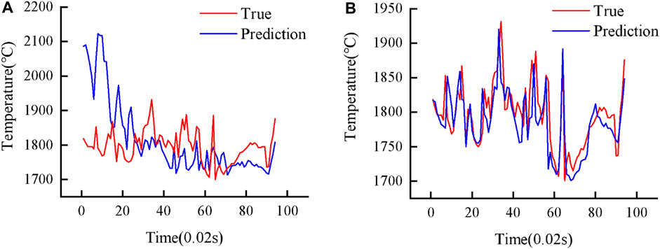
FIGURE 10. Comparison of prediction results of different models. (A) LSTM prediction results; (B) PSO-LSTM prediction results.
To further validate the predictive performance of the model, Table 3 shows the results of the evaluation metrics calculated for each predictive model. The RMSE and MAE evaluation indicators of the PSO-LSTM model are lower than the other two models; In the coefficient of determination (R2) evaluation criteria, the PSO-LSTM model calculates results closer to 1 than other prediction models. The results show that the prediction accuracy of the PSO-LSTM model is higher than the prediction accuracy of other models.

TABLE 3. Evaluation results of each model.
To further validate the accuracy, stability and general applicability of the PSO-LSTM model, three models were used to predict the melt pool temperature for Experiment 2. The process parameters for experiment 2 are as follows: laser power 2,400 w, scanning speed 10 mm/s and powder feed rate 18 g/min. Again using Ridge regression as a reference, the predicted results are shown in Figure 11.
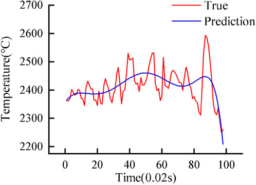
FIGURE 11. Predicted melt pool temperature of experiment 1 (p = 2,400, v = 10, f = 18).
The predicted melt pool temperatures for the LSTM and PSO-LSTM are shown in Figure 12. The results show that PSO-LSTM has the best prediction performance, and Ridge regression has the worst.
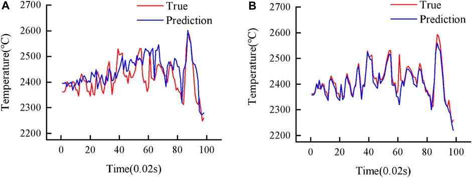
FIGURE 12. Comparison of prediction results of different models. (A) LSTM predicts melt pool temperature; (B) PSO-LSTM predicts melt pool temperature.
Table 4 shows the evaluation metrics for each model for Experiment 2. Comparing the PSO-LSTM model to the other two models, the MSE and MAE assessment indices are lower for the PSO-LSTM model; the PSO-LSTM model generates outcomes that are closer to 1 than other prediction models in terms of the coefficient of determination (R2) assessment criterion. This shows that PSO-LSTM has the best prediction performance.

TABLE 4. Experiment 2(p = 2,400 w, v = 10 mm/s, f = 18 g/min) evaluation results for each model.
In order to achieve accurate prediction of real-time melt pool temperature, a PSO-LSTM based melt pool temperature prediction method is proposed in this paper. Based on Ridge regression, LSTM, and PSO-LSTM methods, three melt pool temperature prediction models were created. Perform different experiments to validate and train the models. The following conclusions were obtained:
1) A PSO-LSTM based melt pool temperature prediction model was developed using the PSO algorithm to optimize the learning rate and the number of hidden layer units of the LSTM model. The results show that the PSO-LSTM can accurately predict real-time melt pool temperatures, and in particular predicts temperature trends at sharp temperature fluctuations better than other models.
2) Based on the experimental results, a comparison of the predictive performance of PSO-LSTM, LSTM models and ridge regression models is performed. The PSO-LSTM model has lower values of MAE and RMSE evaluation indicators than other models, and the coefficient of determination is closer to 1. The PSO-LSTM model has better predictive performance than other models and can predict the melt pool temperature more accurately, providing guidance for real-time regulation of the melt pool temperature.
3) In this study, prediction of molten pool temperature in laser solid forming were carried out, with high agreement between predicted and real temperatures. However, other performance index of cladding layer such as laser cladding height and tensile strength need to be modeled and predicted to guide the application of LSF process in the future study. In addition to the machine algorithms used in this paper, more advanced machine learning algorithms can be used to build optimal prediction models.
The original contributions presented in the study are included in the article/Supplementary Material, further inquiries can be directed to the corresponding authors.
Conceptualization, JW and JX; methodology, JW and JX; validation, JW, JX, and YL; formal analysis, JX; investigation, YL and JP; resources, JW; data curation, FY, JP, and XM; writing—original draft preparation, JX; writing—review and editing, JW; visualization, JX; supervision, TX; project administration, JW; funding acquisition, JW, and JP. All authors contributed to the article and approved the submitted version.
This research was funded by the Joint Funds of Science Research and development Program in Henan Province (222103810039 and 222103810030), Henan Province Science and Technology key issues (222102220073), Key Scientific Research Project of Colleges and Universities in Henan Province (22A460014).
The authors declare that the research was conducted in the absence of any commercial or financial relationships that could be construed as a potential conflict of interest.
All claims expressed in this article are solely those of the authors and do not necessarily represent those of their affiliated organizations, or those of the publisher, the editors and the reviewers. Any product that may be evaluated in this article, or claim that may be made by its manufacturer, is not guaranteed or endorsed by the publisher.
Bhandari, H. N., Rimal, B., Pokhrel, N. R., Rimal, R., and Dahal, K. R. (2022). LSTM-SDM: An integrated framework of LSTM implementation for sequential data modeling. Softw. Impacts 14.doi:100396
Bhatnagar, S., Mullick, S., and Gopinath, M. (2021). A lumped parametric analytical model for predicting molten pool temperature and clad geometry in pre-placed powder laser cladding. Optik 247.doi:168015
Dupuis, A., Dadouchi, C., and Agard, B. (2022). Tacit knowledge in production sequencing: A Seq2Seq-LSTM approach. IFAC-PapersOnLine 55, 1600–1605.
Fathi, A., Toyserkani, E., Khajepour, A., and Durali, M. (2006). Prediction of melt pool depth and dilution in laser powder deposition. J. Phys. D Appl. Phys. 39, 2613.
Gao, J., Wang, C., Hao, Y., Wang, X., Zhao, K., and Ding, X. (2022). Prediction of molten pool temperature and processing quality in laser metal deposition based on back propagation neural network algorithm. Opt. Laser Technol. 155.doi:108363
Gao, J., Wu, C., Hao, Y., Xu, X., and Guo, L. (2020). Numerical simulation and experimental investigation on three-dimensional modelling of single-track geometry and temperature evolution by laser cladding. Opt. Laser Technol. 129.doi:106287
Huang, C., Liang, R., Liu, F., Yang, H., and Lin, X. (2022). Effect of dimensionless heat input during laser solid forming of high-strength steel. J. Mater. Sci. Technol. 99, 127–137.
Izumi, M., and Iwai, T. (2020). Hybrid model of linked and unlinked random PSO models. Artif. Life Robotics 25, 258–263.
Khanzadeh, M., Chowdhury, S., Tschopp, M. A., Doude, H. R., Marufuzzaman, M., and Bian, L. (2019). In-situ monitoring of melt pool images for porosity prediction in directed energy deposition processes. IISE Trans. 51, 437–455.
Kulchin, Y., Gribova, V., Timchenko, V., Basakin, A., Nikiforov, P., Yatsko, D., et al. (2022). Melt pool temperature control in laser additive process. Bull. Russ. Acad. Sci. Phys. 86, S108–S113.
Meng, L., Mcwilliams, B., Jarosinski, W., Park, H.-Y., Jung, Y.-G., Lee, J., et al. (2020). Machine learning in additive manufacturing: A review. Jom 72, 2363–2377.
Mozaffar, M., Paul, A., Al-Bahrani, R., Wolff, S., Choudhary, A., Agrawal, A., et al. (2018). Data-driven prediction of the high-dimensional thermal history in directed energy deposition processes via recurrent neural networks. Manuf. Lett. 18, 35–39.
Pinkerton, A. (2010). “Laser direct metal deposition: Theory and applications in manufacturing and maintenance,” in Advances in laser materials processing (Elsevier), 461–491.
Shao, Y., Xu, P., and Tian, J. (2021). Numerical simulation of the temperature and stress fields in Fe-based alloy coatings produced by wide-band laser cladding. Metal Sci. Heat Treat. 63, 327–333.
Wang, D., Liu, G., Prasad, B. D., Xiao, T., and Yang, Y. (2023). FFSCore-LSTM: An enhanced LSTM-based camera relocalization networks via front feature smoothing core. Measurement 210.doi:112542
Wang, H., and Zhang, H. (2021). Visual mechanism characteristics of static painting based on PSO-BP neural network. Comput. Intell. Neurosci. 2021.
Wu, Yu., Ma, Pengzhao., and Bai, Wenqian. (2021). Numerical simulation of temperature field and stress field in 316l/aisi304 laser cladding with different scanning strategies. Chin. J. Lasers 48, 18–29.
Xiao, L., Peng, Z., Zhao, X., Tu, X., Cai, Z., Zhong, Q., et al. (2022). Microstructure and mechanical properties of crack-free Ni-based GH3536 superalloy fabricated by laser solid forming. J. Alloys Compd. 921.doi:165950
Yang, H.-O., Zhang, S.-Y., Lin, X., Hu, Y.-L., and Huang, W.-D. (2021). Influence of processing parameters on deposition characteristics of Inconel 625 superalloy fabricated by laser solid forming. J. Central South Univ. 28, 1003–1014.
Yuming, H., Jiaohong, L., Zhenguo, M., Bing, T., Keqi, Z., and Jianyong, Z. (2023). On combined PSO-SVM models in fault prediction of relay protection equipment. Circuits, Syst. Signal Process. 42, 875–891.
Zhang, Z., Liu, Z., and Wu, D. (2021). Prediction of melt pool temperature in directed energy deposition using machine learning. Addit. Manuf. 37.doi:101692
Zhao, J., Lin, J., Liang, S., and Wang, M. (2021). Sentimental prediction model of personality based on CNN-LSTM in a social media environment. J. Intelligent Fuzzy Syst. 40, 3097–3106.
Zhao, Yu-hui., Yao, Chao., and Wang, Zhi-guo (2020). Research on test and prediction method of molten pool by laser additive maufacturing. Vacuum 57, 76–82.
Keywords: laser solid forming (LSF), molten pool temperature, predictive modelling, particle swarm optimization, long short-term memory neural network
Citation: Wang J, Xu J, Lu Y, Xie T, Peng J, Yang F and Ma X (2023) Prediction of molten pool temperature in laser solid forming based on PSO-LSTM. Front. Mater. 10:1218222. doi: 10.3389/fmats.2023.1218222
Received: 06 May 2023; Accepted: 19 May 2023;
Published: 31 May 2023.
Edited by:
Kun Li, Chongqing University, ChinaReviewed by:
Hao Yi, Chongqing University, ChinaCopyright © 2023 Wang, Xu, Lu, Xie, Peng, Yang and Ma. This is an open-access article distributed under the terms of the Creative Commons Attribution License (CC BY). The use, distribution or reproduction in other forums is permitted, provided the original author(s) and the copyright owner(s) are credited and that the original publication in this journal is cited, in accordance with accepted academic practice. No use, distribution or reproduction is permitted which does not comply with these terms.
*Correspondence: Junhua Wang, d2FuZ2poQGhhdXN0LmVkdS5jbg==; Tancheng Xie, eGlldGNAaGF1c3QuZWR1LmNu
Disclaimer: All claims expressed in this article are solely those of the authors and do not necessarily represent those of their affiliated organizations, or those of the publisher, the editors and the reviewers. Any product that may be evaluated in this article or claim that may be made by its manufacturer is not guaranteed or endorsed by the publisher.
Research integrity at Frontiers
Learn more about the work of our research integrity team to safeguard the quality of each article we publish.