 Gang Lv
 Haoliang Lv2*
94% of researchers rate our articles as excellent or good
Learn more about the work of our research integrity team to safeguard the quality of each article we publish.
Find out more
ORIGINAL RESEARCH article
Front. Mater., 18 May 2023
Sec. Mechanics of Materials
Volume 10 - 2023 | https://doi.org/10.3389/fmats.2023.1188411
At present, research on the loading simulation test bench for overloaded vehicles is mostly limited to the realization of loading simulation under the condition of straight line driving of the vehicle. When simulating the whole vehicle load under straight line driving condition, only accurate road load and inertial load can be obtained to achieve accurate load simulation, and the inertial load required to be simulated by each side device is half of the whole vehicle inertial load. However, straight line driving is only the most ideal driving. The real driving conditions (including ground conditions) of the vehicle are usually composed of steering, longitudinal slope, lateral slope and different ground adhesion coefficients. Therefore, the loads borne by the two independent load simulation systems located on both sides of the vehicle may be different during the load simulation process. In addition, the frequency characteristics of the loads to be simulated by the same side load simulation device at different time sequences may also be different. This paper studies the dynamics modeling, load distribution and error compensation in the whole vehicle load simulation process in order to achieve accurate crawler vehicle load simulation from three aspects.
In the actual driving process of tracked vehicles, the vehicle and its driven and transmission parts are affected by external factors such as inertia load, wind resistance, slope resistance, etc., in real time. These influencing factors are constantly changing in an unordered manner as the vehicle travels. In the bench test, since the test piece is fixed and immovable, these factors cannot be reflected. Therefore, the running resistance of the test piece in the bench test is different from the real situation. In order to ensure the authenticity and accuracy of the load simulation on the test bench, compensation loading needs to be applied to the test pieces running on the test bench, and the core technology for achieving compensation loading is the load simulation technology (Fajri et al., 2013; Yang et al., 2013; Takeda et al., 2014).
Accurate load simulation is premised on having an accurate vehicle load model. The load on the drive system during the vehicle’s journey can be divided into road load and inertial load. The road load of the vehicle is formed by the gravity of the vehicle, the driving conditions of the vehicle, the ground conditions, etc. In the discussion of road load, the changes in the load on the left and right wheels under different driving conditions need to be considered. For tracked vehicles, the distribution of the load on the ground where the track is in contact needs to be taken into consideration.
In reference Xingguo et al. (2011), dynamics analysis and discussion of tracked vehicles were conducted by using multi-body dynamics software, and vehicle models applicable to different roads were obtained by modeling and simulation based on different road models. This provides a theoretical basis for the performance analysis of the whole vehicle and vehicle components. In reference Bai et al. (2017) and others, in order to study the dynamic load characteristics of the multi-axis vehicle powertrain system, a dynamic simulation model of the multi-axis vehicle powertrain system was established. The author established the dynamic simulation model of the transmission system including the hydraulic torque converter, clutch, differential, differential, main reducer, wheel side reducer, etc., and established the dynamic simulation model of the multi-axis vehicle powertrain system in Simulink. The comparison results of simulation and experimental data show that the model can effectively simulate the dynamic load characteristics and speed characteristics. The inertial load is the load formed by the inertia of the whole vehicle during the acceleration process. When establishing a wheeled vehicle dynamic model using traditional methods, the coefficients of the rotating components (such as wheels and transmission systems) and the equivalent inertia of the output shaft are estimated to calculate the body inertia, which is then equivalent to the output shaft (Kim et al., 2003; Fu et al., 2009; Wang et al., 2018). In the modeling process of general light-load vehicles, the kinetic energy of the rotating components and the slip rate between the vehicle and the ground are basically ignored. Due to the ratio of the mass of the rotating part to the total mass of the wheeled vehicle being very small, the estimation error of the equivalent mass is very small.
In reference Ott et al. (2021), a multibody system was used, which consists of five bodies. By applying methods of multibody modelling the generalized equations of motion were generated. To include the behavior within the contact point between road and vehicle a simplified tire models was added. The model was simulated numerically to investigate different load states of the vehicle, by applying constant steering stimuli and variable velocities. In reference ChenZhouWang et al. (2019), in order to study the braking performance of electric tracked vehicles, the vehicle ground contact state under straight driving conditions was analyzed, a vehicle slip rate model was established, and fuzzy control algorithm was used to simulate the synchronous load on both sides of the vehicle. In reference Jiang et al. (2022), a three-degree-of-freedom vehicle dynamics model is established accurately, a rollover evaluation index and a safety threshold are selected quickly, and the working principle and detailed control scheme of the motor speed control strategy are given. In order to achieve stable control of vehicle driving in a straight direction, reference (Lv et al., 2019) proposed a 2-degree-of-freedom (2-DOF) control method combined with a disturbance observer to solve the stability problem of the system. The test results show that the system has a high load simulation accuracy under various load simulation tests.
Heavy-duty vehicles have different modeling of equivalent inertia due to their special structure (Huh et al., 2001; Zou et al., 2016). Taking tracked vehicles as an example, the rotating parts of tracked vehicles include parts with a large proportion of vehicle weight, such as tracks (Wang and Sun, 2014). If the same calculation method as wheeled vehicles is adopted, a larger error will be produced. Therefore, in the process of heavy-duty vehicle load simulation, different forms of modeling must be carried out for different vehicles to ensure the accuracy of the model.
According to the current research progress, there are two problems in the research of vehicle load:
1) When establishing the road load model of the vehicle, the driving condition is relatively simple, which cannot accurately reflect the load and its distribution of the vehicle under general driving conditions;
2) Lack of in-depth research on the equivalent inertia of tracked vehicles, and lack of research on the distribution of equivalent inertia of ground slip rate, left and right driving wheels in the modeling process.
To address the above issues, this article establishes a dynamic model for the complex driving process of the entire vehicle, considers the load distribution of the vehicle under various operating conditions, and establishes the accurate equivalent inertia of the vehicle during the load simulation process. The inertia torque formula is used to achieve the load simulation of the vehicle. To improve the load simulation accuracy of the vehicle, a form of cross coupling error compensation is proposed to reduce the error of the simulation device.
The road load on the whole vehicle during its running process is derived from the energy loss of wheel/track ground friction, slope resistance and resistance generated by ground deformation. Due to the interaction of various forces such as slope resistance, steering resistance and centrifugal force during the running process of the vehicle, the road load on the vehicle is different in different running states. This section takes tracked vehicles as an example to analyze their kinematics and dynamics, and explore the road load of the vehicle under different driving conditions.
In the process of vehicle load simulation, the test bench needs to reproduce the actual working conditions of the vehicle on the actual road surface, that is, the bench needs to respond to both the torque output of the vehicle’s driving system and the speed output of the vehicle (Nam, 2001). It can be seen that the load simulated by the motor in the load simulation system is determined by the output of the vehicle’s driving wheel. The principle of load simulation is shown in Figure 1:
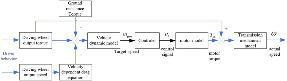
FIGURE 1. Load simulation schematic diagram.
The tested vehicle in Figure 1 is controlled by the driver’s behavior, outputting speed and torque. After the speed and torque signals are obtained by the sensor, the target speed of the system is obtained through the superposition with the resistance torque and the vehicle dynamics model. The target speed is converted into an electrical signal, which is then converted into the motor output torque through the controller and motor transfer function model. The output torque of the motor and the output torque of the vehicle’s driving wheel jointly act on the transmission mechanism, allowing the transmission mechanism to output the actual speed to achieve load simulation of the entire vehicle.
As shown in Figure 1, in order to accurately reproduce the rotational speed output of the entire vehicle, it is necessary to obtain the accurate equivalent inertia of the entire vehicle equivalent to the driving wheel. According to the formula for balancing the driving force of the entire vehicle, assuming that the torque output from the driving system to the driving wheel under a certain working condition is
In the formula,
During the actual road driving process of a vehicle, the body motion is divided into two parts: translational and rotational. Assuming that the translational part of the vehicle is a rigid block with a mass of
At this point, the relationship between
Where
During the driving process of the vehicle, the inertia resistance and road resistance experienced by the entire vehicle are transmitted to the vehicle drive system in the form of loads through the wheels. Assuming that the effective working radius of the wheels is R, the torque T on the half axle is:
Substitute Eq. 3 into Eq. 4 and perform Laplace transformation to obtain:
Where
Then
According to Eq. 5 and Eq. 6, from the perspective of discrete domain analysis, with known equivalent inertia
Meanwhile, the load simulation system consists of a load motor and a mechanical transmission system. From the perspective of force acting on the test bench, the torque balance equation of the bench is:
Wherein,
When the vehicle carries out the load simulation test according to the method in Figure 1, it can be seen that
According to the above equation, in order to accurately achieve the load simulation function of the platform, it is necessary to obtain an accurate road load model
Currently, the kinematics and dynamics of the whole vehicle of tracked vehicles are usually studied in terms of steering motion in the horizontal plane or straight line motion on a slope (Yalla et al., 2007; Janarthanan et al., 2011). This type of working condition can only represent part of the working conditions during the vehicle’s travel. In order to comprehensively study the kinematics and dynamics of the vehicle under the load working condition, this section establishes the vehicle motion coordinate system shown in Figure 2A. Assuming that the tracked vehicle is traveling on a slope with an inclination angle of
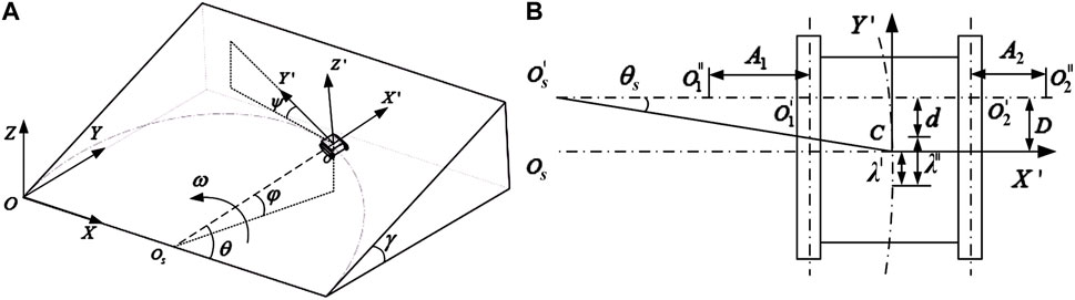
FIGURE 2. (A) The instantaneous posture of the vehicle when turning on a certain slope; (B) Kinematic analysis of
At this moment, according to Figure 2A, the instantaneous side tilt angle
The instantaneous pitch angle
The components of the weight of the vehicle in the
Analysis of the motion of the vehicle in the
The traction speed of the center line of the track on both the inside and outside when the tracked vehicle is turning is:
Where B is the width of the vehicle;
In the process of motion analysis, assuming that the ground contact of the tracks is all concentrated on the center line
The slip rate of the tracks on both sides inside and outside can be expressed by the following equation:
According to Figure 2B:
Further deducted, it can be obtained as:
Analysis of the forces on the vehicle in the
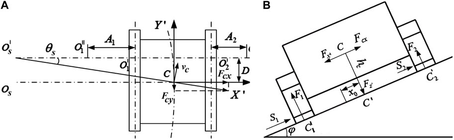
FIGURE 3. (A) Dynamics analysis of
In the
According to the above figure, the ground reaction forces of the left and right tracks can be obtained by calculating the moment at points
Therefore, the center of the ground support reaction along the
In the
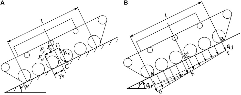
FIGURE 4. (A) Whole vehicle plane force analysis; (B) Analysis of normal load of track ground contact.
When a tracked vehicle turns on a horizontal plane, the combined force of the ground reaction force and the pressure center of the track contacting the ground coincide. When the vehicle is running on a slope, the ground counteraction force provided to the track can be decomposed into the vertical support force
Then it is easy to get the expression of the bias distance
Due to the offset of the normal force center of the ground, the normal load of the track contacting the ground changes from rectangular to trapezoidal at this time. The unit length normal load at the front end is
According to Figure 4B,
Then it can be obtained:
Further it can be obtained:
Due to the longitudinal component
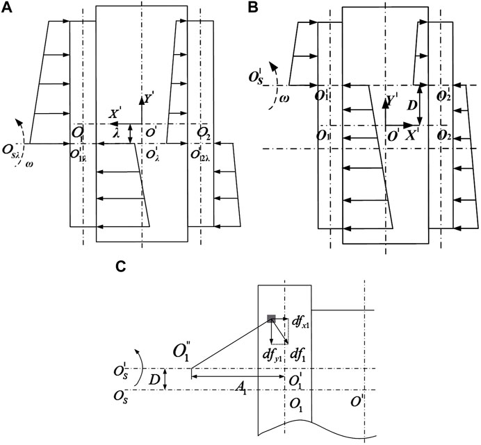
FIGURE 5. (A) Vehicle lateral force model without considering slip and yaw; (B) Vehicle lateral force model considering slip and yaw; (C) Analysis of the force on the inner track contacting the ground during the steering process.
A force analysis model of the ground contact element of the track has been established in the
It can be obtained that the force on each contact ground element in the
In the equation,
In the equation,
Further derivation of Eq. 27 can obtain the friction resistance components in the
According to D'Alembert’s principle, the force balance equation of the vehicle can be obtained in the relative coordinate system
In the equation,
In the equation,
Substituting Eq. 29 into Eq. 30, it can be seen that the equation set listed has hidden unknown motion parameters, and there is a coupling relationship between the parameters, so the iterative method is used to solve it.
To study the road load of tracked vehicles under different driving conditions, Eq. 30 is applied to perform kinematic/dynamic simulations on the tracked vehicles and the parameters of the viscous soil conditions by using the MATLAB programming environment.
When the weight of the vehicle is 38 tons, the width of the vehicle is 3.5 m, the radius of the driving wheel is 0.286 m, the height of the center of mass is 1.25 m, the track length is 5 m, and the track width is 0.4 m, then we have:
Assuming that the vehicle speed remains at 3 m/s and the steering radius remains at 30 m, the kinematic states of the vehicle are shown in Figures 6A–E as the inclination angle
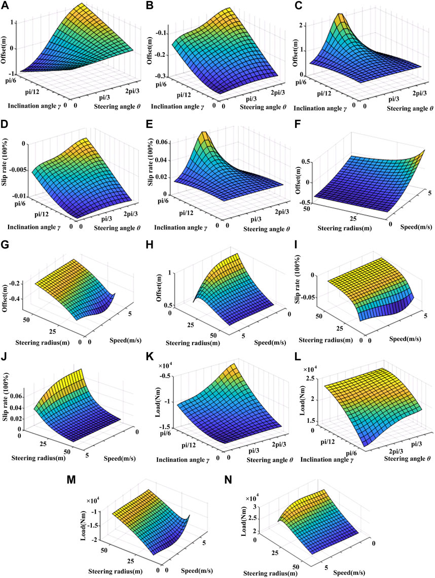
FIGURE 6. (A) Longitudinal offset of the turning center under different inclination angles and steering angles; (B) Instantaneous lateral offset of the turning center of the inner trackunder different inclination angles and steering angles; (C) Instantaneous lateral offset of the turning center of the outer trackunder different inclination angles and steering angles; (D) Ground slip ratio of the inner trackunder different inclination angles and steering angles; (E) Ground slip ratio of the outer trackunder different inclination angles and steering angles; (F) Longitudinal offset of the steering center under different steering radii and speeds; (G) Inner steering center lateral offsetunder different speeds and steering radii; (H) Outer steering center lateral offsetunder different speeds and steering radii; (I) Ground slip ratio of the inner trackunder different speeds and steering radii; (J) Ground slip ratio of the outer trackunder different speeds and steering radii; (K) Inner drive wheel loadunder different inclination angles and steering angles conditions; (L) Outer drive wheel loadunder different inclination angles and steering angles conditions; (M) Inner drive wheel loadunder different speeds and steering radii conditions; (N) Outer drive wheel loadunder different speeds and steering radii conditions.
From Figure 6A, it can be seen that when the vehicle is in the
Figures 6B, C show the lateral offset curve of the instantaneous steering center of the two tracks. For the inner track, the lateral offset of the instantaneous center of speed increases nonlinearly with the increase of the steering angle and inclination angle. For the outer track, when
By comparing Figures 6B–E, it can be seen that the ground slip ratio of the two tracks and the distribution curve of the lateral offset of the turning center of the tracks have a similar trend. The main reason for this can be obtained by analyzing Eq. 16 and Eq. 17. The combination of the two equations shows that the ground slip ratio of the track is linearly positively correlated with the lateral offset of the steering center. Therefore, the lateral offset of the steering center is the main factor affecting the ground slip ratio of the tracks.
Assuming the vehicle is driving on a surface with a inclination angle of
From Figure 6F, it can be seen that at different steering radii, as the vehicle speed increases, the longitudinal offset of the vehicle’s steering center moves forward, because the vehicle needs to move the steering center forward to match the gradually increasing centrifugal force, which conforms to the laws of vehicle kinematics.
The influence of vehicle speed and steering radius on the lateral offset of the instantaneous steering center of the tracks is shown in Figures 6G, H. It can be seen from the figure that the absolute value of the lateral offset of the instantaneous steering center of both tracks is negatively correlated with the vehicle steering radius, and when the vehicle steering radius is large, the lateral offset of the steering center is not sensitive to changes in vehicle speed. This is because when the vehicle is making a large-radius turn, the difference in load between the two tracks decreases, and when the vehicle’s steering radius approaches infinity, the vehicle travels in a straight line.
Figures 6I, J shows the variation curves of instantaneous track slip ratios under different vehicle speeds and steering radii. As can be seen from Figure 6I, if the steering radius remains unchanged, the vehicle speed has a small effect on the slip ratio, and the slip ratio of the inner track increases gradually as the steering radius decreases. By comparing Figures 6I, J, it can be found that the vehicle speed only has a significant effect on the slip ratio under low steering radius conditions. This is because as the steering radius of the vehicle increases, the trajectory of the entire vehicle tends to be more straight-line movement. This phenomenon conforms to the laws of vehicle motion.
As shown in Figures 6K, L, it can be seen that during vehicle operation, the load on the inner driving wheel is positively correlated with the inclination angle and steering angle, while it is negatively correlated with the load on the outer driving wheel. This is mainly because as the inclination angle and steering angle of the vehicle increase, the center of gravity of the vehicle gradually shifts towards the inner track, causing an increase in the vertical load on the inner track.
The impact of vehicle speed and steering radius on the load of the two driving wheels is shown in Figures 6M, N. As shown in Figures 6M, N, when the steering radius of the vehicle increases, the vehicle tends to travel in a straight line, and the absolute value of the load on both sides of the wheels gradually decreases. When the steering radius of the vehicle is constant and the speed increases, due to the change of centrifugal force, the absolute value of the load on both sides of the wheels decreases in a parabolic shape. Moreover, when the steering radius of the vehicle increases, the impact of speed on the load of the vehicle gradually decreases.
In actual driving, the load on the two sides of a heavy-duty vehicle is not the same and changes dynamically due to the vehicle’s own driving and transmission system characteristics as well as the external road environment. For the load simulation system, the load motor on one side applies a load to the tested vehicle, which is also affected by the corresponding output torque of the output shaft and the simulated ground environment. Therefore, one of the key points to achieve accurate whole vehicle load simulation is to dynamically allocate the load and inertia required to be simulated to the load simulation motors corresponding to each driving axle through dynamic allocation, and each load simulation motor then implements the vehicle load simulation using the single axle load simulation method (Bekker, 1960).
For simple load simulations, such as straight driving, the simplest method is to evenly distribute the load and inertia of the tested vehicle to each axle, and the vehicle’s speed can also be directly obtained based on the speed of each axle. However, straight driving is just a special case of vehicle operation. During acceleration, braking, turning and other actions, different load distributions on both sides, turning radii, and driving speeds will occur. Therefore, in simulating the entire vehicle, evenly distributing the road load and inertial load on each side of the vehicle will inevitably result in accuracy errors in load simulation, and it is necessary to correct it by properly distributing the vehicle load.
During the load simulation process, the simulated load of the load simulation system is obtained by considering the vehicle’s dynamic model and the external forces acting on the vehicle. When the external environment of the vehicle changes, the load on the left and right wheels also changes accordingly, and this load change is reflected on the test bench in the form of changes in the road load and inertia load. In the previous section, this paper obtained the vehicle’s road load model. In this section, the allocation of inertia load is discussed in depth.
For vehicle driving, steering is a universal situation that can be used to describe the driving state of the vehicle in different environments and conditions. Straight-line driving of the vehicle is a special case of the vehicle’s steering driving, which can be described as the driving condition when the steering radius
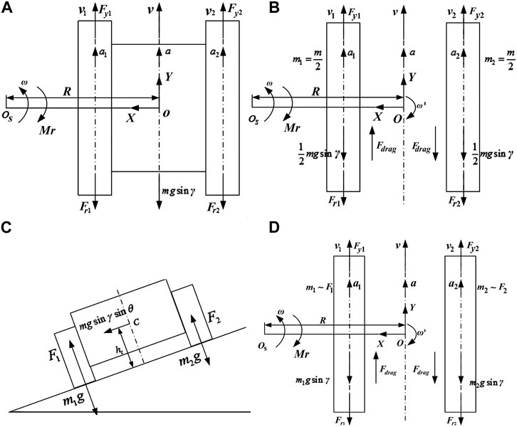
FIGURE 7. (A) The force analysis of a stable condition with the same load on both sides; (B) The force analysis of an unstable condition with the same load on both sides; (C) Analysis of forces with different loads on both sides; (D) Analysis of forces with different loads on both sides on unsteady-state condition.
In the figure, let the instantaneous velocity direction of the vehicle be the Y direction and the direction of the line connecting the vehicle’s center of mass and the turning center be the X direction. Since the load on both sides is the same and the velocity is the same, it can be deduced that the driving forces of the left and right tracks are
It can be further deduced that
When the vehicle is traveling in a straight line on a horizontal surface or during low-speed turning, assuming that at a certain moment, one side of the ground contact surface slips. At this time, the coefficient of adhesion of the ground changes, and the single-side ground adhesion force cannot provide sufficient driving force. In order to investigate the load situation of the driving wheel under the conditions of the entire vehicle and side-by-side, the entire vehicle is divided into two parts, left and right, and these two parts are connected in the Y direction through a pair of equal and opposite original forces
Based on the above figure, in the vehicle coordinate system, the second law of Newton in the Y direction and the steering direction are as follows:
At this point, it can be reasonably assumed that the vehicle is designed such that
In the equation,
According to Eqs. 33–37, We can get the result:
Where
That is:
When
This shows that under certain driving conditions and ground adhesion conditions, the equivalent inertia of the vehicle may be distributed unequally. When the condition in Eq. 39 is satisfied, for a certain active wheel, the transfer force
When the vehicle is moving on a slope or when the position of the vehicle’s center of gravity changes, the supporting forces acting on the wheels/tracks on both sides of the vehicle by the ground are not equal, as shown in Figure 7C. According to Eq. 38, it can be known that when the acceleration on both sides of the vehicle satisfies certain conditions and plus
The calculation based on Eq. 19 suggests that the equivalent masses acting on the wheels on both sides of the vehicle are:
After calculation of Equivalent inertia, we have:
During the vehicle’s operation, its behavior is affected by the driver’s driving behavior, which belongs to a pseudo-random working condition. At the same time, the ground conditions for vehicle operation are influenced by soil composition, water content, and terrain, resulting in different ground adhesion forces on both sides of the vehicle. Therefore, when considering the equivalent inertia of both sides, not only the distribution of vertical loads but also the variation of the internal transfer force
In Figure 7D,
According to Eq. 38, We can get the result:
Which also means:
When
In the same way, the equivalent inertia on both sides can be obtained as:
Through the study of vehicle equivalent inertia distribution, this section establishes a model of equivalent inertia distribution as described in Eq. 32, Eq. 41, Eq. 43, and Eq. 48. By studying the inertial load, errors in load simulation caused by uneven distribution of inertial load are avoided.
Through the derivation in Section 4.2, the inertia load model of the whole vehicle under different driving conditions can be obtained. Based on these models, to further obtain the target speed of the vehicle, it is necessary to know the current driving wheel speed
During vehicle operation, the steering wheel reflects the driver’s steering demand. When the steering wheel angle
The relationship between the vehicle linear velocity
Therefore, through the vehicle’s steering wheel angle signal, the driving wheel speed signal, and the current ground slip ratio, the target steering radius of the vehicle at the next moment can be known. By introducing these parameters into the vehicle dynamics model and combining them with the vehicle equivalent inertia model, the control model of the whole vehicle load simulation can be obtained, as shown in Figure 8.
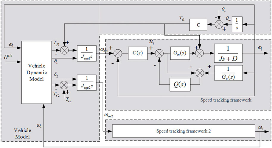
FIGURE 8. Control diagram of load simulation system under non-uniform speed and non-uniform load conditions.
In the control process of the entire vehicle load simulation, each side’s driving wheel corresponds to a set of load simulation systems (referred to as subsystems below), and all subsystems receive instructions from the same control system to simulate the loads of each wheel, thereby achieving the load simulation of the entire vehicle. Therefore, there is also a problem of multi-motor synchronization control in the control of the entire vehicle load simulation system. In the process of multi-motor synchronization control, the differences in hardware and mechanics between the various independent subsystems make it difficult for the control system to keep the controlled variables of each motor in a linear relationship, resulting in synchronization errors. To solve this problem, this section takes the track-type vehicle load simulation system as an example and uses the idea of cross-coupling compensation to compensate for the deviation between the two motors.
The basic principle of compensation correction is to detect the synchronization error ε of the speed
The resulting framework for the overall vehicle control under straight-line driving can be obtained as shown in Figure 9.
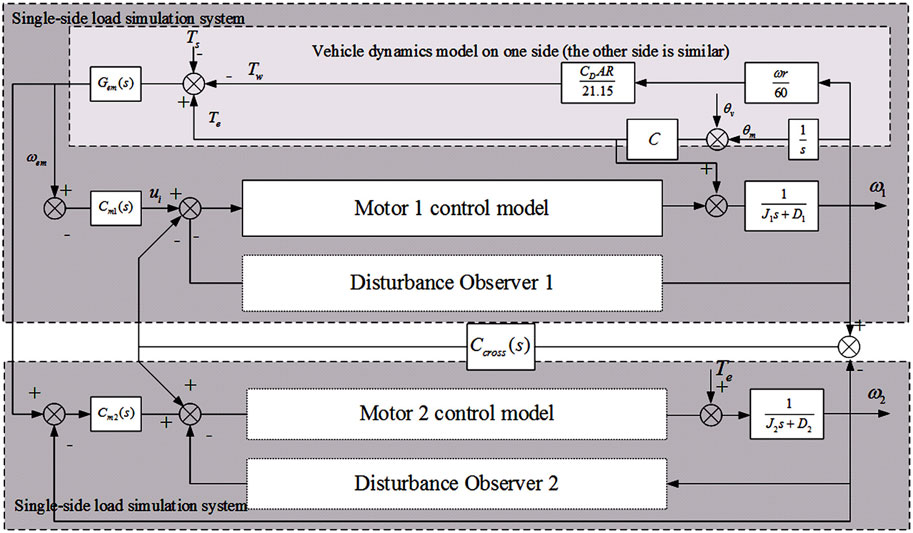
FIGURE 9. Cross-coupling compensation of the load simulation system under the condition of the same driving wheel speed.
A certain heavy-duty vehicle is subjected to dual-side load simulation. A virtual dashed line is used to indicate the enlarged position where a momentary torque disturbance of 500 Nm is applied to the left load simulation system. The simulation results are shown in Figure 10A. At t = 14s, the deviation of the left and right drive wheel speeds without considering cross-coupling compensation is about 0.3 rad/s. After taking cross-coupling compensation into consideration, both sides of the load simulation system generates a speed fluctuation of about 0.15 rad/s, but the relative speed deviation between the left and right sides has been reduced to 0.04 rad/s, and the synchronization of the system has been significantly improved.
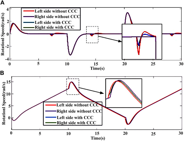
FIGURE 10. (A) Simulation curve of vehicle straight driving considering CCC (CCC is short for Cross-coupling compensation) under single-side pulse disturbance condition; (B) Simulation curve of vehicle straight driving considering CCC under single-side delay error condition.
A certain heavy-duty vehicle has been subjected to load simulation, and a system delay of 0.1s is given to the left-side load simulation system during the 10th second of the simulation. The simulation results are shown in Figure 10B. After the change of driving torque, due to the delay of the left-side system, there is a significant difference in the speed curves of the two sides, and the maximum value of the speed deviation at the same time is about 1.20 rad/s, which maintains a speed deviation of 0.38 rad/s after the speed fluctuation stabilizes. After considering the cross-coupling compensation, the maximum speed deviation drops to 0.24 rad/s, and quickly converges to 0, and the synchronization of the system is significantly improved.
Under the experimental conditions where the speeds on both sides are different, introducing Eq. 42 into Figure 8 yields the system control framework under different speed conditions, as shown in Figure 11. Unlike the cross-coupling compensation under straight-line driving conditions, since the speeds on both sides are different, it is necessary to first calculate the vehicle’s driving speed v using the speeds
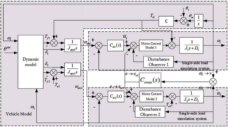
FIGURE 11. Cross-coupling compensation under different driving wheel speeds.
The same vehicle has been subjected to load simulation under steering conditions, with a uniform acceleration rotation of radius 50 m on a circular ramp with a slope of 10°. The speed response of both sides is shown in Figure 12.
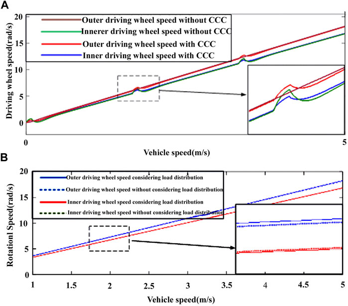
FIGURE 12. (A) Vehicle speed response under steering conditions; (B) Speed response of vehicle with consideration of CCC under steering condition.
As shown in Figure 12A, a disturbance with a pulse torque amplitude of 2000 Nm has been applied to the inner load simulation system, resulting in a speed fluctuation amplitude of 0.64 rad/s in the inner load simulation system due to the disturbance rejection effect of the disturbance observer. After taking the cross-coupling compensation into consideration, the outer speed fluctuates together with the inner speed, and the amplitude of the inner speed fluctuation decreases to 0.28 rad/s. The equivalent speed deviation between the two sides also decreases to 0.13 rad/s and quickly converges to 0. The synchronization of the system has been significantly improved.
As shown in Figure 12B, the speed response curve considering load distribution and slip ratio has a significant difference from the speed response curve without considering these factors. When the vehicle speed is 5 m/s, the inner speed response considering load distribution is 16.81 rad/s, and the speed response without considering load distribution is 16.98 rad/s, with a deviation of 1.01%. The outer speed response considering load distribution is 18.24 rad/s, and the speed response without considering load distribution is 17.95 rad/s, with a deviation of 1.58%.
The heavy-duty vehicle load simulation test bench mainly consists of a load simulation system and the test vehicle, and the test vehicle must be separated and enclosed in the environmental chamber to simulate various driving environments. Power compartments with load simulation motors and transmission mechanisms installed are located on both sides of the environmental chamber, as shown in Figures 13A, B. The transmission mechanism of the power compartment and the test vehicle inside the environmental chamber are connected through a through-wall shaft, as shown in Figures 13C, D. To prevent salt spray, sand, and other debris from entering the bearings, the walls at both ends of the through-wall shaft are mechanically sealed.
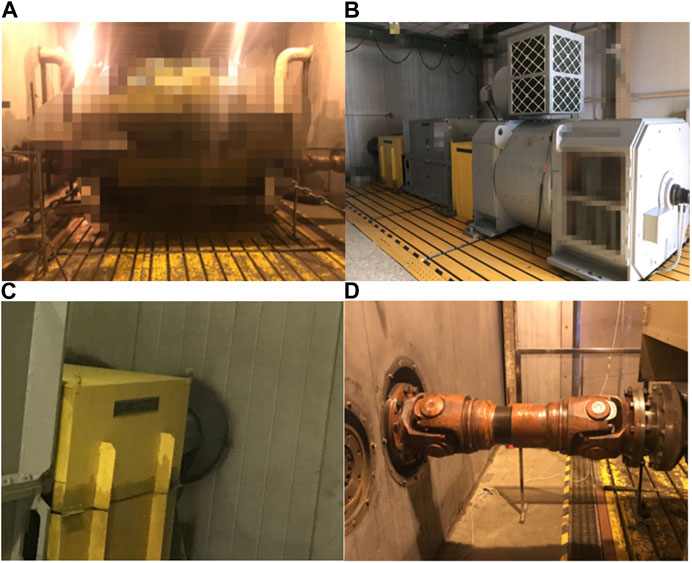
FIGURE 13. Mechanical structure of simulation device: (A) Environmental chamber; (B) Single-sided power compartment; (C) Through-wall shaft power compartment end; (D) Through-wall shaft environmental chamber end.
In this structure, by combining torque signals with the actual vehicle dynamics model, the target speed of the driving wheel and the speed of the high-power motor in the power compartment can be calculated, thereby achieving the goal of subjecting the driving wheel of the tested vehicle to the same load as the actual road driving (Fajri et al., 2012). The mechanical architecture of shaft coupling also ensures that the simulated loads between each subsystem are independent of each other, thus enabling the entire system to achieve composite working condition load simulation at the structural level.
During the testing process, the system controller needs to simultaneously control, calculate, and acquire data from both the test bench and the environmental chamber. As real-time calculations and motor control for both road load and inertial load are required during the testing process, the test system adopts a two-layer real-time control method for solving and controlling the load simulation system. During the testing process, the test management computer is responsible for managing, controlling, and displaying the testing project, and sends commands to the real-time control computer and PLC. The PLC is responsible for controlling the environmental simulator and collecting environmental signals to provide feedback to the test management computer. Two closed loops are formed between the real-time control computer and the electric motor, where the upper loop acquires the vehicle speed and steering signals and calculates/updates the real-time vehicle speed based on the whole vehicle kinematics model before sending it to the lower layer controller. The lower loop realizes the speed tracking control of each motor.
The control method of the single-side load simulation device that we use is speed tracking. During system operation, the board collects the steering angle signal
Load steering test is a test that studies the torque and speed during vehicle steering process. Through load steering test, the load condition of vehicle transmission equipment under steering conditions can be studied. For the test bench itself, the accuracy of simulating vehicle load steering can be verified through the test.
Figure 14 shows the test data of simulating a vehicle with a curb weight of 30t, turning left at a constant speed on a level ground with a radius of 50 m and a speed of 18 km/h. Due to the influence of the driver’s behavior on the driving speed of the vehicle, the measured stable driving speed of the vehicle is approximately 18.5 km/h. To determine the system response time under the preset spectrum, the experiment first verifies the system response time. According to Figure 14C, the average response time of the system is 25.40 m. The slowest response of the system torque occurs during several periods of significant torque fluctuations, during which the system speed fluctuates repeatedly. Due to system lag, the system is unable to respond in a timely manner, with a maximum response time of 68 m.
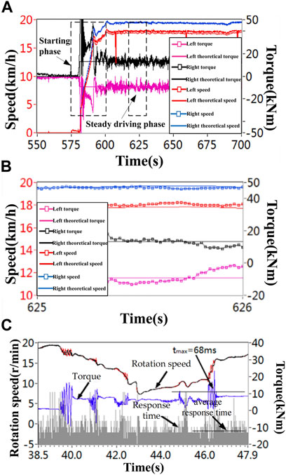
FIGURE 14. Load steering test: (A) Overall test data; (B) Amplified portion of data during stable driving phase; (C) System response time.
As shown in Figure 14A, during the startup phase, when the vehicle accelerates, the torque of the load motor fluctuates repeatedly to match the theoretical speed of the vehicle due to the response delay of the equipment. When the equipment enters the stable driving stage, as shown in Figure 14B, the theoretical values and the measured values of the left and right load simulation equipment are shown in Table 1.

TABLE 1. Experimental data for load steering test during stable driving phase.
Based on the data in Table 1, it can be seen that the error in both the speed and torque of the left-side load simulation equipment is higher than that of the right-side equipment, which is due to sampling errors in the torque and speed sensors on the left side. As there is a problem of asynchronous loading on the left and right sides during the steering simulation test, the internal load and speed on both sides may affect each other during the load simulation process. From Figure 14 and Table 1, it can be seen that the overall error of the equipment in the steering simulation process is less than 2.5%, indicating that the experimental platform designed in this paper can achieve accurate steering load simulation.
This paper studies the load simulation method for tracked vehicles under complex working conditions, based on the control strategy of single-axis load simulation system and the dynamic model of tracked vehicle during turning process. Firstly, the equivalent inertia allocated to the two wheels in different driving conditions are obtained through in-depth research on load allocation of vehicles under different driving conditions. To address the issue of synchronization errors in the motor during the complex working condition tests, the cross-coupling compensation method is used to reduce the synchronization errors. The experimental results show that the load simulation system considering equivalent inertia allocation and cross-coupling compensation has higher simulation accuracy and lower synchronization errors, and achieves accurate and engineering-meaningful load simulation for heavy-duty vehicles at the theoretical level.
The original contributions presented in the study are included in the article/Supplementary Material, further inquiries can be directed to the corresponding authors.
HL conceived the overall structure and framework of the article. GL conceived the outline of the manuscript. HL and GL wrote the manuscript and generated the figures. WC and JM helped to perform the manuscript with constructive discussions. In the process of revising the paper, ZC has made important contributions to the change of the overall framework and technical route of the paper. All authors contributed to the article and approved the submitted version.
Authors HL and JM were employed by the company Suzhou Sc-Solar Equipment Co., Ltd.
The remaining authors declare that the research was conducted in the absence of any commercial or financial relationships that could be construed as a potential conflict of interest.
All claims expressed in this article are solely those of the authors and do not necessarily represent those of their affiliated organizations, or those of the publisher, the editors and the reviewers. Any product that may be evaluated in this article, or claim that may be made by its manufacturer, is not guaranteed or endorsed by the publisher.
Bai, J., Wu, X., Gao, F., Li, H., and Yue, H. (2017). Modeling and simulation of multi-axle vehicle powertrain system[J]. J. Beijing Univ. Aeronautics Astronautics 43 (1), 136–143. doi:10.13700/j.bh.1001-5965.2016.0708
Bekker, M. G. (1960). Off-road locomotion: Research and development in terramechanics. Ann Arbor, Michigam: The Univ of Michigam press.
ChenZhouWang, Z. X. Z., Li, Y., and Hu, B. (2019). A novel emergency braking control strategy for dual-motor electric drive tracked vehicles based on regenerative braking. Appl. Sci. 9 (12), 2480. doi:10.3390/app9122480
Fajri, P., Ahmadi, R., and Ferdowsi, M. (2012). “Equivalent vehicle rotational inertia used for electric vehicle test bench dynamic studies[C],” in Proceedings of the 38th IEEE Industrial Electronics Society Annual Conference, 25-28 October 2012 (Montreal, QC, Canada: IEEE), 4115–4120.
Fajri, P., Ahmadi, R., and Ferdowsi, M. (2013). “Test bench for emulating electric-drive vehicle systems using equivalent vehicle rotational inertia[C],” in 2013 IEEE Power and Energy Conference at Illinois (PECI), Urbana, IL, USA, 22-23 February 2013 (IEEE), 83–87.
Fu, W. X., Sun, L., Yu, Y. F., Zhu, S. P., and Yan, J. (2009). Design and model-building of motor-driven load simulator with large torque outputs[J]. J. Syst. Simul. 21, 3596–3598.
Huh, K., Kim, J., and Hong, D. (2001). “Estimation of dynamic track tension utilizing a simplified tracked vehicle model [C],” in Proceedings of the American Control Conference, Arlington, VA, USA, 25-27 June 2001 (IEEE), 25–27.
Janarthanan, B., Padmanabhan, C., and Sujatha, C. (2011). Lateral dynamics of single unit skid-steered tracked vehicle. Int. J. Automot. Technol. 12 (6), 865–875. doi:10.1007/s12239-011-0099-4
Jiang, F., Dong, M., Fan, Y., and Wang, Q. (2022). Research on motor speed control method based on the prevention of vehicle rollover[J]. Energies 15, 3609. doi:10.3390/en15103609
Kim, J. H., Park, C. S., Kim, S. G., and Kim, J. H. (2003). Hydraulic system design and vehicle dynamic modeling for the analysis and development of tire roller[J]. Int. J. Control Autom. Syst. 1, 89–94.
Lv, H., Zhou, X., Yang, C., Wang, Z., and Fu, Y. (2019). Research on the modeling, control, and calibration technology of a tracked vehicle load simulation test bench. Appl. Sci. 9 (12), 2557. doi:10.3390/app9122557
Nam, Y. (2001). QFT force loop design for the aerodynamic load simulator. IEEE Trans. Aerosp. Electron. Syst. 37 (4), 1384–1392. doi:10.1109/7.976973
Ott, H., Degen, R., Leijon, M., and Ruschitzka, M. (2021). Model-based approach to investigate the influences of different load states to the vehicle dynamics of light electric vehicles[J]. Transp. Sci. Technol. 11 (02), 213–230. doi:10.4236/jtts.2021.112014
Takeda, M., Hosoyamada, Y., Motoi, N., and Kawamura, A. (2014). “Development of the experiment platform for electric vehicles by using motor test bench with the same environment as the actual vehicle,” in 2014 IEEE 13th International Workshop on Advanced Motion Control (AMC), Yokohama, Japan, 14-16 March 2014 (IEEE).
Wang, H., Song, Q., Wang, S., and Zeng, P. (2015). Dynamic modeling and control strategy optimization for a hybrid electric tracked vehicle. Math. Problems Eng. 2015, 1–12. doi:10.1155/2015/251906
Wang, H., and Sun, F. C. (2014). Dynamic modeling and simulation on a hybrid power system for dual-motor-drive electric tracked bulldozer. Appl. Mech. Mater. 494-495, 229–233. doi:10.4028/www.scientific.net/amm.494-495.229
Wang, Z., Lv, H., Zhou, X., Chen, Z., and Yang, Y. (2018). Design and modeling of a test bench for dual-motor electric drive tracked vehicles based on a dynamic load emulation method. Sensors 18, 1993. doi:10.3390/s18071993
Xingguo, M., Tao, Y., Xiaomei, Y., and Bin, Z. (2011). “Modeling and simulation of multibody dynamics for tracked vehicle based on RecurDyn [C],” in International Conference on Intelligent Networks & Intelligent Systems, Shenyang, China, 01-03 November 2010 (IEEE).
Yalla, S. K., Kareem, A., and Asce, M. (2007). Dynamic load simulator: Actuation strategies and applications. J. Eng. Mech. 133, 855–863. doi:10.1061/(asce)0733-9399(2007)133:8(855)
Yang, J., Zhou, X., Wei, Y., and Gong, R. (2013). Test bed modeling and control method for track vehicle. Trans. Chin. Soc. Agric. Mach. 44 (06), 8–13. doi:10.6041/j.issn.1000-1298.2013.06.002
Keywords: tracked vehicles, load simulation, complex working conditions, load distribution, testing technology
Citation: Lv G, Lv H, Chen Z, Chu W and Mao J (2023) Research on inertia transfer in load simulation of tracked vehicle under complex working conditions. Front. Mater. 10:1188411. doi: 10.3389/fmats.2023.1188411
Received: 17 March 2023; Accepted: 05 May 2023;
Published: 18 May 2023.
Edited by:
Guosong Wu, Hohai University, ChinaReviewed by:
Lin Mao, University of Shanghai for Science and Technology, ChinaCopyright © 2023 Lv, Lv, Chen, Chu and Mao. This is an open-access article distributed under the terms of the Creative Commons Attribution License (CC BY). The use, distribution or reproduction in other forums is permitted, provided the original author(s) and the copyright owner(s) are credited and that the original publication in this journal is cited, in accordance with accepted academic practice. No use, distribution or reproduction is permitted which does not comply with these terms.
*Correspondence: Haoliang Lv, bGhsODAxQHFxLmNvbQ==; Zhaomeng Chen, Y2hlcm56bUBzenB0LmVkdS5jbg==
Disclaimer: All claims expressed in this article are solely those of the authors and do not necessarily represent those of their affiliated organizations, or those of the publisher, the editors and the reviewers. Any product that may be evaluated in this article or claim that may be made by its manufacturer is not guaranteed or endorsed by the publisher.
Research integrity at Frontiers
Learn more about the work of our research integrity team to safeguard the quality of each article we publish.