 Joachim Osterberger
 Franz Maier
 Roland Markus Hinterhölzl
- Research Group for Lightweight Design and Composite Materials, University of Applied Sciences Upper Austria, Wels, AUT, Austria
In order to demonstrate the accuracy of macroscopic finite element draping simulations it is necessary to compare the results with experiments. In this work, a compact overview of evaluation methods for draping simulations based on experiments, in the recent literature, is provided. Then, a method using state of the art 3D laser scans (RS6, Hexagon) and robot supported fiber angle scans (FScan, Profactor) is described. The presented comparison of draping results with the tool geometry in 3D allows for an evaluation of wrinkles and bridging areas. For the evaluation of the edge contour, the commonly used method of projecting the edge contour on a 2D plane is extended to a comparison in 3D space. To determine fiber orientations and compare them with the predictions from simulations, a robot supported fiber angle sensor and a script-based mapping and comparison algorithm are used. The results are further analyzed statistically, to derive comparative figures to other results found in the literature. The location and dimensions of macroscopic manufacturing effects such as fiber bridging and wrinkles could be predicted accurately. The final component contour could be on average predicted within 5.2 mm. The fiber orientation could be predicted with a deviation of less than 2° for approx. 65% and within 6° for 95% of the part surface for UD laminas. Cross-ply laminas showed larger deviations, only 40% of the part surface was within 2° and 80% within 6°, compared to the experiment. Overall, the results for the presented methods show good agreement between multi-ply draping experiments and macroscopic simulations conducted with the Abaqus Fabric material model.
1 Introduction
Macroscopic finite element (FE) forming simulations for manufacturing composite components have become increasingly important in the transportation industries over the last two decades. Demonstrating the accuracy builds the foundation for a reliable application and use of FE based draping simulations. Two main methods to validate draping simulations are commonly described in the literature. The first is to model mechanical testing procedures (i.e., virtual testing) and compare the simulation result with the measured response from experiments. This can also be used as an inverse approach to identify material parameters used in phenomenological material models. The second method is to perform draping experiments on generic demonstrator geometries, typically with challenging features, such as curvatures, a double curvature, or tapered surfaces. Thus, the semifinished compositematerials are exposed to complex deformation mechanisms. Depending on the used raw material, effects such as wrinkle formation can be easily triggered. This validation method provides details about the accuracy of the simulation results at quite extreme deformation conditions. Comparison methods typically focus on fiber orientations, wrinkle formation and position, and the edge contour in the deformed configuration. Various generic geometries are reported, whereby a complete hemisphere (Mohammed et al., 2000; Boisse et al., 2011; Peng and Ding, 2011; Bardl et al., 2016; Chen et al., 2016; Machado et al., 2016; Schirmaier et al., 2016; Han and Chang, 2018; Nasri et al., 2019; Mei et al., 2021) or hemispheric sections, combined with elongated sections (Willems, 2008; Vanclooster et al., 2009; Schug et al., 2018; Viisainen et al., 2021) are most common. Other methods include rectangular box shapes (Huang et al., 2021), potentially combined with a sinusoidal surface path (Leutz, 2016; Margossian, 2017; Osterberger et al., 2022) or tetrahedron geometries (Thompson et al., 2020; Chen et al., 2021; Viisainen et al., 2021). Geometries with sharp corner sections can potentially trigger large local deformations and wrinkle formation, depending on the raw material in use. Once the simulation has passed the validation on a generic demonstrator basis, the next step is to evaluate with increasingly complex application examples, e.g., egg box shape (Han and Chang, 2021a) or various complex preform geometries, as shown in (Alshahrani and Hojjati, 2017; Chen et al., 2017; Dörr et al., 2017; Mallach et al., 2017; Joppich, 2019). The different tooling geometries come with advantages and disadvantages depending on the material, for example, the hemisphere is very suitable for woven fabrics, while it damages UD-materials and leads to a large amount of wrinkles, due to large shear deformations (Leutz, 2016). Consequently, a wide range of geometries are proposed in the literature, making it challenging to generalize and compare results between studies.
Many different experimental methods to quantify the geometrical accuracy and manufacturing effects are proposed in the literature. For example, simple side-by-side comparison of simulation results with photographs (Margossian, 2017; Thompson et al., 2020; Huang et al., 2021), plotted stress- or strain results (Harrison et al., 2013; Chen et al., 2016; Alshahrani and Hojjati, 2017; Chen et al., 2017; Osterberger and Franz Maier, 2020; Han and Chang, 2021a), digital image correlation (DIC) measurements (Chen et al., 2021; Bai et al., 2022), and a 3D scan supported analysis (Dörr, 2019; Joppich, 2019; Osterberger et al., 2022) are used to evaluate wrinkling. Similarly, various methods are proposed to evaluate the edge contour, typically projected onto a plane. Common methods include a comparison with photographs (with or without grid points) and a simple ruler (with no specific standardized method or technique) (Mohammed et al., 2000; Leutz, 2016; Margossian, 2017; Nasri et al., 2019; Thompson et al., 2020; Han and Chang, 2021a; Mei et al., 2021; Rashidi et al., 2021), grid point analysis with a coordinate measurement machine (CMM) (Chen et al., 2016), analysis with DIC (Chen et al., 2021; Bai et al., 2022), up to 3D scan supported analysis (Dörr et al., 2017; Dörr, 2019; Joppich, 2019; Osterberger et al., 2022).
The simulated fiber angle distribution is typically validated by local comparison. Methods include a manual angle measurement with a protractor (Mohammed et al., 2000), grid strain analysis with a CMM (Chen et al., 2016), orthogonal photographs for analysis at predefined points with ImageJ software (Harrison et al., 2013), the marker tracking method, or grid pattern tracking with DIC systems and suitable software (Vanclooster et al., 2009; Nasri et al., 2019; Rashidi et al., 2021; Bai et al., 2022), and fully robot supported fiber angle sensor scans, allowing precise tracking of fiber angles on complex geometries on the surface, as presented in (Leutz, 2016; Mallach et al., 2017; Margossian, 2017; Malhan et al., 2021), or by the use of the eddy current method (Bardl et al., 2016).
In this paper a set of methods to gauge the accuracy of the macroscopic FE simulation with Abaqus *Fabric (Osterberger et al., 2022) is presented, on a single ply basis and with different thin layups. Single diaphragm forming is used as the automated draping process for our simulations and experiments. The method utilizes 3D laser scans (with a Hexagon RS6 laser scanner) for detailed evaluation of wrinkling and bridging from draping experiments, based on a comparison with the tooling geometry. A further investigation on the advantages of comparing the edge contour in 3D, rather than in 2D, as commonly found in recent literature, was conducted. Fiber angle orientations are measured with the robot supported FScan method, presented in (Leutz, 2016) and (Margossian, 2017), across the entire surface of the specimen.
2 Materials and methods
2.1 Material
For the experiments a carbon UD-prepreg (HexPly® M79/34%/UD300/CHS) with a low temperature curing epoxy system and an approximate ply thickness of 0.35 mm is used for the experiments.
2.2 Experimental setup
All draping experiments are performed on a single diaphragm forming station with a generic double sine tool (∼245 mm × 245 mm × 90 mm) according to the concept presented in (Osterberger et al., 2022). The blank laminate is fixed with a flexible magnetic clamping system and a PTFE separation film, used to prevent sticking to the membrane (c.f. Figure 1). The experiments are conducted with prepreg sheets of 260 × 220 mm in size. In addition to single ply experiments, the performance of four different layups was investigated: (0-0-0), (0-0-90), (0–90–0), (0–90), with three samples per layup. For more details on the experimental procedure the reader is referred to (Osterberger et al., 2022).
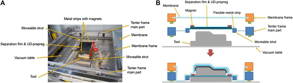
FIGURE 1. (A) Experimental setup at the diaphragms forming station prior to forming and (B) schematic cross-section view prior and during the forming step. Reprinted from (Osterberger et al., 2022).
2.3 Simulation setup
The FE simulation uses the Abaqus *Fabric material model and single ply modeling. Material characterization and modeling, as well as the FE model are shown in detail in (Osterberger et al., 2022). For the simulation of the four multi-layer laminates, the same basic setup was used, but modified in the following points: 1) Additional layers are modeled individually (as required for modeling the approximated bending behavior) as independent parts in Abaqus, positioned exactly above each other. Thus, the plies are in initial contact with each other, with friction in between the layers and the tooling and separation film as defined in (Osterberger et al., 2022). 2) To ensure contact while maintaining a common edge contour, allowing for shear and friction movement between plies, a tie connection along the outer edge contour of the plies, maintaining the initial inter-ply distance, was assigned. Rotational degrees of freedom (DOF) for the affected nodes were set free. 3) Gravity is only applied for a short time at the beginning of the simulation to establish the initial sag of the laminate, allowing an accurate prediction of the location of first contact with the tool. This allows for higher mass-scaling, i.e., virtually increasing the material density to reduce the critical time increment and thus, reduce the computational time, than initially proposed. Increasing the density by a factor 102 reduces the simulation time to 6–8 h (8-times faster), with the same hardware as presented in (Osterberger et al., 2022).
2.4 3D scanning
A portable RS6 laser scanner system, mounted on a Romer Absolute-Arm 8,520 (Hexagon) with a reported accuracy of 0.026 mm (2σ)was used for 3D scanning (Osterberger et al., 2022). Repeatability of the procedure was verified with a preliminary study. A slightly curved plate laminate (200 mm × 100 mm) made of PA6-UD tapes was scanned five times. Scans were then aligned and showed a maximum deviation of ± 0.05 mm for the surfaces at an edge length of 0.25 mm for the triangulated mesh.
The point cloud was obtained immediately after the forming step. The scanner allows for a scan rate of 300 Hz, however approximately 50% of measured points were filtered out to reduce calculation efforts, resulting in approximately 600.000 recorded points per second on a laser line with approximately 150 mm width. Scanning was completed within 1–2 min. After elimination of overlapping regions, about two million data points are used for comparison. The system enables 3D scans to be taken directly at the forming station without applying measurement markers or treatment with anti-reflexional coatings, which would compromise the surface for subsequent fiber angle scanning. The possible occurrence of deformations due to relaxation or creep effects in the prepreg material was minimized by measuring directly after the forming step. To improve positional alignment some concise areas of the tooling are included in each 3D scan. The software Control X (V2022.1, Geomagic) is used for data analysis.
2.5 Comparison of deformed shape
To determine wrinkling and bridging in the draped laminate the generated point cloud is triangulated with 0.05 mm edge length. This is five times smaller than in the preliminary study and therefore reduces the potential discretization error. Alignment of the experiment and the simulation is performed using the tool. The procedure is summarized in Figure 2.
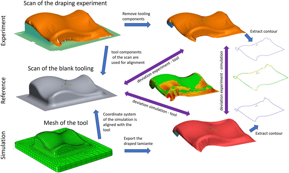
FIGURE 2. Summary of the alignment process and comparison methods used to evaluate the accuracy of the forming simulation.
Initially, the coordinate system of a 3D scan of the blank tooling and the discretized tooling used for the draping simulation are aligned via best-fit. The aligned tooling geometry then serves as reference for the alignment process with the draping experiment. Segments of the tooling that are not covered by the laminate are used for a local best-fit alignment. These regions are marked green in the scan of the draping experiment in the top left corner of Figure 2. This ensures that the laminate in the simulation and the experiment is aligned correctly. In a subsequent step the scans of the draping experiments are modified and protruding parts of the tooling are removed. The extracted, draped laminate is then used for a comparison with the reference tool surface for a detailed evaluation of wrinkles (position and size) and bridging areas (height and size) with the so-called 3D Compare tool in Control X. The deviations presented in this article are measured with the shortest distance method.
2.6 Comparison of edge contour
The correctly positioned scan of the draped geometry additionally serves as basis to extract the edge contour in 3D space. To compare it to the simulated edge contour, the draped geometry is exported from Abaqus (as triangulated mesh). Both geometries are already aligned via the tooling. The contour curves for the simulation and the experiment are extracted and deviations are measured with the shortest distance method, with the Curve Deviation tool in Control X. A smooth contour curve is generated from the discrete scan and simulation data via spline-interpolation and thus, can introduce an error. This effect is increased near corners, folds, or incomplete sections of the scan and for coarse (triangulated) meshes. A mesh size of 0.05 mm for the experiments resulted in an observed local error of up to ± 0.25 mm. The mesh size of the geometry exported from the simulation depends on the element size and was 5 mm in our case. Unfortunately, it is not possible to define more interpolation points or refine the edge contour otherwise in an automated way. Thus, slight deviations from the original simulated contours were unavoidable. Observed deviations stay within approximately ± 0.75 mm in sharp corners and are negligible in rather straight sections. This sums up to ± 1 mm possible systematic deviation due to discretization and interpolation.
2.7 Statistical analysis
To sum up the deviation of the laminate to the tooling geometry over all experiments, histograms are generated. Manufacturing effects such as fiber bridging and wrinkles cause a deviation while areas that are in contact to the tooling result in a deviation close to zero. To ensure comparable results, the same mesh densities, i.e., the density of data points distributed across the surface for each experiment, are used. Thus, after visualizing the wrinkles and extracting the edge contour, the mesh density for all experiments was reduced to get approximately 30.000 elements, corresponding to an element edge length of approximately 1.4 mm for the triangulated mesh. This is done for the geometry obtained from the experiment and the simulation. The deviation data is then exported to Matlab and histograms with an identical bin size are calculated, normalized, and averaged (in case of the experimental data).
2.8 Comparison of fiber angles
Fiber angles are measured using a photometric stereo sensor (FScan, Profactor), mounted on an industrial robot. The orientations are analyzed based on the directional dependency of the reflective properties of the material, with a reported root mean square error (RMSE) of up to 1.5° for prepreg materials (Zambal et al., 2015). For a detailed description of the comparison method, the reader is referred to (Keller et al., 2022). The procedure begins with placing the draped laminate, sitting on the tooling, on the measuring table and teaching the position of four reference points to the robot control system. This is done by moving a calibration tip to four dedicated locations on the tooling. These reference points allow for a coordinate transformation (via python script), where two reference points define the 0° or 90° direction. Subsequently, a robot path is planned with custom software from Profactor and the surface of the experiment is scanned automatically. The fiber angles across the surface are typically scanned in individual patches, that are stitched together and mapped onto the 3D geometry.
The orientation results, i.e., all measured points with their corresponding orientation vector, are exported (HDF5 file). A python script transforms the experimental data to the coordinate system of the simulation. A mapping algorithm (using a variation of the nearest neighbor method) is used to assign an average orientation vector from the FScan data to the corresponding mesh element of the draping simulation. For each element, a virtual sphere with a radius of 3 mm, centered in the mesh element (5 mm mesh size), is used to search for all FScan data points within this volume. An average value is calculated and assigned as orientation vector for the respective mesh element. Hence, for each mesh element the measured and simulated (extracted from Abaqus results via python script) local fiber orientations are available as a 3D vector. However, a direct comparison of two vectors in a 3D space is typically not intuitive. To simplify the comparison and quantify the difference to a single number, the orientation vectors are projected on a reference plane, which is derived from three of the measured reference points. This allows to determine the element-wise difference between simulation and experiment. The resolution of this fiber orientation/deviation map depends on the element-size of the FEM mesh. The used comparison method implies some limitations and drawbacks which are examined in (Keller et al., 2022) and summed up in the discussion below. Results are visualized within Abaqus by coloring the elements depending on the deviation using a python macro.
3 Results
3.1 Evaluation of deformed shape for single plies
For the evaluation on a single ply basis, a total of eight draping experiments were performed in the diaphragm station. Figure 3A illustrates deviations of the draping simulation and the tooling geometry, while Figures 3B–I shows deviations of the experiments to the tooling geometry. The 0° fiber direction is parallel to the global X-direction. A tolerance field of ± 0.5 mm is applied and set to a green color, indicating the material is in contact with the tool. The tolerance field is chosen slightly thicker than the ply thickness (0.35 mm), to compensate for systematic errors from FE meshing and alignment within the Control X software.
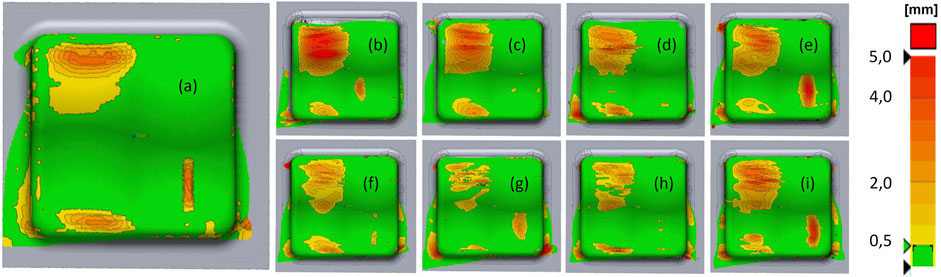
FIGURE 3. Comparison of the deformed shape from single ply (A) simulation and (B–I) experiments to the tool surface.
Aligning the meshed tool used for the FE analysis, with the 3D scan of the tooling, in order to align the coordinate systems of the simulation and the experiments, revealed a maximum local deviation (discretization error) of 0.4 mm in the lower left corner. The average deviation across the entire surface was 0 mm, with standard deviation (STD) of 0.1 mm.
Bridging and wrinkling are clearly visible in the results of the ply-to-tool comparison in Figures 3B–I and even very fine wrinkles (width of 1–2 mm) within a bridging area can be visualized.
The region showing bridging in the upper left corners is reasonably similar for all experiments, though the maximum height differs between 5 mm in Figure 3B and a minimum of 3 mm in Figure 3G, where the large bridging area is split up into several smaller ones. The area spanned by the bridging laminate is slightly underestimated in the simulation. Fine local wrinkles within this bridging area tend to be in the upper half of this area and correspond to the wrinkle indicated in the simulation.
Some variations between experiments are present, despite the effort made for providing reproducible experiments. Figures 3C, D, F, H, show no (or hardly any) wrinkle, i.e., red/yellow region in the lower right corner, while Figures 3B, E, G, I clearly do. Thus, this fold in the lower right corner appears only in 50% of the experiments, while it was found in the simulation as shown in Figure 3A. This location is a local maximum of the double sine geometry, and the simulation revealed that the material is locally compressed in this area. Thus, small instabilities during forming, slight misalignments of tooling or laminate, or local inhomogeneities (asymmetries) in the material can cause this fold to be pushed sideways, where it can dissipate.
Other regions with fiber bridging, one on the tooling surface along the lower edge of the double sine and another at the lower left corner, appear in the simulation and are also present in all experiments, with similar dimensions and height.
The simulation cannot cover fine wrinkles due to the coarse mesh size (5 mm). The histograms of the averaged 3D deviations from all experiments and the simulation, are shown in Figure 4.
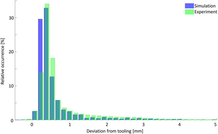
FIGURE 4. Summary of the 3D deviation distributions compared with the tool surface, on basis of eight single ply experiments vs. simulation in relative values.
The histograms are well aligned, indicating that the simulation and experiments follow the same trends. Large deviations from the tooling geometry (above 1 mm) are slightly underestimated by the simulation. Slight differences in the range of 0–0.5 mm are expected as this area is affected by discretization errors, occurring at the rounded corner sections of the tooling.
3.2 Evaluation of edge contour for single plies
For the analysis of the edge contour only five of the eight single ply experiments could be considered, due to an incomplete scan near the edge contour in the first three experiments (c.f. Figures 3B–D). Figure 5 shows a comparison of different views for the contour deviation of the part shown in Figure 3E. Figure 5A shows a projection onto a global X-Y plane, as it is commonly used in the literature. This method has some shortcomings when analysing complex 3D part geometries as out of plane deviation can visually disappear. This results in a discrepancy of arrow length and colour, where the latter is the reliable metric for the deviation. This becomes evident when comparing the regions 1 and 2 between views, as shown in Figures 5A–C. Thus, the contour deviation is presented in an isometric view. A tolerance field of ± 3 mm is chosen to consider for possible slight misalignment of the experiments and to consider systematic deviations coming from the chosen FE mesh discretization.
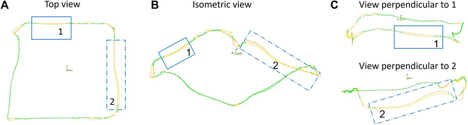
FIGURE 5. Comparison of the edge contour in (A) top (projected) view with (B) an isometric view; (C) Specific section could be further highlighted by adjusting the view, compromising the overall visibility.
The largest local deviations of up to 20 mm are present in Figure 6C. For the experiments in Figures 6A, B the edge contour matches the simulated contour very well, with maximum deviations of less than 8 mm. Larger deviations occurring on opposite sides, as visible in Figures 6C–E indicate a misalignment of the laminate for the experiments. The experimental procedure must be further improved to prevent this in future experiments. The contour deviations across all experiments are summarized in a histogram (Figure 7). An average deviation of 5.2 mm, a median of 4.5 mm, 25% quartile of 2.3 mm and 75% quartile of 7.2 mm are measured. Only occasional outliers above 14 mm are found.
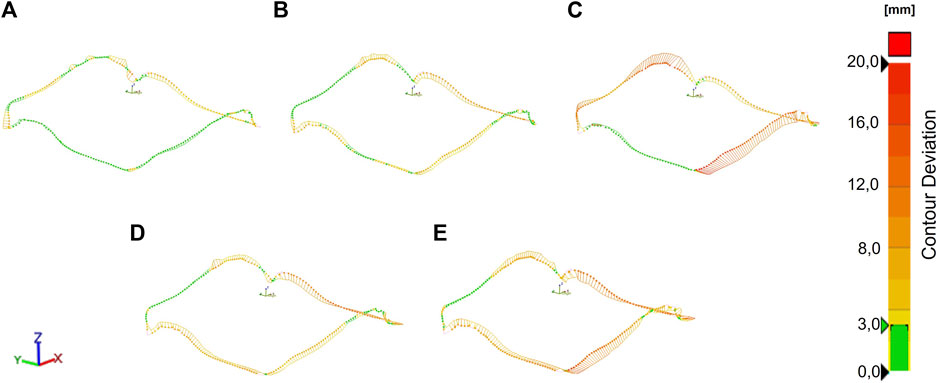
FIGURE 6. Comparison of the edge contour in 3D space from five single ply experiments (A–E) measured against the related simulation.
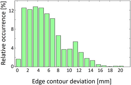
FIGURE 7. Distribution of edge contour deviations in 3D space, measured against the simulation, on basis of five single ply experiments.
3.3 Evaluation of deformed shape for multi-ply laminates
To evaluate the accuracy of the simulation for multi-ply laminas, three experiments are performed per layup. The results are presented in Figure 8. The 0° direction is aligned with the global X axis. The tolerance field for the green marked area varies between three-ply and two-ply layups due to the difference of lamina thickness. The range of the legend is kept at 5 mm, equivalent to the single ply experiments, while the tolerance field for three plies is defined with ± 1.2 mm and for two plies with ± 0.85 mm. Thus, a reasonably good comparability of 3D deviations at different laminate thicknesses is given.
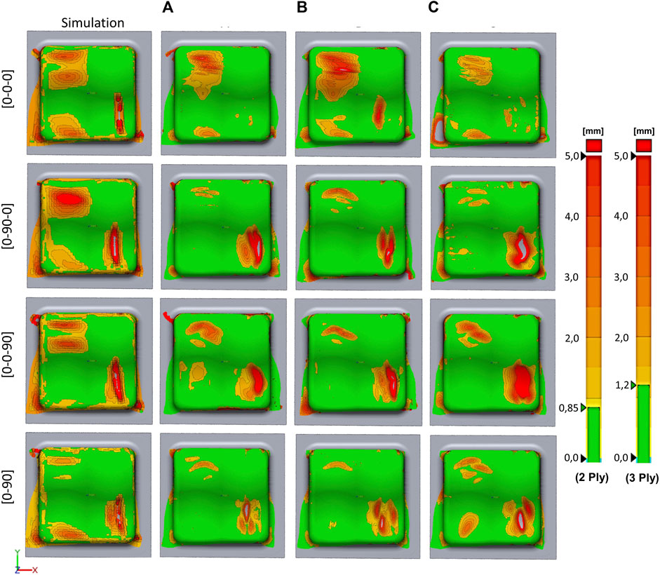
FIGURE 8. Comparison of the deformed shape from simulations (left gap) with four different layups (0-0-0), (0-0-90), (0-90-0), (0-90), three experiments per layup [gaps (A, B, C)], measured against the tool surface. The left legend applies to 3 ply laminas and the right one to 2 ply laminas.
In general, the simulations are capable of reproducing wrinkles and bridging areas on the top surface of the double sine tool geometry. Height and dimensions of wrinkles and bridging are captured with good accuracy for (0-0-0), (0-0-90) and (0-90) variants, however, in the (0-90-0) variant the bridging area in the upper left corner is overestimated. Deviations right at the laminate edges are generally overestimated and visible at the lower left corner of all simulations. This is caused by the tie connection enforced along the ply edges, preventing compression of the laminates in this area. However, this is a compromise allowing inter-ply movements, greatly improving the accuracy of the predicted contour.
A summary of the results shows that the FE simulation with Abaqus *Fabric presented in (Osterberger et al., 2022) is able to predict the position, size and shape of macro wrinkles and bridging areas of laminates quite well. The apparent differences between the experiments are likely caused by slight inhomogeneities in the raw material and differences in the material placements. The resolution of fine wrinkles is limited by the coarse mesh size (5 mm) but is considered sufficient for the presented case.
3.4 Evaluation of edge contour for multi-ply laminates
The results for the edge deviations, shown in Figure 9, correspond to the deformed shapes presented in Figure 8. The legend and the tolerance field are identical to the single ply experiments in Figure 6.
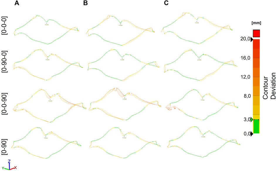
FIGURE 9. Comparison of the edge contour in 3D space from multi-ply experiments. Measured against the corresponding simulations. Four different layups (0-0-0), (0-0-90), (0-90-0), (0-90), three experiments per layup [gaps (A–C)], were realized.
In general, very good agreement of the edge contour was observed. Only for the (0-0-90) lamina larger deviations, especially in Z direction are visible in the lower left corner in column A and C. It appears that the specimen was detached from tooling after the draping process. It is unclear if this was due to some imperfections in the material that reduced tack, or if it was caused by residual stresses, surpassing the tack locally. This highlights the importance of scanning parts with a viscoelastic prepreg material type immediately after forming. The data from Figure 9 is summarized using boxplots in Figure 10. The median deviation depended on the lay-up and was smallest for the (0-0-0) and (0-90) laminates with 2.3 mm, followed by the (0-90-0) laminate, and largest for the (0-0-90) laminates with up to 6.2 mm. Local outliers, probably caused by detaching errors of specimens in corners are included in these reported values.
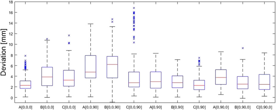
FIGURE 10. Boxplots of the edge contour analysis for all investigated specimens.
3.5 Evaluation of fiber orientations for multi-ply laminates
In Figure 11 the comparison method for the fiber angle measurement is shown exemplarily. The local fiber angle alignment predicted by the simulation, is shown in Figure 11A, the results from the scanning experiments are provided in Figure 11C, both are relative to the global X direction. A comparison of these two results is given in Figure 11B, where good agreement between the two data sets is shown and large deviations only occur near the edges and folds. Sections including large folds could not be scanned and are therefore grayed out. Preliminary tests of the undeformed raw prepreg material have been conducted to determine the material quality and results for the fiber angle deviation are presented in Table 1. While in 92% of the area of the UD prepreg sheet local misalignments where within 1.5°, localized deviations up to 3° must still be expected.
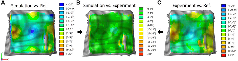
FIGURE 11. Fiber angle alignment: (A) simulation vs. reference direction (X direction), (B) simulation compared with experimental result, (C) experimental result vs. reference direction (X direction).
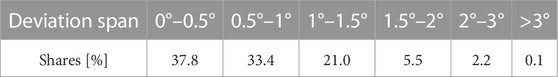
TABLE 1. Measured fiber angle distribution of the raw, undeformed material.
The comparisons of fiber angle orientations from the FE simulations with the individual corresponding experiments are shown in Figure 12. The shares per interval, visualized in Figure 12, are summarized in Figure 13.
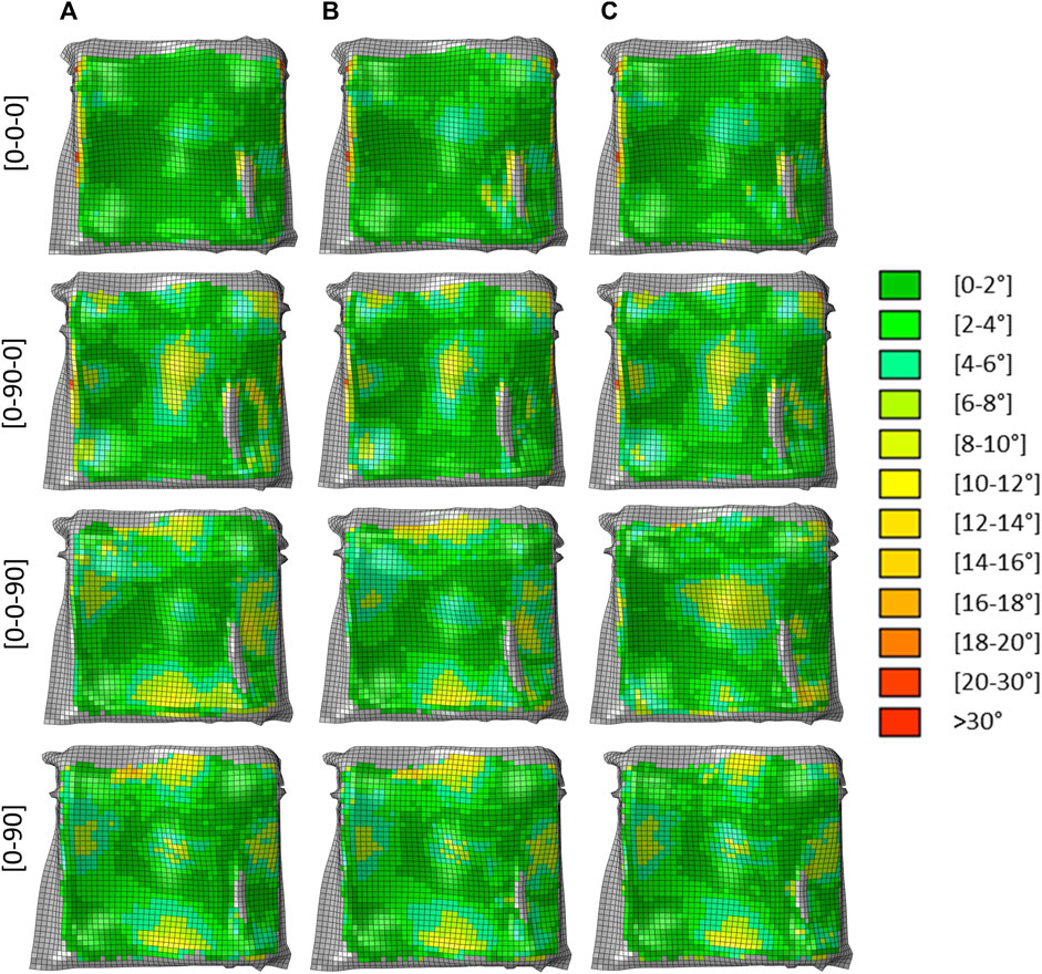
FIGURE 12. Comparison of fiber angle orientations derived from the FE simulations measured against four different experimental layups [(0-0-0), (0-0-90), (0-90-0), (0-90)] with three experiments per layup (A, B, C).
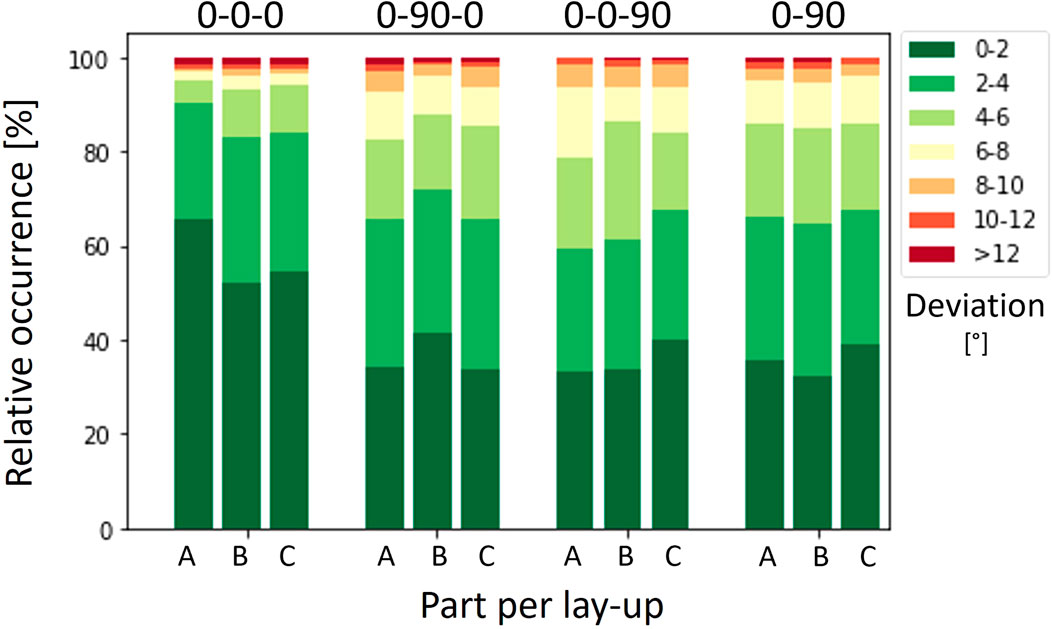
FIGURE 13. Shares for the fiber angle deviation between simulation and experiments for three parts (A, B, C) for four lay-ups, corresponding to Figure 12.
Best accuracy of fiber angles is reached for the (0-0-0) laminates, which is the only configuration where more than 80% of the surface was predicted within 0°–4°. For the other lay-ups only 60%–70% of the surface could be predicted within this range. This reduced accuracy could either originate from the fabric material or the contact definition and is subject of further investigations. Deviations between simulation and experiments above 12° are rare with a share of less than 2% across all experiments.
A systematic error when projecting the direction vector onto a plane, that depends on the angle of inclination of the corresponding element, was observed. However, both experiment and simulation are affected in a similar manner by this projection distortion, canceling out the systematic error. However, in strongly inclined regions (>30°) with large differences in simulated and measured fiber angles, the observed difference might be amplified.
4 Discussion
The evaluation of wrinkles and folds based on the 3D deviation from the tooling, as shown in Figures 3, 8, comes with the advantage, that the position and height of even fine wrinkles can be identified and visualized accurately. This is a clear advantage over comparison methods based on photographs or strain representations, e.g., in (Chen et al., 2016; Margossian, 2017; Han and Chang, 2018; Thompson et al., 2020; Huang et al., 2021). In (Chen et al., 2021) and (Bai et al., 2022) a detection method for wrinkles is shown based on data from a DIC system. Separate section cuts or a full surface comparison of the recorded Z amplitude are used, providing a similar degree of accuracy and capability to capture the entire surface, however, only big macro wrinkles were investigated in these cases. The overall quality, adhesion to the surface and integrity of the pattern can influence the applicability of DIC systems. It can become a limiting factor near locations that undergo large deformation, i.e., folds or wrinkles and subsequent curing steps might be affected by adding speckles to the surface. Utilizing the local curvature, as presented in (Dörr, 2019; Joppich, 2019; Kärger et al., 2020), can result in very exact tracking of the wrinkle formation in terms of occurrence and location, however cannot predict the height.
Thus, the main advantage of comparing 3D scans with the tool is the simultaneous visualization of wrinkles and bridging areas. In general, the method seems to be particularly applicable for the evaluation of draped parts with uncured, unstable semifinished products such as preforms made from prepreg or dry textiles. These parts would collapse when removed from the tooling before the final curing/infusion step to obtain the 3D scan. Recent generations of commercial laser scanners enable scanning of shiny surfaces without treatment of the surface, allowing for quick scans (less than a minute) between production steps. Exporting the deviation data (or raw location data) for each measurement, allows for further statistical analysis such as averaging of experimental results to improve comparability.
Analyzing the edge contour in the 3D space to evaluate draping experiments or simulations was not reported in the recent literature, to the authors’ best knowledge. By including information about the Z-direction, the possibility to detect deviations and their magnitude potentially increase. In-plane evaluation of the edge contour might cover up deviations of the part edge for complex 3D parts, as used, e.g., in (Dörr et al., 2017; Joppich, 2019; Han and Chang, 2021a). Thus, a direct comparison of our measured edge contour deviation between simulation and experiments with other literature is challenging due to varying raw material types.
A benchmark study comparing draping simulations for UD thermoplastic materials, conducted with PAM-Form, AniForm, LS-Dyna and Abaqus, reported contour deviations in the range of 8–10 mm (Dörr et al., 2017). Studies using an epoxy prepreg, but with a woven fabric, reported deviations up to 5 mm and 8 mm for a hemisphere and a pyramid, respectively (Chen et al., 2021) and up to 10 mm for a complex egg-box shape (Han and Chang, 2021a; Han and Chang, 2021b). Thus, the presented results (c.f. Figures 7, 10) are in a similar range, despite accounting for the total deviation in 3D and highlight the potential of the Fabric* material model for unidirectional, uncured prepreg materials. For the validation of forming simulations, it can be stated that using the 3D shaped edge contour allows to investigate the out-of-plane bending properties of the material. Projecting the deviation onto a plane, i.e., only observing the in-plane edge contours, e.g., (Peng and Ding, 2011; Nasri et al., 2019; Chen et al., 2021; Mei et al., 2021), validates mainly the in-plane shear properties.
Visualizing the fiber orientation on the entire 2D surface allows to capture and evaluate the full part geometry at once. The proposed method provides a visualization tool, using the same field of view as the FE simulations. This allows for quick full-field comparisons with a familiar user interface and avoids potential selection bias, that comes with methods that evaluate single predefined points or small patches on the surface as, e.g., in (Harrison et al., 2013; Mei et al., 2021; Rashidi et al., 2021; Bai et al., 2022). The photometric stereo metric method is limited to the top ply but the mapping algorithm could be used for other detection methods as well, e.g., the eddy current method (Bardl et al., 2016).
The method reduces the resolution from the original measurement by averaging values within a defined radius to match the element size of the FE mesh, but comparability is improved. This could be prevented by using finer FE-meshes, which would then increase the computational effort.
A limitation for this procedure is inherent to the measurement method and the geometrical properties of the FScan sensor. The photometric stereo procedure requires the sensor to be perpendicular and within a certain distance from the part surface (Zambal et al., 2015), thus the complexity of the part geometry can be limited by these constraints and the degrees of freedom in robot-movement. Thus, full-surface recording of complex 3D shapes as presented in (Mallach et al., 2017) is probably not possible. This could be prevented by using hand-guided fiber angle measurement systems such as the Apodius Vision System, presented in (Malhan et al., 2021). To prevent or reduce this limitation, multiple individual measurements could be obtained with individual scans and stitched together, assuming ideal alignment. The clear advantage lies in the automated nature of the procedure, which is ideal for repeated scans of identical parts.
Projecting our measured fiber angles onto a global projection plane introduces some uncertainty when the element surfaces are inclined more than 30° (0° would mean that the Element is parallel to the projection plane) (Keller et al., 2022). Areas with higher inclination angles are more prone to be affected by projection distortions. These systemic deviations are visible in Figure 12, where nearly all results show the highest deviations in areas with highest inclination angles. This could be resolved by defining not a single projection plane, but rather multiple regions reasonably parallel to the underneath surface. Alternatively, correction factors could be determined. However, within the scope of this project a global approach was pursued, and the method will be further improved in upcoming projects.
Comparing the fiber angle measurements in Figure 13 to the literature is again challenging. Typical evaluation methods either focus on a local assessment of absolute fiber orientation or report shear angles. While shear angles provide information about the local distortion of a fabric, they are neither suitable for unidirectional or NCF materials nor do they provide information about how well fibers are aligned with the intended orientation and the loading paths within the component. Reported local deviations in a range from 0°–3.3°, obtained with DIC (Bai et al., 2022), are well aligned with our findings for the (0-0-0) lamina, where up to 65% of the surface showed deviations below 2°. However, an evaluation on local points might be insufficient for a holistic assessment of predicted fiber orientations and might greatly underestimate the potential risk of material failure that can be caused by small, local weak spots. Global evaluations as presented in (Chen et al., 2016) for a biaxial non-crimp fabric (NCF) reported deviations up to 5°, which is similar to the values for the (0-0-0) layup. Layups including 90° plies generally show more locations with fiber orientations inaccurately predicted by our simulation. Fiber angle measurements for single ply draping experiments are not included in this study. A preliminary investigation was conducted with single ply experiments and generally less deviation between simulation and experiment, compared to multi-ply experiments, was found. In a representative experiment more than 70% of the surface was within 2° of the predicted fiber angles and approximately 95% of the surface within 4° and larger deviations were exclusively found at the edge or at folds (Keller et al., 2022).
This led to the conclusion that modelling of either the contact interaction including 90° or the in-plane shear properties of the material, using the *Fabric material model, are critical for the accuracy of the predicted fiber angles and targets for improvement.
The entire data acquisition was reasonably fast. Generating the 3D scans with the laser scanner took approximately 1–2 min and measuring the fiber angles with the FScan took approximately 3–5 min. Both durations depend on the part size and complexity. Increasing the part size increases the duration of manual laser scanning, while increasing complexity increases the duration of the automated fiber angles measurements. Data processing within Geomagic Control X requires manual data alignment and cleaning (local-best-fit with tool region, removing the tool data and contour smoothing) and took 10–15 min per part to obtain images, as shown in Figures 3, 8 for the surface deviationand Figures 6, 9 for the contour deviation. However, it is critical to align the coordinate system of the simulation with the experiment using the scan of the blank tooling. This ensures correct positioning and reduces the time for data processing. Visualizing the FScan Data (Figure 12) was fully automated via python scripts. Only the algorithm to map the measurement data onto the mesh took notable time (30 min at the time the presented results were generated but reduced to 3–5 min in the meantime due to software improvements).
The assessment of deviations from the intended shape and fiber orientation and their classification as tolerable effect or defect depends on their size, number and location within the component and the respective industry. Typically manufacturing effects that are highly disruptive to the load bearing capabilities and the fidelity of the shape, such as folds and fiber bridging are not acceptable. The formation of fiber wrinkles or fiber waviness on the other side, can be within the allowable strength reserve of the component (Thor et al., 2020). The maximum fiber angle deviations should typically be within 3°–5° of the direction specified in the development process for aviation and space industries, to guarantee the components strength and other anisotropic properties, e.g., thermal expansion. This range might be larger for automotive and nautical applications.
To correctly visualize and, more importantly, quantify these deviations requires a full-field assessment and comparison as proposed in this paper. In the presented case the method was used to gauge the applicability of the Abaqus Fabric* material model for draping simulations of thin laminas by comparing simulation results with experiments.
Regions where bridging and folds occur, as well as the final part contour were predicted accurately. The fiber angle was predicted within 6° for more than 95% of the surface of the investigated geometry for unidirectional, thin lay-ups. The accuracy drops to less than 80% predicted within 6° for lay-ups containing 0° and 90° plies, emphasizing the need to improve the contact properties in the simulation.
The proposed assessment method provides fast, quantifiable results and can be used to determine the quality during the development or prototyping phase and for a small batch size.
The calibrated material and process model then allows to adjust the tooling geometry and the manufacturing process virtually to reduce the risk of manufacturing defects.
Data availability statement
The raw data supporting the conclusion of this article will be made available by the authors, without undue reservation. We currently have no means to make this large amount of data publicly available.
Author contributions
JO and FM carried out the experimental work, the data processing and defined the evaluation methods. SK developed the method and all phyton scripts necessary for the fiber angle comparison. RH supervised the project. All authors contributed to the article and approved the submitted version.
Acknowledgments
We thank our funding source, the Austrian Research Promotion Agency (FFG), for supporting us in the project ProSim (866878).
Conflict of interest
The authors declare that the research was conducted in the absence of any commercial or financial relationships that could be construed as a potential conflict of interest.
Publisher’s note
All claims expressed in this article are solely those of the authors and do not necessarily represent those of their affiliated organizations, or those of the publisher, the editors and the reviewers. Any product that may be evaluated in this article, or claim that may be made by its manufacturer, is not guaranteed or endorsed by the publisher.
References
Alshahrani, H., and Hojjati, M. (2017). Experimental and numerical investigations on formability of out-of-autoclave thermoset prepreg using a double diaphragm process. Compos. Part A Appl. Sci. Manuf.101, 199–214. doi:10.1016/j.compositesa.2017.06.021
Bai, R., Colmars, J., Chen, B., Naouar, N., and Boisse, P. (2022). The fibrous shell approach for the simulation of composite draping with a relevant orientation of the normals. Compos. Struct.285, 115202. doi:10.1016/j.compstruct.2022.115202
Bardl, G., Nocke, A., Cherif, C., Pooch, M., Schulze, M., Heuer, H., et al. (2016). Automated detection of yarn orientation in 3D-draped carbon fiber fabrics and preforms from eddy current data. Compos. Part B Eng.96, 312–324. doi:10.1016/j.compositesb.2016.04.040
Boisse, P., Hamila, N., Vidal-Sallé, E., and Dumont, F. (2011). Simulation of wrinkling during textile composite reinforcement forming. Influence of tensile, in-plane shear and bending stiffnesses. Compos. Sci. Technol.71, 683–692. doi:10.1016/j.compscitech.2011.01.011
Chen, B., Colmars, J., Naouar, N., and Boisse, P. (2021). A hypoelastic stress resultant shell approach for simulations of textile composite reinforcement forming. Compos. Part A Appl. Sci. Manuf.149, 106558. doi:10.1016/j.compositesa.2021.106558
Chen, S., McGregor, O. P. L., Endruweit, A., Elsmore, M. T., De Focatiis, D. S. A., Harper, L. T., et al. (2017). Double diaphragm forming simulation for complex composite structures. Compos. Part A Appl. Sci. Manuf.95, 346–358. doi:10.1016/j.compositesa.2017.01.017
Chen, S., McGregor, O. P. L., Harper, L. T., Endruweit, A., and Warrior, N. A. (2016). Defect formation during preforming of a bi-axial non-crimp fabric with a pillar stitch pattern. Compos. Part A Appl. Sci. Manuf.91, 156–167. doi:10.1016/j.compositesa.2016.09.016
Dörr, D., Brymerski, W., Ropers, S., Leutz, D., Joppich, T., Kärger, L., et al. (2017). A benchmark study of finite element codes for forming simulation of thermoplastic UD-Tapes. Procedia CIRP66, 101–106. doi:10.1016/j.procir.2017.03.223
Dörr, D. (2019). Simulation of the thermoforming process of UD fiber-reinforced thermoplastic tape laminates. Karlsruhe: KIT Scientific Publishing.
Han, M. G., and Chang, S. H. (2018). Draping simulation of carbon/epoxy plain weave fabrics with non-orthogonal constitutive model and material behavior analysis of the cured structure. Compos. Part A Appl. Sci. Manuf.110, 172–182. doi:10.1016/j.compositesa.2018.04.022
Han, M. G., and Chang, S. H. (2021a). Draping simulations of carbon/epoxy fabric prepregs using a non-orthogonal constitutive model considering bending behavior. Compos. Part A Appl. Sci. Manuf.148, 106483. doi:10.1016/j.compositesa.2021.106483
Han, M. G., and Chang, S. H. (2021b). Simulation of the compressive behaviour of a composite egg-box core with fibre orientation-mapping technique and progressively degraded material properties. Compos. Part A Appl. Sci. Manuf.142, 106272. doi:10.1016/j.compositesa.2021.106272
Harrison, P., Gomes, R., and Curado-Correia, N. (2013). Press forming a 0/90 cross-ply advanced thermoplastic composite using the double-dome benchmark geometry. Compos. Part A Appl. Sci. Manuf.54, 56–69. doi:10.1016/j.compositesa.2013.06.014
Huang, J., Boisse, P., Hamila, N., Gnaba, I., Soulat, D., and Wang, P. (2021). Experimental and numerical analysis of textile composite draping on a square box. Influence of the weave pattern. Compos. Struct.267, 113844. doi:10.1016/j.compstruct.2021.113844
Joppich, T. D. (2019). Beitrag zum Umformverhalten von PA6/CF Gelegelaminaten im nicht-isothermen Stempelumformprozess. Karlsruhe: Karlsruher Institut für Technologie KIT.
Kärger, L., Galkin, S., Dörr, D., and Poppe, C. (2020). Capabilities of macroscopic forming simulation for large-scale forming processes of dry and impregnated textiles. Procedia Manuf.47, 140–147. doi:10.1016/j.promfg.2020.04.155
Keller, S., Maier, F., and Joachim Osterberger, R. M. (2022). “Hinterhölzl Comparing local fiber angles from draping experiments to simulations,” in Proceedings of the ECCM20, 20th European conference on composite materials (Lausanne, Switzerland: ECCM). doi:10.5075/epfl-298799_978-2-9701614-0-0
Leutz, D. M. (2016). Forming simulation of AFP material layups: Material characterization, simulation and validation. München: Technische Universität München TUM.
Machado, M., Fischlschweiger, M., and Major, Z. (2016). A rate-dependent non-orthogonal constitutive model for describing shear behaviour of woven reinforced thermoplastic composites. Compos. Part A Appl. Sci. Manuf.80, 194–203. doi:10.1016/j.compositesa.2015.10.028
Malhan, R. K., Shembekar, A. V., Kabir, A. M., Bhatt, P. M., Shah, B., Zanio, S., et al. (2021). Automated planning for robotic layup of composite prepreg. Robot. Comput. Integr. Manuf.67, 102020. doi:10.1016/j.rcim.2020.102020
Mallach, A., Härtel, F., Heieck, F., Fuhr, J. P., Middendorf, P., and Gude, M. (2017). Experimental comparison of a macroscopic draping simulation for dry non-crimp fabric preforming on a complex geometry by means of optical measurement. J. Compos. Mat.51, 2363–2375. doi:10.1177/0021998316670477
Margossian, A. (2017). Forming of tailored thermoplastic composite blanks: Material characterisation, simulation and validation. München: Technische Universität München TUM.
Mei, M., He, Y., Yang, X., and Wei, K. (2021). Analysis and experiment of deformation and draping characteristics in hemisphere preforming for plain woven fabrics. Int. J. Solids Struct.222–223, 111039. doi:10.1016/j.ijsolstr.2021.111039
Mohammed, U., Lekakou, C., and Bader, M. G. (2000). Experimental studies and analysis of the draping of woven fabrics. Compos. Part A Appl. Sci. Manuf.31, 1409–1420. doi:10.1016/S1359-835X(00)00080-4
Nasri, M., Garnier, C., Abbassi, F., Labanieh, A. R., Dalverny, O., and Zghal, A. (2019). Hybrid approach for woven fabric modelling based on discrete hypoelastic behaviour and experimental validation. Compos. Struct.209, 992–1004. doi:10.1016/j.compstruct.2018.10.081
Osterberger, J., and Franz Maier, R. H. (2020). “Process modelling of diaphragm forming with UD semi-finished prepregs,” in Proceedings of the SAMPE europe conference (Amsterdam, Netherlands: SAMPE), 8.
Osterberger, J., Maier, F., and Hinterhölzl, R. M. (2022). Application of the Abaqus *fabric model to approximate the draping behavior of UD prepregs based on suited mechanical characterization. Front. Mat.9, 865477. doi:10.3389/fmats.2022.865477
Peng, X., and Ding, F. (2011). Validation of a non-orthogonal constitutive model for woven composite fabrics via hemispherical stamping simulation. Compos. Part A Appl. Sci. Manuf.42, 400–407. doi:10.1016/j.compositesa.2010.12.014
Rashidi, A., Montazerian, H., and Milani, A. S. (2021). Slip-bias extension test: A characterization tool for understanding and modeling the effect of clamping conditions in forming of woven fabrics. Compos. Struct.260, 113529. doi:10.1016/j.compstruct.2020.113529
Schirmaier, F. J., Weidenmann, K. A., Kärger, L., and Henning, F. (2016). Characterisation of the draping behaviour of unidirectional non-crimp fabrics (UD-NCF). Compos. Part A Appl. Sci. Manuf.80, 28–38. doi:10.1016/j.compositesa.2015.10.004
Schug, A., Kapphan, G., Bardl, G., Hinterhölzl, R., and Drechsler, K. (2018). “Comparison of validation methods for forming simulations,” in Proceedings of the AIP conference proceedings (Palermo, Italy: AIP Publishing).
Thompson, A. J., Belnoue, J. P. H., and Hallett, S. R. (2020). Modelling defect formation in textiles during the double diaphragm forming process. Compos. Part B Eng.202, 108357. doi:10.1016/j.compositesb.2020.108357
Thor, M., Sause, M. G. R., and Hinterhölzl, R. M. (2020). Mechanisms of origin and classification of out-of-plane fiber waviness in composite materials—a review. J. Compos. Sci.4, 130. doi:10.3390/jcs4030130
Vanclooster, K., Lomov, S. V., and Verpoest, I. (2009). Experimental validation of forming simulations of fabric reinforced polymers using an unsymmetrical mould configuration. Compos. Part A Appl. Sci. Manuf.40, 530–539. doi:10.1016/j.compositesa.2009.02.005
Viisainen, J. V., Hosseini, A., and Sutcliffe, M. P. F. (2021). Experimental investigation, using 3D digital image correlation, into the effect of component geometry on the wrinkling behaviour and the wrinkling mechanisms of a biaxial NCF during preforming. Compos. Part A Appl. Sci. Manuf.142, 106248. doi:10.1016/j.compositesa.2020.106248
Willems, A. (2008). Forming simulation of textile reinforced composite shell structures. PhD Thesis. Leuven, Belgium: katholieke Universiteit Leuven.
Keywords: draping, laser scan, fiber angle scan, simulation, draping simulation, simulation validation
Citation: Osterberger J, Maier F, Keller S and Hinterhölzl RM (2023) Evaluation of draping simulations by means of 3D laser scans and robot supported fiber angle scans. Front. Mater. 10:1133788. doi: 10.3389/fmats.2023.1133788
Received: 29 December 2022; Accepted: 26 June 2023;
Published: 12 July 2023.
Edited by:
Clemens Dransfeld, Delft University of Technology, NetherlandsReviewed by:
Ewald Fauster, University of Leoben, AustriaMiro Duhovic, Leibniz-Institut für Verbundwerkstoffe, Germany
Copyright © 2023 Osterberger, Maier, Keller and Hinterhölzl. This is an open-access article distributed under the terms of the Creative Commons Attribution License (CC BY). The use, distribution or reproduction in other forums is permitted, provided the original author(s) and the copyright owner(s) are credited and that the original publication in this journal is cited, in accordance with accepted academic practice. No use, distribution or reproduction is permitted which does not comply with these terms.
*Correspondence: Franz Maier, ZnJhbnoubWFpZXJAZmgtd2Vscy5hdA==