Modeling systems from partial observations

Modeling systems from collected data faces two main difficulties: the first one concerns the choice of measurable variables that will define the learnt model features, which should be the ones concerned by the addressed physics, optimally neither more nor less than the essential ones. The second one is linked to accessibility to data since, generally, only limited parts of the system are accessible to perform measurements. This work revisits some aspects related to the observation, description, and modeling of systems that are only partially accessible and shows that a model can be defined when the loading in unresolved degrees of freedom remains unaltered in the different experiments.

1 Introduction

Simulation-based engineering (SBE) considers well-experienced physics-based models that are expected to describe the reality under scrutiny. These models must be calibrated from experiments in order to fine-tune the different parameters they involve. After that, they can be used to make predictions on the evolution of the considered system. The numerical solution of these models needs adequate numerical techniques to discretize the partial differential equations by which they are usually described, as well as powerful computing platforms to solve them efficiently.

Such a rationale was the main driving factor of last century engineering and faces two main limitations. The first handicap we must face is the fact that engineering is nowadays more concerned with performance than with the products themselves. Thus, engineering is expected to follow-up or monitor its designs all along their lives, resulting in the so-called Digital Twins, Tuegel et al. (2011); Chinesta et al. (2020); Ghanem et al. (2022); Kapteyn and Willcox (2020); Moya et al. (2022b); Argerich et al. (2020); Sancarlos et al. (2021b, a). However, they use craves for fast and accurate responses, and SBE often found difficulties to encompass real-time feedback. This limitation was alleviated by use of advanced model order reduction techniques Chinesta et al. (2011), Chinesta et al. (2013), Chinesta et al. (2014), Chinesta et al. (2015); Ibáñez et al. (2018); Borzacchiello et al. (2019); Sancarlos et al. (2021c). The second difficulty appears when the model solution exhibits a significant deviation with respect to the reality that it is expected to describe. The main reasons for the just mentioned deviations are incompleteness of models to recreate a complex reality and the intrinsic uncertainty and variability in our approximation to the physical reality.

Recent machine learning techniques enable alleviating the just referred limitations within the so-called fourth paradigm of sciences. On the one hand, accurate regressions can be constructed from the input/output data, which will later allow for collection of the output from the input in almost real-time, like model order reduction techniques (referred previously) performed on the solution of the complex mathematical models. The data manipulated by machine learning techniques can be experimental or synthetic (coming from high-fidelity simulations). On the other hand, when the considered data come from the real system, assumed free of noise, the learnt model will represent the reality in a very accurate manner, sometimes with higher accuracy than the existing physics-based models, Fasel et al. (2022).

In between the fully physics-based and the fully data-driven perspectives, an intermediate setting exists: the so-called hybrid paradigm, at the origin of the so-called Hybrid Twins Chinesta et al. (2020), that can be viewed as instances of physics-augmented learning or transfer learning, Weiss et al. (2016).

When considering machine learning techniques, the choice is very large. First, the adequate technique depends on the type of data to be manipulated. There are powerful tools to process images [e.g., convolutional neural networks, CNNs, Venkatesan and Li. (2017)], graphs [e.g., graph neural networks, GNNs, Bronstein et al. (2021) Hernandez et al. (2022)], time series [e.g., recurrent neural networks, rNNs, and long short-time memory, LSTM, Hochreiter and Schmidhuber (1997); Zhou et al. (2016)] .When data are very rich, many correlations may exist, and prior to proceeding with modeling, data-reduction seems a valuable route, with many manifold learning approaches available. Nonlinear dimensionality reduction can be efficiently performed in a nonlinear setting by using, for example, auto-encoders Goodfellow et al. (2016); Schmidhuber (2015); Hinton and Zemel (1993). Sparse autoencoders are of particular importance Ng (2011); Makhzani and Frey (2014).

When proceeding with data for modeling purposes, a recurrent issue concerns data accessibility. Sometimes, the considered system is not globally accessible, with only a small part of it being accessible to perform measurements.

The present study addresses a conceptual issue that will be discussed on an example simple enough to be fully understood, and at the same time complex enough to encompass all the modeling issues discussed in the present study.

The main question could be formulated as follows: if there is a part of a system inaccessible for observation in which a loading that we cannot either observe or measure applies, and that influences the measures performed in the observable part of the system, different questions arise:

• is there a model connecting the observable input(s) to its output(s), knowing that they are impacted by the hidden dynamics of the system? Is it unique?

• Under which conditions that model could exist? How to find it?

• How to formulate it correctly? Is it well-posed and consistent?

• How to learn it?

• What is the impact of these hidden dynamics on the learning process?

We referred previously to the use of rNN or LSTM, whose choice is guided by the knowledge gained from physics and mathematics, excellent allies of machine learning (ML). It is well-known that ML technologies such as rNN or LSTM allow us to manage, in transient problems, the hidden variables that, even if they are not observed, influence the evolution of the data in the observable regions Williams et al. (2022); Manohar et al. (2018).

This study aims at revisiting the construction of models in the domains exhibiting partial observability, in both the steady and transient cases, while following a double approach: the usual algebraic formulation and the one concerned by machine learning approaches.

2 On the existence of models relating observable features

In this section, we assume a large system, whose state is described by a number of state variables. We consider that the variables involved in the state description are well-defined. However, the model governing the state or its time evolution is assumed to be unknown, and the data describing the state are only observable and measurable on a part of the system, remaining unattainable in the rest of the system. Previous analysis on the field can be found in González et al. (2021) or Moya et al. (2022a).

For instance, in the case of the two-mass oscillator depicted in Figure 1, we assume that the state is perfectly defined by the position and momentum of each mass; however, only the state of the second mass is accessible (and thus, measurable). A natural question concerns the possibility of learning the model that governs the observable state (q₂, p₂) while ignoring the state of the first mass (q₁, p₁).

FIGURE 1

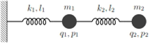
FIGURE 1. Oscillator composed of two masses, two linear springs of stiffness k₁ and k₂, reference lengths l₁ and l₂, and whose state is defined by the position and momentum of each mass (q₁, p₁, q₂, p₂).

In the following section, we address this question using a quite generic algebraic rationale in two situations: a model that does not depend on time and a transient problem. We will discuss the multiple-mass oscillators later. Henceforth, more generic settings are considered.

2.1 Time-independent problem

A generic linear time-independent model can be expressed from:

$\mathbf{K}\mathbf{U}=\mathbf{F},(1)$

which, considering the observable variables U_o and the internal ones U_i, can be rewritten as follows:

$\left(\begin{array}{cc}\hfill {\mathbf{K}}_{\mathbf{oo}}\hfill & \hfill {\mathbf{K}}_{\mathbf{oi}}\hfill \\ \hfill {\mathbf{K}}_{\mathbf{io}}\hfill & \hfill {\mathbf{K}}_{\mathbf{ii}}\hfill \end{array}\right)\left(\begin{array}{c}\hfill {\mathbf{U}}_{\mathbf{o}}\hfill \\ \hfill {\mathbf{U}}_{\mathbf{i}}\hfill \end{array}\right)=\left(\begin{array}{c}\hfill {\mathbf{F}}_{\mathbf{o}}\hfill \\ \hfill {\mathbf{F}}_{\mathbf{i}}\hfill \end{array}\right).(2)$

Developing the last equation, we find that

${\mathbf{K}}_{\mathbf{io}}{\mathbf{U}}_{\mathbf{o}}+{\mathbf{K}}_{\mathbf{ii}}{\mathbf{U}}_{\mathbf{i}}={\mathbf{F}}_{\mathbf{i}}\to {\mathbf{U}}_{\mathbf{i}}={\mathbf{K}}_{\mathbf{ii}}^{-1}{\mathbf{F}}_{\mathbf{i}}-{\mathbf{K}}_{\mathbf{ii}}^{-1}{\mathbf{K}}_{\mathbf{io}}{\mathbf{U}}_{\mathbf{o}}.(3)$

Also, introducing the resulting expression of U_i into the development of the first, we obtain (this is known as static condensation or Guyan reduction)

$\left({\mathbf{K}}_{\mathbf{oo}}-{\mathbf{K}}_{\mathbf{oi}}{\mathbf{K}}_{\mathbf{ii}}^{-1}{\mathbf{K}}_{\mathbf{io}}\right){\mathbf{U}}_{\mathbf{o}}={\mathbf{F}}_{\mathbf{o}}-{\mathbf{K}}_{\mathbf{oi}}{\mathbf{K}}_{\mathbf{ii}}^{-1}{\mathbf{F}}_{\mathbf{i}},(4)$

which can be rewritten as

${\tilde{\mathbf{K}}}_{\mathbf{oo}}{\mathbf{U}}_{\mathbf{o}}={\mathbf{F}}_{\mathbf{o}}-{\tilde{\mathbf{F}}}_{\mathbf{i}},(5)$

with

$\left\{\begin{array}{c}{\tilde{\mathbf{K}}}_{\mathbf{oo}}=\left({\mathbf{K}}_{\mathbf{oo}}-{\mathbf{K}}_{\mathbf{oi}}{\mathbf{K}}_{\mathbf{ii}}^{-1}{\mathbf{K}}_{\mathbf{io}}\right)\hfill \\ {\tilde{\mathbf{F}}}_{\mathbf{i}}={\mathbf{K}}_{\mathbf{oi}}{\mathbf{K}}_{\mathbf{ii}}^{-1}{\mathbf{F}}_{\mathbf{i}}\hfill \end{array}\right..(6)$

Remark 1:

• If F_i = 0, a direct relation exists between U_o and F_o.

• In the case of a 1D system in which only the borders of the interval are accessible (observable), U_o and F_o contain two components. If we apply ${{\mathbf{U}}_{\mathbf{o}}}^T=(\mathrm{1,0})$, the resulting F_o represents the first column of ${\tilde{\mathbf{K}}}_{\mathbf{oo}}$, and the solution F_o related to ${{\mathbf{U}}_{\mathbf{o}}}^T=(\mathrm{0,1})$ will represent the second column of ${\tilde{\mathbf{K}}}_{\mathbf{oo}}$.

• In the same one-dimensional system, when F_i ≠ 0, there are two effective internal variables, the components of ${\tilde{\mathbf{F}}}_{\mathbf{i}}$. Thus, all the richness of F_i endangers these two components, generating some sort of irreversibility: from F_i, we can obtain ${\tilde{\mathbf{F}}}_{\mathbf{i}}$, but from the last one, we cannot come back to the former. The condensation of the internal degrees of freedom into the observable one produces an entropy increase in the theory of information sense: there are many micro-states F_i associated with the macro-state ${\tilde{\mathbf{F}}}_{\mathbf{i}}$.

• Computing these two effective internal variables just referred needs extra-calculation. For example, if U_o = 0, then ${\mathbf{F}}_{\mathbf{o}}={\tilde{\mathbf{F}}}_{\mathbf{i}}$.

2.2 Time-dependent problem

A general linear second-order dynamical system can be expressed from

$\mathbf{M}\ddot{\mathrm{U}}+\mathbf{C}\dot{\mathrm{U}}+\mathbf{K}\mathbf{U}=\mathbf{F},(7)$

which, applying Fourier transform, becomes

$-{\omega }^2\mathbf{M}\mathbb{U}+i\omega \mathbf{C}\mathbb{U}+\mathbf{K}\mathbb{U}=\mathbb{F},(8)$

with $i\equiv \sqrt{-1}$ (without confusion with respect to other i subscript symbols used in the study, like the index i referring to the internal variables or the index i in vector components) and $\mathbb{U}$ and $\mathbb{F}$, the Fourier transforms of U and F , respectively. The previous equation can be rewritten as follows:

${\mathbf{K}}^{\ast }\mathbb{U}=\mathbb{F},(9)$

with K^∗ = −ω²M + iωC + K, that can be separated in the same way considered in the time-independent case, but now, for each possible frequency (ω) involved in the loading and operating in the complex domain, leading to

${\tilde{\mathbf{K}}}_{\mathbf{oo}}^{\ast }{\mathbb{U}}_{\mathbf{o}}={\mathbb{F}}_{\mathbf{o}}-{\tilde{\mathbb{F}}}_{\mathbf{i}},(10)$

which proves that all the discussion previously addressed in the time-independent case remains valid as soon as the Fourier transform applies.

Thus, one could expect that a model relating observable variables might exist as well (and could be learnt from collected data) in the time domain, under certain constraints, as the one referred in Remark 2 below, due to the dependence of ${\tilde{\mathbb{F}}}_i$ on the internal loading ${\mathbb{F}}_i$. This would imply the consideration of the history of the variables, which is naturally implicit in the Fourier transform. We will discuss this point later.

Remark 2:

The just-described rationale applies in the forced regime, i.e., far from the transient effects induced by the initial condition. In order to address transient regimes, the Laplace transform could be employed instead of the Fourier one. However, it is well-known that the Laplace inverse transform is less simple from the numerical point of view than Fourier’s. It is also important to note that the Fourier transform of the internal loading considered in the training stage should remain invariant to ensure the validity of the learnt model.

2.3 Neural network-based modeling

In many cases, artificial intelligence, and more concretely machine learning, aims at extracting the model that relates measured inputs to the corresponding outputs Brunton and Kutz (2019); Liu and Tegmark (2021). In general, the measured output depends on the whole internal state. For instance, in a structural dynamics problem where the loading (evolving in time) constitutes the problem’s input, the corresponding response is the displacement at each point and time, whereas the corresponding output data are the measured displacement in a certain observable point of the structure.

In physics-based structural mechanics, the internal response (displacement at any location and time instant) is obtained by discretization of the continuum mechanics model, consisting of the momentum balance and the constitutive equations; from this internal state, the output of interest is directly extracted at each time instant. Alternatively, machine learning looks for the direct relation between observables, the input action, and the measured response that, as just mentioned, can depend on the present and past values of a series of non-observed internal variables Lee and Carlberg (2020).

Recurrent neural networks (rNNs) and their long-short time memory counterparts (LSTM) address such situations by trying to model the time evolution of the internal state at the same time it constructs the model relating the observable input and output (action and response). For the sake of completeness, revisits both rNN and LSTM neural networks.

2.4 Addressing time-dependent problems in the time domain

Finally, to reinforce the main conclusions of Section 2.2, we are briefly discussing time-dependent problems modeling but directly operating in the time domain, instead of operating in the Fourier domain as was considered before. For simplicity, we contemplate the first-order dynamical system

$\mathbf{C}\dot{\mathbf{U}}+\mathbf{K}\mathbf{U}=\mathbf{F},(11)$

whose implicit time discretization reads

$\mathbf{C}{\mathbf{U}}^n+\mathrm{\Delta }t{\mathbf{K}\mathbf{U}}^n=\mathrm{\Delta }t{\mathbf{F}}^n+\mathbf{C}{\mathbf{U}}^{n-1},(12)$

with Δt being the considered time step. This equation can be rewritten in the more compact form

${\mathbf{K}}^{\ast }{\mathbf{U}}^n={\mathbf{F}}^{\ast ,n}+\mathbf{C}{\mathbf{U}}^{n-1},(13)$

with K^∗ = C + ΔtK and F^∗,n = ΔtFⁿ.

The sequencing of these equations can be written, inspired by the dynamic model decomposition, in the matrix form

${\mathbf{K}}^{\ast }\left[{\mathbf{U}}^n,\dots ,{\mathbf{U}}^1\right]=\left[{\mathbf{F}}^{\ast ,n},\dots ,{\mathbf{F}}^{\ast ,1}\right]+\mathbf{C}\left[{\mathbf{U}}^{n-1},\dots ,{\mathbf{U}}^0\right],(14)$

and by defining the extended vectors $\mathcal{U}$ and $\mathcal{F}$,

$\left\{\begin{array}{c}{\mathcal{U}}^T=\left[{\mathbf{U}}^{n^T},{\mathbf{U}}^{n-1^T},\dots ,{\mathbf{U}}^{0^T}\right]\hfill \\ {\mathcal{F}}^T=\left[{\mathbf{F}}^{n^T},{\mathbf{F}}^{n-1^T},\dots ,{\mathbf{F}}^{1^T}\right]\hfill \end{array}\right.,(15)$

and the extended matrix $\mathcal{K}$

$\mathcal{K}=\left(\begin{array}{ccccc}\hfill {\mathbf{K}}^{\ast }\hfill & \hfill -\mathbf{C}\hfill & \hfill \mathbf{0}\hfill & \hfill \dots \hfill & \hfill \dots \hfill \\ \hfill \mathbf{0}\hfill & \hfill {\mathbf{K}}^{\ast }\hfill & \hfill -\mathbf{C}\hfill & \hfill \mathbf{0}\hfill & \hfill \dots \hfill \\ \hfill \dots \hfill & \hfill \dots \hfill & \hfill \dots \hfill & \hfill \dots \hfill & \hfill \dots \hfill \end{array}\right),(16)$

The previous system reads

$\mathcal{K}\mathcal{U}=\mathcal{F},(17)$

where the solution $\mathcal{U}$ is, in general, computed from the $\mathcal{K}$ matrix pseudo-inverse.

This algebraic system can be addressed by using the same rationale that was applied before, but this time, the model will explicitly involve the time evolution of the input(s) and output(s), reinforcing the result already obtained when using the Fourier transform.

Another alternative formulation, more aligned with the use of machine learning techniques that will be presented afterward, consists of writing the explicit integration

$\mathbf{C}{\mathbf{U}}^n=\mathrm{\Delta }t{\mathbf{F}}^n-\mathrm{\Delta }t{\mathbf{K}\mathbf{U}}^{n-1}+\mathbf{C}{\mathbf{U}}^{n-1},(18)$

that can be reformulated as

${\mathbf{U}}^n=\mathbf{A}{\mathbf{F}}^n+\mathbf{B}{\mathbf{U}}^{n-1},(19)$

perfectly expressible within the rNN architecture illustrated in Figure 12. When the model concerns only a part of the state (the observable part), rNN and/or LSTM seem especially appealing to carry out the task.

3 Results

This section addresses, as indicated in the introduction, some numerical examples, simple enough to be perfectly understood, but complex enough to underline all the issues and methodological aspects just discussed.

One could think that working with a three-mass dynamical system while observing only the state of one of them is too simple. It is in fact very simple to visualize, and this was the primary objective: being easy to reproduce because such a model is quite simple to understand and replicate and check all the discussions that we are discussing in the present section.

However, this simplicity is only apparent. Forces are being applied to the internal masses, unknown and unobserved by the modeler, who, furthermore, totally ignores how many hidden masses are involved in the system. We consider three in the present example, but they could come in any number, from one to thousands.

When introducing all the system’s degrees of freedom—in our case, the state of the three masses—in a model, the last one becomes larger but finally simpler to interpret and to learn since all the needed data for properly describing the system are there, fully available. On the contrary, when considering only the data associated to one mass, while ignoring all the data related to all the other masses, the model seems simpler from its size, but very intricate nonetheless.

For this reason, and this was our motivation, the simplicity is only apparent and allows for a more fruitful discussion on the issues and the conceptual questions previously addressed.

For completeness, the different programs elaborated and used in the numerical examples addressed in the present section, in particular the rNN and LSTM neural network architectures (with their associated hyper-parameters), are available at https://github.com/cghnatios/LSTM-rNN-for-Modeling-systems-from-partial-observations-.git.

3.1 Learning in the Fourier space

We consider the linear N-mass dynamical system, including inertia, elastic, and damping behaviors, illustrated in Figure 2.

FIGURE 2

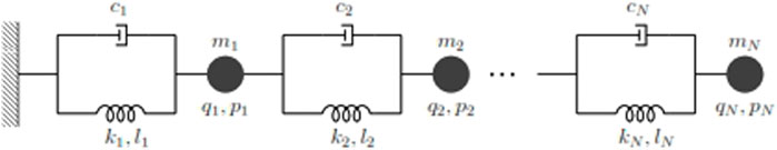
FIGURE 2. N-mass dynamical system.

The state of each mass is represented by z_i = (q_i, p_i), with q_i and p_i being the i-th mass position and momentum, respectively. We define the system state from the extended vector ${\mathbf{Z}}^T=({\mathbf{z}}_1^T,\dots ,{\mathbf{z}}_N^T)$.

The usual model, coming from Newton’s equation, can be expressed by

$\dot{\mathbf{Z}}=\mathbf{T}\mathbf{Z}+\mathbf{J}+\mathbf{F},(20)$

where matrix T includes the system properties, masses, spring stiffness, and viscosity of the dampers. On the other hand, J is a constant vector (in the linear case addressed below) and F contains the external forces applied to the different masses, appearing at odd positions in vector F (an explicit form of that matrix, and those vectors will be given later).

In the forced regime, the Fourier transformation becomes a valuable route. The dynamical model in the Fourier domain reads:

$\left(-\mathbf{T}+i\omega \mathbf{I}\right)\mathbb{Z}=\mathbb{J}+\mathbb{F}.(21)$

By defining the effective loading $\mathbb{S}=\mathbb{J}+\mathbb{F}$ and $\tilde{\mathbf{T}}=-\mathbf{T}+i\omega \mathbf{I}$, we can write the matrix form that separates the degrees of freedom related to the measurable position (noted by q) and the derived momentum (p):

$\left(\begin{array}{cc}\hfill {\tilde{\mathbf{T}}}_{qq}\left(\omega \right)\hfill & \hfill {\mathbf{T}}_{qp}\hfill \\ \hfill {\mathbf{T}}_{pq}\hfill & \hfill {\tilde{\mathbf{T}}}_{pp}\left(\omega \right)\hfill \end{array}\right)\left(\begin{array}{c}\hfill {\mathbb{Z}}_q\left(\omega \right)\hfill \\ \hfill {\mathbb{Z}}_p\left(\omega \right)\hfill \end{array}\right)=\left(\begin{array}{c}\hfill {\mathbb{S}}_q\left(\omega \right)\hfill \\ \hfill {\mathbb{S}}_p\left(\omega \right)\hfill \end{array}\right)=\left(\begin{array}{c}\hfill \mathbf{0}\hfill \\ \hfill {\mathbb{S}}_p\left(\omega \right)\hfill \end{array}\right).(22)$

Being ${\mathbb{S}}_q\left(\omega \right)=\mathbf{\text{0}}$, ${\mathbb{Z}}_p\left(\omega \right)$ can be expressed in terms of ${\mathbb{Z}}_q\left(\omega \right)$:

${\tilde{\mathbf{T}}}_{qq}\left(\omega \right){\mathbb{Z}}_q\left(\omega \right)+{\mathbf{T}}_{qp}{\mathbb{Z}}_p\left(\omega \right)=\mathbf{0}\to {\mathbb{Z}}_p\left(\omega \right)=-{\mathbf{T}}_{qp}^{-1}{\tilde{\mathbf{T}}}_{qq}\left(\omega \right){\mathbb{Z}}_q\left(\omega \right),(23)$

that, introduced into the second equation, leads to

$\left({\mathbf{T}}_{pq}-{\tilde{\mathbf{T}}}_{pp}\left(\omega \right){\mathbf{T}}_{qp}^{-1}{\tilde{\mathbf{T}}}_{qq}\left(\omega \right)\right){\mathbb{Z}}_q\left(\omega \right)={\mathbb{S}}_p\left(\omega \right),(24)$

which can be reshaped into a more compact form:

$\mathbf{A}\left(\omega \right)\mathbb{Q}\left(\omega \right)=\mathbb{R}\left(\omega \right),(25)$

with $\mathbf{A}\left(\omega \right)={\mathbf{T}}_{pq}-{\tilde{\mathbf{T}}}_{pp}\left(\omega \right){\mathbf{T}}_{qp}^{-1}{\tilde{\mathbf{T}}}_{qq}\left(\omega \right)$, $\mathbb{Q}\left(\omega \right)\equiv {\mathbb{Z}}_q\left(\omega \right)$, and $\mathbb{R}\left(\omega \right)\equiv {\mathbb{S}}_p\left(\omega \right)$.

This way, we have removed the momentum from the state variables since it derives directly from the measurable position.

Now, the partition between the internal and the observable degrees of freedom can be enforced:

$\left(\begin{array}{cc}\hfill {\mathbf{A}}_{\mathbf{oo}}\left(\omega \right)\hfill & \hfill {\mathbf{A}}_{\mathbf{oi}}\left(\omega \right)\hfill \\ \hfill {\mathbf{A}}_{\mathbf{io}}\left(\omega \right)\hfill & \hfill {\mathbf{A}}_{\mathbf{ii}}\left(\omega \right)\hfill \end{array}\right)\left(\begin{array}{c}\hfill {\mathbb{Q}}_{\mathbf{o}}\left(\omega \right)\hfill \\ \hfill {\mathbb{Q}}_{\mathbf{i}}\left(\omega \right)\hfill \end{array}\right)=\left(\begin{array}{c}\hfill {\mathbb{R}}_{\mathbf{o}}\left(\omega \right)\hfill \\ \hfill {\mathbb{R}}_{\mathbf{i}}\left(\omega \right)\hfill \end{array}\right)(26)$

such that following the aforementioned rationale leads to

${\tilde{\mathbf{A}}}_{\mathbf{oo}}\left(\omega \right){\mathbb{Q}}_{\mathbf{o}}\left(\omega \right)={\mathbb{R}}_{\mathbf{o}}\left(\omega \right)-{\tilde{\mathbb{R}}}_{\mathbf{i}}\left(\omega \right),(27)$

with ${\tilde{\mathbb{R}}}_{\mathbf{i}}\left(\omega \right)={\mathbf{A}}_{\mathbf{oi}}\left(\omega \right){\mathbf{A}}_{\mathbf{ii}}^{-1}\left(\omega \right){\mathbb{R}}_{\mathbf{i}}\left(\omega \right)$ and ${\tilde{\mathbf{A}}}_{\mathbf{oo}}\left(\omega \right)={\mathbf{A}}_{\mathbf{oo}}\left(\omega \right)-{\mathbf{A}}_{\mathbf{oi}}\left(\omega \right){\mathbf{A}}_{\mathbf{ii}}^{-1}\left(\omega \right){\mathbf{A}}_{\mathbf{io}}\left(\omega \right)$, where the same remarks that were previously discussed apply.

As a particular example, we consider a system composed of three identical masses (m₁ = m₂ = m₃ = m), springs (k₁ = k₂ = k₃ = k), and dampers (c₁ = c₂ = c₃ = c), with the springs having a reference length also identical (l₁ = l₂ = l₃ = l). Forces can be applied on both the internal masses (the first two) and on the observable one, the third. The following values are considered: m = 0.5 Kg, c = 0.8 N/m, k = 1 N/m, and l = 1 m.

The dynamical model reads

$\begin{array}{ll}\hfill \left(\begin{array}{c}\hfill {\dot{q}}_1\hfill \\ \hfill {\dot{p}}_1\hfill \\ \hfill {\dot{q}}_2\hfill \\ \hfill {\dot{p}}_2\hfill \\ \hfill {\dot{q}}_3\hfill \\ \hfill {\dot{p}}_3\hfill \end{array}\right)& =\left(\begin{array}{cccccc}\hfill 0\hfill & \hfill 1/m\hfill & \hfill 0\hfill & \hfill 0\hfill & \hfill 0\hfill & \hfill 0\hfill \\ \hfill -2k\hfill & \hfill -2c/m\hfill & \hfill k\hfill & \hfill c/m\hfill & \hfill 0\hfill & \hfill 0\hfill \\ \hfill 0\hfill & \hfill 0\hfill & \hfill 0\hfill & \hfill 1/m\hfill & \hfill 0\hfill & \hfill 0\hfill \\ \hfill k\hfill & \hfill c/m\hfill & \hfill -2k\hfill & \hfill -2c/m\hfill & \hfill k\hfill & \hfill c/m\hfill \\ \hfill 0\hfill & \hfill 0\hfill & \hfill 0\hfill & \hfill 0\hfill & \hfill 0\hfill & \hfill \frac{1}{m}\hfill \\ \hfill 0\hfill & \hfill 0\hfill & \hfill k\hfill & \hfill c/m\hfill & \hfill -k\hfill & \hfill -c/m\hfill \end{array}\right)\hfill \\ \hfill & \times \left(\begin{array}{c}\hfill q_1\hfill \\ \hfill p_1\hfill \\ \hfill q_2\hfill \\ \hfill p_2\hfill \\ \hfill q_3\hfill \\ \hfill p_3\hfill \end{array}\right)+\left(\begin{array}{c}\hfill 0\hfill \\ \hfill k_1{l}_1-k_2{l}_2\hfill \\ \hfill 0\hfill \\ \hfill k_2{l}_2-k_3{l}_3\hfill \\ \hfill 0\hfill \\ \hfill k_3{l}_3\hfill \end{array}\right)+\left(\begin{array}{c}\hfill 0\hfill \\ \hfill F_1\left(t\right)\hfill \\ \hfill 0\hfill \\ \hfill F_2\left(t\right)\hfill \\ \hfill 0\hfill \\ \hfill F_3\left(t\right)\hfill \end{array}\right),\hfill \end{array}(28)$

which, in the linear case and taking into account that k₁ = k₂ = k₃ = k and l₁ = l₂ = l₃ = l, after applying Fourier transform, leads to

$\begin{array}{ll}\hfill & \left(\begin{array}{cccccc}\hfill i\omega \hfill & \hfill -1/m\hfill & \hfill 0\hfill & \hfill 0\hfill & \hfill 0\hfill & \hfill 0\hfill \\ \hfill 2k\hfill & \hfill i\omega +2c/m\hfill & \hfill -k\hfill & \hfill -c/m\hfill & \hfill 0\hfill & \hfill 0\hfill \\ \hfill 0\hfill & \hfill 0\hfill & \hfill i\omega \hfill & \hfill -1/m\hfill & \hfill 0\hfill & \hfill 0\hfill \\ \hfill -k\hfill & \hfill -c/m\hfill & \hfill 2k\hfill & \hfill i\omega +2c/m\hfill & \hfill -k\hfill & \hfill -c/m\hfill \\ \hfill 0\hfill & \hfill 0\hfill & \hfill 0\hfill & \hfill 0\hfill & \hfill i\omega \hfill & \hfill -1/m\hfill \\ \hfill 0\hfill & \hfill 0\hfill & \hfill -k\hfill & \hfill -c/m\hfill & \hfill k\hfill & \hfill i\omega +c/m\hfill \end{array}\right)\hfill \\ \hfill & \times \left(\begin{array}{c}\hfill {\widehat{q}}_1\hfill \\ \hfill {\widehat{p}}_1\hfill \\ \hfill {\widehat{q}}_2\hfill \\ \hfill {\widehat{p}}_2\hfill \\ \hfill {\widehat{q}}_3\hfill \\ \hfill {\widehat{p}}_3\hfill \end{array}\right)=\left(\begin{array}{c}\hfill 0\hfill \\ \hfill 0\hfill \\ \hfill 0\hfill \\ \hfill 0\hfill \\ \hfill 0\hfill \\ \hfill kl\hfill \end{array}\right)\delta \left(\omega \right)+\left(\begin{array}{c}\hfill 0\hfill \\ \hfill {\widehat{F}}_1\hfill \\ \hfill 0\hfill \\ \hfill {\widehat{F}}_2\hfill \\ \hfill 0\hfill \\ \hfill {\widehat{F}}_3\hfill \end{array}\right),\hfill \end{array}(29)$

where the hat operator, $\widehat{•}$, refers to the Fourier transform of the mass positions, momentum, and applied forces.

It is important to note that, in the nonlinear case described later on, since the spring stiffnesses depend on the spring elongation and the latter will obviously be different for each node—unlike here in the linear case— the first vector of the right hand member will contain three non-vanishing spring contributions: k₁l₁ − k₂l₂, k₂l₂ − k₃l₃, and k₃l₃.

By reordering the previous system, the position and momentum degrees of freedom can be grouped:

and then, the momentum degrees of freedom ${\widehat{p}}_i$ condensed into the ones related to the mass positions ${\widehat{q}}_i$, as previously discussed:

$\left({\mathbf{T}}_{pq}-{\tilde{\mathbf{T}}}_{pp}\left(\omega \right){\mathbf{T}}_{qp}^{-1}{\tilde{\mathbf{T}}}_{qq}\left(\omega \right)\right){\mathbb{Z}}_q\left(\omega \right)={\mathbb{S}}_p\left(\omega \right).(31)$

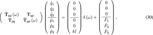
that, after separating the internal and observable degrees of freedom, reads

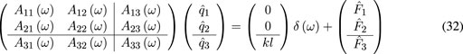
which allows making the model involving the observable degree of freedom, ${\widehat{q}}_3$, explicit:

$\begin{array}{ll}\hfill & \left\{A_{33}\left(\omega \right)-\left(\begin{array}{cc}\hfill A_{31}\left(\omega \right)\hfill & \hfill A_{32}\left(\omega \right)\hfill \end{array}\right)\right.\hfill \\ \hfill & \times \left.{\left(\begin{array}{cc}\hfill A_{11}\left(\omega \right)\hfill & \hfill A_{12}\left(\omega \right)\hfill \\ \hfill A_{21}\left(\omega \right)\hfill & \hfill A_{22}\left(\omega \right)\hfill \end{array}\right)}^{-1}\left(\begin{array}{c}\hfill A_{13}\left(\omega \right)\hfill \\ \hfill A_{23}\left(\omega \right)\hfill \end{array}\right)\right\}{\widehat{q}}_3\left(\omega \right)\hfill \\ \hfill & =kl\delta \left(\omega \right)+{\widehat{F}}_3+\left(\begin{array}{cc}\hfill A_{31}\left(\omega \right)\hfill & \hfill A_{32}\left(\omega \right)\hfill \end{array}\right)\hfill \\ \hfill & \times {\left(\begin{array}{cc}\hfill A_{11}\left(\omega \right)\hfill & \hfill A_{12}\left(\omega \right)\hfill \\ \hfill A_{21}\left(\omega \right)\hfill & \hfill A_{22}\left(\omega \right)\hfill \end{array}\right)}^{-1}\left(\begin{array}{c}\hfill {\widehat{F}}_1\left(\omega \right)\hfill \\ \hfill {\widehat{F}}_2\left(\omega \right)\hfill \end{array}\right),\hfill \end{array}(33)$

that, arranged in a more compact manner, reads

${\tilde{A}}_{33}\left(\omega \right){\widehat{q}}_3\left(\omega \right)=kl\delta \left(\omega \right)+{\widehat{F}}_3\left(\omega \right)+{\widehat{F}}_{i3}\left(\omega \right),(34)$

which represents the system transfer function.

Now, the final point concerns the data-driven model identification, that is, how to extract from the given data the different model components: ${\tilde{A}}_{33}$ and ${\widehat{F}}_{i3}$, for each involved frequency ω. In the last equation, the index i associated with ${\widehat{F}}_{i3}$ reflects all the effects coming from the unresolved degrees of freedom (internal unobserved masses).

Conceptually, the system identification could proceed as follows:

1. The free response associated with F₃ = 0 (only the loads on the internal masses apply), $q_3^f(t)$, is obtained (measured), and the superscript •^f refers to the fact that the observable mass remains free of loading.

2. Then, for a non-null applied (and measurable) loading on the observable mass, F₃ ≠ 0, the system response q₃(t) is recorded, which now is a consequence of all the loading terms involved in the right-hand member of the previous equation.

3. The difference between the forced and free displacement can be obtained from $\mathrm{\Delta }{q}_3(t)=q_3(t)-q_3^f(t)$, allowing for computation of its Fourier transform ${\widehat{\mathrm{\Delta }q}}_3(\omega )$.

4. Finally, by means of the just calculated ${\widehat{\mathrm{\Delta }q}}_3$ and the Fourier transform of the measurable force ${\widehat{F}}_3(\omega )$, the model coefficient ${\tilde{A}}_{33}(\omega )$ is learnt from

${\tilde{A}}_{33}\left(\omega \right)=\frac{{\widehat{F}}_3\left(\omega \right)}{{\widehat{\mathrm{\Delta }q}}_3\left(\omega \right)}.(35)$

When applying a single-frequency loading, we have:

$\left\{\begin{array}{c}{F}_1\left(t\right)=2\hspace{0.17em}\cos \left(2\pi t\right)\hfill \\ F_2\left(t\right)=2\hspace{0.17em}\cos \left(\frac{\pi }{4}t\right)\hfill \\ F_3\left(t\right)=2\hspace{0.17em}\cos \left(\frac{\pi }{2}t\right)\hfill \end{array}\right.,(36)$

The free and forced responses and their Fourier transforms are depicted, respectively, in Figures 3, 4. This loading is used to generate the synthetic data that will serve to identify the model’s output q₃(t) later on as a function of the observed load F₃(t). During the training process of that model, F₂(t) and F₃(t) are fully ignored.

FIGURE 3

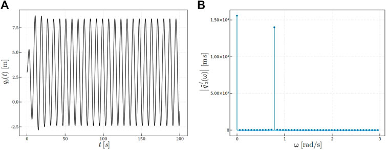
FIGURE 3. Free response (F₃(t) = 0): (A) $q_3^f\left(t\right)$; and (B) ${\widehat{q}}_3^f\left(\omega \right)$.

FIGURE 4

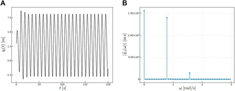
FIGURE 4. Response: (A) $q_3\left(t\right)$; and (B) ${\widehat{q}}_3\left(\omega \right)$.

Figure 5 shows the response difference $\mathrm{\Delta }{q}_3(t)=q_3(t)-q_3^f(t)$ and its Fourier transform ${\widehat{\mathrm{\Delta }q}}_3(\omega )$ on the domain in which the difference Δq₃(t) becomes almost stabilized, meaning the transient component almost vanishes.

FIGURE 5

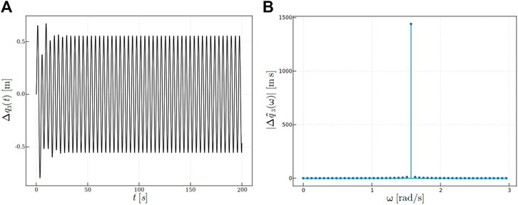
FIGURE 5. Response difference: (A) $\mathrm{\Delta }{q}_3\left(t\right)$; and (B) ${\widehat{\mathrm{\Delta }q}}_3\left(\omega \right)$.

Now, when comparing the reference solution, obtained by the reference analytical model ${\tilde{A}}_{33}=-1.4848+1.0221i$, to the one obtained from the learnt model ${\tilde{A}}_{33}=-1.5242+0.9823i$ (at principal frequency), an excellent accuracy can be noticed.

3.2 rNN and LSTM time simulations in both the linear and the nonlinear settings

In this section, we consider again the 3-mass dynamical system. The dynamical problem is integrated numerically to obtain the ground truth, that is, the reference solution. The computed data will be used for training the different neural networks, the rNN and the LSTM.

In both cases, the input data consist of the force F₃ and position q₃ in the previous time steps, which results in the surrogate $\mathcal{H}$:

${\tilde{q}}_3^i=\mathcal{H}\left(\left(\begin{array}{c}\hfill F_3^i\hfill \\ \hfill F_3^{i-1}\hfill \\ \hfill ⋮\hfill \\ \hfill F_3^{i-n+1}\hfill \end{array}\right),\left(\begin{array}{c}\hfill q_3^{i-1}\hfill \\ \hfill q_3^{i-2}\hfill \\ \hfill ⋮\hfill \\ \hfill q_3^{i-n}\hfill \end{array}\right)\right),(37)$

where ${\tilde{q}}_3^i$ is the prediction of q₃ at time step i.

As Eq. 37 reflects, different memory lengths from the use of the positive integer n, (n ≥ 0), are taken into account. For n ≠ 0, an initialization issue occurs.

In the case considered here, the larger memory is the toll ignoring the internal forces take, whose consequences on the observed variables are learnt from the time evolution of the last.

The initialization can be carried out following two routes:

• If we are interested in the forced regime, the long-time solution does not depend on the initialization.

• Should we prefer obtaining the transient solution, one could consider a coarser model that updates the state from the just previous state until completing the first n values. Then, the LSTM can take over.

In the present study, as previously indicated, we are focused on proving under which conditions a model relating observable inputs and outputs exists, despite the existence of hidden dynamics, resulting in a noticeable larger memory. For that reason, in the simulations considered in the present study, we assumed the first n values known.

3.2.1 Using a simple recurrent neural network

First, we consider a rNN surrogate model with n = 2, with respect to Eq. 37. The considered data for training come from the integration of the dynamical system, in both the linear and nonlinear cases.

The data consist of 10,000 states of the observable variables (coming as indicated from the standard integration of the dynamical system). These data are divided into two sets, the training and the testing ones, the former containing 80% of the points and the latter the remaining 20%.

The rNN consists of a single layer with one output ${\tilde{q}}_3^i$, in reference to Eq. 37. The network parameters and the initialization choices are the ones reported in Glorot and Bengio (2010). The algorithm is trained during 1,500 epochs, even though the use of fewer epochs leads to similar results.

The linear problem considers, once more: m₁ = m₂ = m₃ = 0.5Kg, c = 0.8 N/m, k₁ = k₂ = k₃ = 1 N/m, and l₁ = l₂ = l₃ = 1 m, expressing the applied loading the following way:

$\left\{\begin{array}{c}{F}_1\left(t\right)=2\hspace{0.17em}\cos \left(2\pi t\right)\hfill \\ F_2\left(t\right)=2\hspace{0.17em}\cos \left(\frac{\pi }{4}t\right)\hfill \\ F_3\left(t\right)=\frac{t}{t_{\max }}+\cos \left(\frac{\pi }{2}t\right)\hfill \end{array}\right.,(38)$

with t_max = 500s. This loading is used to generate the synthetic data that will serve afterward to identify the model q₃(t) as a function of the observed load F₃(t). During the training process of that model, F₂(t) and F₃(t) are again completely neglected.

The computed results from the trained network are given in Figure 6, being the mean absolute percentage errors (MAPE) 1.38% on the training set and 2.18% in the testing set.

FIGURE 6

FIGURE 6. Prediction of the observable position ${\tilde{q}}_3(t)$ computed from a trained rNN with n = 2 (colors green and red mark the training and testing sets, respectively). It can be noted that the blue curve is not visible because it is almost exactly under the green and red curves.

The same rNN (now with n = 3 in reference to Eq. 37) was employed to tackle a nonlinear dynamical system, with similar parameters to the ones considered in the linear case, except in what concerns the stiffnesses of the springs, now given by

$\left\{\begin{array}{c}{k}_1=k_{01}\left(1+\alpha \mathrm{\Delta }{l}_1\right)\hfill \\ k_2=k_{02}\left(1+\alpha \mathrm{\Delta }{l}_2\right)\hfill \\ k_3=k_{03}\left(1+\alpha \mathrm{\Delta }{l}_3\right)\hfill \end{array}\right.,(39)$

with k₀₁ = k₀₂ = k₀₃ = 10 N/kg and α = 10^–4 m⁻¹ (arbitrary, though carefully tuned to maintain the stability of the simulation) and where Δl_• is the elongation of the corresponding spring, i.e., Δl₂ = q₂ − q₁ − f₂, Δl₃ = q₃ − q₂ − f₃, and Δl₁ = q₁ − l₁.

The considered loading reads

$\left\{\begin{array}{c}{F}_1\left(t\right)=2\hspace{0.17em}\cos \left(2\pi t\right)\hfill \\ F_2\left(t\right)=2\hspace{0.17em}\cos \left(\frac{\pi }{4}t\right)\hfill \\ F_3\left(t\right)=\cos \left(\frac{\pi }{2}t\right)\hfill \end{array}\right..(40)$

The results concerning the nonlinear dynamical system are reported in Figure 7, and, for the sake of clarity, the associated absolute error is reported in Figure 8, with a mean absolute percentage error (MAPE) of 1.34% in the training set and 1.29% in the testing set. The error is slightly larger in the training set, probably due to the larger transient phase presenting higher peaks.

FIGURE 7

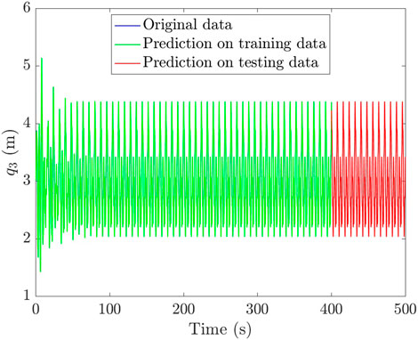
FIGURE 7. Prediction of the observable position ${\tilde{q}}_3(t)$ in the nonlinear case, computed by a trained rNN with n = 3 (again, colors refer to the training and testing sets). It can be noted that the blue curve is not visible because it is almost exactly under the green and red curves.

FIGURE 8

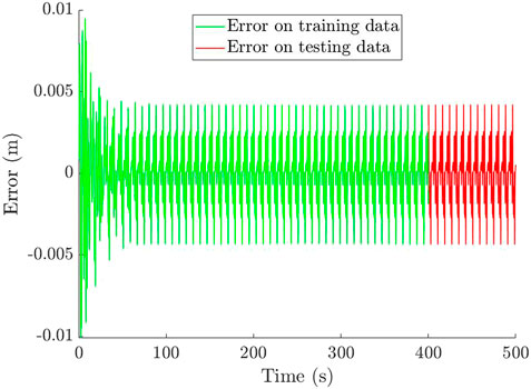
FIGURE 8. Error in the prediction of the observable position ${\tilde{q}}_3(t)$ in the nonlinear case, computed by a trained rNN with n = 2 (the same color code applies).

3.2.2 Using an LSTM recurrent neural network

The same linear and nonlinear dynamical systems are now processed by LSTM cells, with the same network parameters and initializations used for the rNN.

When addressing the linear case, the computed results are given in Figure 9, with an MAPE of 0.84% in the training set and 1.33% in the testing set. The results in the nonlinear case are reported in Figure 10, and again, for the sake of clarity, the associated absolute error is presented in Figure 11, presenting an MAPE of 0.15% in the training set and 0.14% in the testing set. The error is again slightly larger in the training set for the same reasons given before.

FIGURE 9

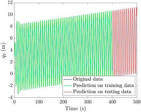
FIGURE 9. Prediction of the observable position ${\tilde{q}}_3(t)$ computed by a trained LSTM with n = 2 (the same color code is employed). It can be noted that the blue curve is not visible because it is almost exactly under the green and red curves.

FIGURE 10

FIGURE 10. Prediction of the observable position ${\tilde{q}}_3(t)$ in the nonlinear case, computed by a trained LSTM with n = 3 (same color code). It can be noted that the blue curve is not visible because it is almost exactly under the green and red curves.

FIGURE 11

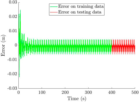
FIGURE 11. Error in the prediction of the observable position ${\tilde{q}}_3(t)$ in the nonlinear case, computed by a trained LSTM with n = 3 (same color code).

As expected, LSTM outperforms the rNN for a large number of epochs. It was noticed that by reducing the number of epochs, the rNN outperforms LSTMs because convergence is more easily achieved using a lower number of parameters. The error in the linear case was larger, possibly due to the fact that it involves close to zero values which negatively impacts the error calculation.

It must be noted that several experiments with various number of elements, different damping coefficients, stiffnesses, lengths, and masses have been carried out with similarly satisfactory results (MSE error always below 0.07 for both training and testing).

4 Conclusion

The issue related to the circumstances enabling the construction of a model relating the input and output of observed quantities, in the frame of a larger system involving a hidden state that affects the observed variables, was revisited in the present work.

We proved that for time-independent models, such a model exists, and the learnt model is the one where the hidden variables are condensed into the observed ones. As soon as the loading in the internal unresolved degrees of freedom does not change, the computed model can be reused for any other prediction with different loading in the observed region concerned by the learnt model.

In the transient case, the Fourier transform, applicable in the linear case far away from the transient regime, allowed to prove that such a model can be learnt, but in this case, the model involves the recent history of the considered variables (present and recent past) and remains valid for any loading in the observed region, as soon as the forces applied on the hidden part have the same Fourier transforms.

When operating in the time domain, the rNN and LSTM are demonstrably the most natural choices for performing the learning task, and it is also expected that they allow for addressing nonlinear dynamical systems. Regarding time-integration, the performances of both neural networks, rNN and LSTM, remain similar and prove that, as expected from the developments given in Section 2, the model relating observable inputs and outputs can be learnt as soon as past values of them are considered in the model construction.

Data availability statement

The datasets presented in this study can be found in online repositories. The names of the repository/repositories and accession number(s) can be found below: https://github.com/cghnatios/LSTM-rNN-for-Modeling-systems-from-partial-observations-.git.

Author contributions

VC contributed to the development of the analytical methodologies, VA, CG, LI-V, and SG performed the implementation of learning procedures, while FM, EC, and FC contributed to the global methodology and research development.

Funding

This research is also part of the DesCartes program and is supported by the National Centre for Scientific Research (CNRS), Prime Minister Office, Singapore under its Campus for Research Excellence and Technological Enterprise (CREATE) program. This study has received funding from the European Union Horizon 2020 research and innovation program under the Marie Skłodowska-Curie grant agreement No. 956401 (Project XS-Meta).

Acknowledgments

Authors acknowledge the contribution and support of the ESI-ENSAM research chair CREATE-ID. The support by the ESI Group through the ESI Chair at ENSAM Arts et Métiers Institute of Technology, and through the project 2019-0060 “Simulated Reality” at the University of Zaragoza is also acknowledged. The support of the Spanish Ministry of Science and Innovation, AEI /10.13039/501100011033, through Grant number PID2020-113463RB-C31 and by the Regional Government of Aragón, grant T24-20R, and the European Social Fund, are also gratefully acknowledged.

Conflict of interest

FC was employed by the company CNRS@CREATE LTD.

The remaining authors declare that the research was conducted in the absence of any commercial or financial relationships that could be construed as a potential conflict of interest.

Publisher’s note

All claims expressed in this article are solely those of the authors and do not necessarily represent those of their affiliated organizations, or those of the publisher, the editors, and the reviewers. Any product that may be evaluated in this article, or claim that may be made by its manufacturer, is not guaranteed or endorsed by the publisher.

References

Argerich, C., Carazo, A., Sainges, O., Petiot, E., Barasinski, A., Piana, M., et al. (2020). Empowering design based on hybrid twin: Application to acoustic resonators. Designs 4, 44. doi:10.3390/designs4040044

CrossRef Full Text | Google Scholar

Benabou, L. (2021). Development of lstm networks for predicting viscoplasticity with effects of deformation, strain rate, and temperature history. J. Appl. Mech. 88, 1–30. doi:10.1115/1.4051115

CrossRef Full Text | Google Scholar

Borzacchiello, D., Aguado, J., and Chinesta, F. (2019). Non-intrusive sparse subspace learning for parametrized problems. Arch. Comput. Methods Eng. 26, 303–326. doi:10.1007/s11831-017-9241-4

CrossRef Full Text | Google Scholar

Bronstein, M. M., Bruna, J., Cohen, T., and Velivckovi’c, P. (2021). Geometric deep learning: Grids, groups, graphs, geodesics, and gauges. ArXiv abs/2104.13478.

Google Scholar

Brunton, S. L., and Kutz, J. N. (2019). Data-driven science and engineering: Machine learning, dynamical systems, and control. Cambridge University Press. doi:10.1017/9781108380690

CrossRef Full Text | Google Scholar

Chinesta, F., Ladeveze, P., and Cueto, E. (2011). A short review on model order reduction based on proper generalized decomposition. Arch. Comput. Methods Eng. 18, 395–404. doi:10.1007/s11831-011-9064-7

CrossRef Full Text | Google Scholar

Chinesta, F., Leygue, A., Bordeu, F., Aguado, J. V., Cueto, E., Gonzalez, D., et al. (2013). Pgd-based computational vademecum for efficient design, optimization and control. Arch. Comput. Methods Eng. 20, 31–59. doi:10.1007/s11831-013-9080-x

CrossRef Full Text | Google Scholar

Chinesta, F., Keunings, R., and Leygue, A. (2014). The proper generalized decomposition for advanced numerical simulations: A primer. Springer. doi:10.1007/978-3-319-02865-1

CrossRef Full Text | Google Scholar

Chinesta, F., Huerta, A., Rozza, G., and Willcox, K. (2015). The encyclopedia of computational mechanics. in Chap. Model order reduction (John Wiley & Sons), 1–36.

Google Scholar

Chinesta, F., Cueto, E., Abisset-Chavanne, E., Duval, J. L., and Khaldi, F. E. (2020). Virtual, digital and hybrid twins: A new paradigm in data-based engineering and engineered data. Arch. Comput. Methods Eng. 27, 105–134. doi:10.1007/s11831-018-9301-4

CrossRef Full Text | Google Scholar

Fasel, U., Kutz, J. N., Brunton, B. W., and Brunton, S. L. (2022). Ensemble-sindy: Robust sparse model discovery in the low-data, high-noise limit, with active learning and control. Proc. Math. Phys. Eng. Sci. 478, 20210904. doi:10.1098/rspa.2021.0904

PubMed Abstract | CrossRef Full Text | Google Scholar

Ghanem, R., Soize, C., Mehrez, L., and Aitharaju, V. (2022). Probabilistic learning and updating of a digital twin for composite material systems. Int. J. Numer. Methods Eng. 123, 3004–3020. doi:10.1002/nme.6430

CrossRef Full Text | Google Scholar

Glorot, X., and Bengio, Y. (2010). “Understanding the difficulty of training deep feedforward neural networks,”. Proceedings of the thirteenth international conference on artificial intelligence and statistics. Editors Y. W. Teh, and M. Titterington (Chia Laguna Resort, Sardinia, Italy: Proceedings of Machine Learning Research), 9, 249–256.

Google Scholar

González, D., Chinesta, F., and Cueto, E. (2021). Learning non-markovian physics from data. J. Comput. Phys. 428, 109982. doi:10.1016/j.jcp.2020.109982

CrossRef Full Text | Google Scholar

Goodfellow, I., Bengio, Y., and Courville, A. (2016). Deep learning. MIT Press. Available at: http://www.deeplearningbook.org.

Google Scholar

Hernandez, Q., Badias, A., Chinesta, F., and Cueto, E. (2022). Thermodynamics-informed graph neural networks. IEEE Trans. Artif. Intell., 1. doi:10.1109/TAI.2022.3179681

CrossRef Full Text | Google Scholar

Hinton, G., and Zemel, R. (1993). “Autoencoders, minimum description length and helmholtz free energy,” in Advances in neural information processing systems, Denver, CO, USA (Morgan-Kaufmann.), 6, 3–10.

Google Scholar

Hochreiter, S., and Schmidhuber, J. (1997). Long short-term memory. Neural Comput. 9, 1735–1780. doi:10.1162/neco.1997.9.8.1735

PubMed Abstract | CrossRef Full Text | Google Scholar

Ibáñez, R., Abisset-Chavanne, E., Ammar, A., González, D., Cueto, E., Huerta, A., et al. (2018). A multidimensional data-driven sparse identification technique: The sparse proper generalized decomposition. Complexity 2018, 1–11. doi:10.1155/2018/5608286

CrossRef Full Text | Google Scholar

Kapteyn, M. G., and Willcox, K. E. (2020). From physics-based models to predictive digital twins via interpretable machine learning. ArXiv abs/2004.11356. doi:10.48550/ARXIV.2004.11356

CrossRef Full Text | Google Scholar

Lee, K., and Carlberg, K. T. (2020). Model reduction of dynamical systems on nonlinear manifolds using deep convolutional autoencoders. J. Comput. Phys. 404, 108973. doi:10.1016/j.jcp.2019.108973

CrossRef Full Text | Google Scholar

Liu, Z., and Tegmark, M. (2021). Machine learning conservation laws from trajectories. Phys. Rev. Lett. 126, 180604. doi:10.1103/PhysRevLett.126.180604

PubMed Abstract | CrossRef Full Text | Google Scholar

Luo, H., Huang, M., and Zhou, Z. (2018). Integration of multi-Gaussian fitting and lstm neural networks for health monitoring of an automotive suspension component. J. Sound Vib. 428, 87–103. doi:10.1016/j.jsv.2018.05.007

CrossRef Full Text | Google Scholar

Makhzani, A., and Frey, B. J. (2014). k-sparse autoencoders. CoRR abs/1312.5663. doi:10.48550/ARXIV.1312.5663

CrossRef Full Text | Google Scholar

Manohar, K., Kutz, J. N., and Brunton, S. L. (2018). Optimal sensor and actuator placement using balanced model reduction. ArXiv abs/1812.01574.

Google Scholar

Moya, B., Badías, A., Alfaro, I., Chinesta, F., and Cueto, E. (2022b). Digital twins that learn and correct themselves. Int. J. Numer. Methods Eng. 123, 3034–3044. doi:10.1002/nme.6535

CrossRef Full Text | Google Scholar

Moya, B., Badias, A., González, D., Chinesta, F., and Cueto, E. (2022a). Physics-informed reinforcement learning for perception and reasoning about fluids. ArXiv abs/2203.05775. doi:10.48550/ARXIV.2203.05775

CrossRef Full Text | Google Scholar

Ng, A. (2011). Sparse autoencoder. CS294A Lecture notes. Tech. rep. Stanford university.

Google Scholar

Sancarlos, A., Cameron, M., Abel, A., Cueto, E., Duval, J.-L., and Chinesta, F. (2021a). From rom of electrochemistry to ai-based battery digital and hybrid twin. Arch. Comput. Methods Eng. 28, 979–1015. doi:10.1007/s11831-020-09404-6

CrossRef Full Text | Google Scholar

Sancarlos, A., Cameron, M., Le Peuvedic, J.-M., Groulier, J., Duval, J.-L., Cueto, E., et al. (2021b). Learning stable reduced-order models for hybrid twins. Data-Centric Eng. 2, e10. doi:10.1017/dce.2021.16

CrossRef Full Text | Google Scholar

Sancarlos, A., Champaney, V., Duval, J. L., Cueto, E., and Chinesta, F. (2021c). Pgd-based advanced nonlinear multiparametric regressions for constructing metamodels at the scarce-data limit. ArXiv abs/2103.05358.

Google Scholar

Schmidhuber, J. (2015). Deep learning in neural networks: An overview. Neural Netw. 61, 85–117. doi:10.1016/j.neunet.2014.09.003

PubMed Abstract | CrossRef Full Text | Google Scholar

Tuegel, E. J., Ingraffea, A. R., Eason, T. G., and Spottswood, S. M. (2011). Reengineering aircraft structural life prediction using a digital twin. Int. J. Aerosp. Eng. 2011, 1–14. doi:10.1155/2011/154798

CrossRef Full Text | Google Scholar

Venkatesan, R., and Li, B. (2017). Convolutional neural networks in visual computing: A concise guide. London, United Kingdom: CRC Press.

Google Scholar

Weiss, K., Khoshgoftaar, T. M., and Wang, D. (2016). A survey of transfer learning. J. Big Data 3, 9. doi:10.1186/s40537-016-0043-6

CrossRef Full Text | Google Scholar

Williams, J., Zahn, O., and Kutz, J. N. (2022). Data-driven sensor placement with shallow decoder networks. arXiv. doi:10.48550/ARXIV.2202.05330

CrossRef Full Text | Google Scholar

Zhou, G.-B., Wu, J., Zhang, C.-L., and Zhou, Z.-H. (2016). Minimal gated unit for recurrent neural networks. Int. J. Autom. Comput. 13, 226–234. doi:10.1007/s11633-016-1006-2

CrossRef Full Text | Google Scholar