 Victor M. Lopez-Hirata1*
 Cristobal R. Escamilla-Illescas1*Rodrigo Calva-Luna1Maribel L. Saucedo-Muñoz1Erika O. Avila-Davila2Jose D. Villegas-Cardenas1
- 1Department of Metallurgy and Materials, Instituto Politecnico Nacional, Mexico City, Mexico
- 2Tecnologico Nacional de Mexico/Instituto Tecnológico de Pachuca, DEPI, Pachuca, Mexico
- 3Universidad Politecnica del Valle de Mexico, Mexico City, Mexico
The phase decomposition of hypothetic A–B–C alloys was analyzed using the phase-field method based on the numerical solution of the Cahn–Hilliard equation. The effect of the interaction parameters on the growth kinetics of phase decomposition was also studied. The results indicated that the driving force was the fastest if all the three interaction parameters were equal, promoting the quickest growth kinetics of the ternary alloy. The phase decomposition occurred spinodally and caused the formation of three phases, A-rich, B-rich, and C-rich. In this case, the spinodal curve formed an isolated island. If one or two interaction parameters are equal to zero, the growth kinetics is slower. This condition originated only the formation of two decomposed phases with the chemical composition of either one element or two elements depending on the interaction parameters. Likewise, the spinodal curve is not completely located within the isothermal section.
Introduction
A microstructure is defined as a spatial array of phases with different chemical compositions, possible crystalline defects, and crystalline structures (Biner, 2017). Most of the mechanical properties of engineering materials are closely related to their microstructure.
A common strengthening mechanism of engineering alloys is a dispersed fine second phase in the matrix (Provatas and Elder, 2010), that is, the morphology, size and size distribution, and volume fraction of the second phase play an essential role in the mechanical properties (Janssens et al., 2007). The microstructure of an alloy is strongly determined by its chemical composition and manufacturing processes, such as casting and melting, heat treatment, welding, and thermomechanical treatment. During all these processes and service operation of industrial components, this microstructure changes due to the external fields of temperature, stress, or magnetic to decrease the total free energy, involving chemical, interfacial, or magnetic energies. The thermodynamics and kinetics of phase transformations control the microstructure evolution of alloys. Due to the complex nature of the microstructure, different numerical methods have been applied (Chen, 2002; Jannsens et al., 2007) to solve the equations that describe the microstructure evolution. This type of problem has been treated using sharp interface modeling; however, the complete description of the interfaces between compositional or structural domains is complex in two or three dimensions. Therefore, based on the diffuse interface modeling, the phase-field method has emerged (Chen, 2002) as a good alternative for microstructure simulation. The phase-field method has successfully simulated different phase transformations (Chen, 1994; Steinbach, 2009; Muramatsu et al., 2010; Ansari et al., 2021; Lee et al., 2021), such as dendritic growth, spinodal decomposition, recrystallization, and coarsening of precipitates. Most of these works were conducted in pure metals or binary alloys. Nevertheless, the industrial alloys are usually multicomponents, and thus, it is necessary to pursue the analysis of phase transformations for multicomponent alloys using the phase-field method.
For instance, several studies (Avila-Davila et al., 2009; Eidenberger et al., 2010; Du et al., 2016; Kim et al., 2020; Mianroodi et al., 2021) applied the phase-field method to spinodal decomposition either for hypothetic or real binary and ternary alloys. Most spinodal decomposition simulations (Suwa et al., 2002; Avila et al., 2012) usually considered constant mobility or diffusivity for binary alloys. In contrast, nearly equal diffusivities of components seem to be reasonable for multicomponent alloys but not in the case of simulation for minerals (12). Moreover, several theoretical studies focused on explaining the spinodal decomposition for ternary and multicomponent systems (De Fontaine, 1972; De Fontaine, 1973; Hoyt, 1989; Petrishcheva and Abart, 2012). De Fontaine (1972) pointed out the spinodal decomposition without strain energy effect even for significant differences in atomic sizes of the components.
Moreover, several ternary alloy systems, such as Cu–Ni–Fe, Cu–Ni–Cr, Al–Zn–Cu, Fe–Cr–Co, and Fe–Cr–Ni (Lopez-Hirata et al., 1993; Kuwano et al., 1996; Lopez-Hirata et al., 2001; Mukhamedov et al., 2017), base their good mechanical or magnetic properties on the spinodal decomposition process. Thus, the analysis of the effect of different interaction parameter values for a regular solution model on the growth kinetics of phase decomposition of hypothetic A–B–C ternary alloys is an essential issue in understanding the microstructure developed after the aging treatment of ternary alloys. This study enables us to compare the kinetic and microstructure results for different thermodynamic behavior of ternary alloy systems. These results can explain the main difference in the phase decomposition of the real alloy systems.
Therefore, the present work aims to conduct the thermodynamic and kinetic analyses of spinodal decomposition for hypothetic ternary A–B–C alloys to obtain more details of the phase decomposition for different ternary alloy systems according to their thermodynamic behavior.
Numerical Methodology
Equilibrium Ternary Phase Diagrams
The regular solid solution model for a ternary alloy can be expressed by the following equation (Meijering, 1950; Meijering, 1951; Nisizawa, 2008):
where XA, XB, and XC are the mole fraction of elements A, B, and C, respectively;
The miscibility gap for a ternary system is also determined by deriving Eq. 1 with respect to the composition, equating to zero, and solving the generated simultaneous nonlinear equation system. For instance, considering the first-order partial derivatives
These are only one-third of the solution for a given temperature; however, the complete solution is reached after solving the other two pairs of simultaneous equations.
The saddle points define the spinodal surface of the ternary system by the following second or partial derivatives with respect to composition:
By applying these equations to Eq. 1, the following quadratic equation is determined:
There are other two equations of this type, and they are solved for the spinodal temperature T considering a specific alloy composition. Table 1 shows the simulated conditions for the spinodal curve and miscibility gap for the hypothetic ternary A–B–C system.

TABLE 1. Simulation conditions for the hypothetic A–B–C spinodal curve and miscibility gap at 800 K.
Phase-Field Modeling
The phase-field method was based on a solution of the Cahn–Hilliard equation for multicomponent alloys (Chen, 1994; Chen, 2002; Avila-Davila et al., 2009; Kim et al., 2020):
where
where
and
where
In the case of a ternary alloy, the Cahn–Hilliard equation, Eq. 8, has to be solved twice, according to the following equations:
The concentration
Results
Miscibility Gap and Spinodal Curve
Figures 1A–C illustrate the miscibility gap, free energy curve at 900 K, and the spinodal curve of the A–B–C alloy system, respectively, for the following interaction parameters,
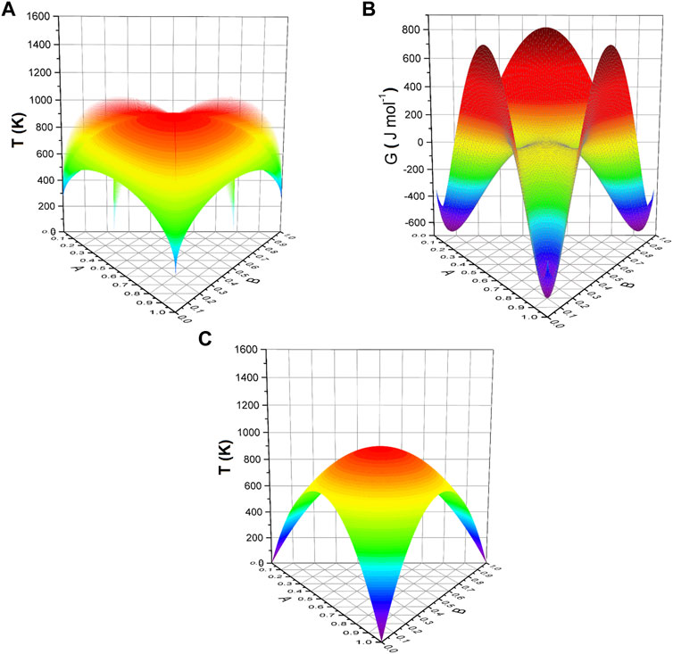
FIGURE 1. (A) Miscibility gap, (B) free energy curve, and (C) spinodal curve for the A–B–C alloy system, respectively, for
The maximum temperature of the miscibility gap increases with the interaction parameters, and thus the aging for phase separation can be conducted at higher temperatures.
Figures 2A–C show the isothermal sections of ternary A–B–C phase diagrams at 600, 800, and 1000 K, respectively, for
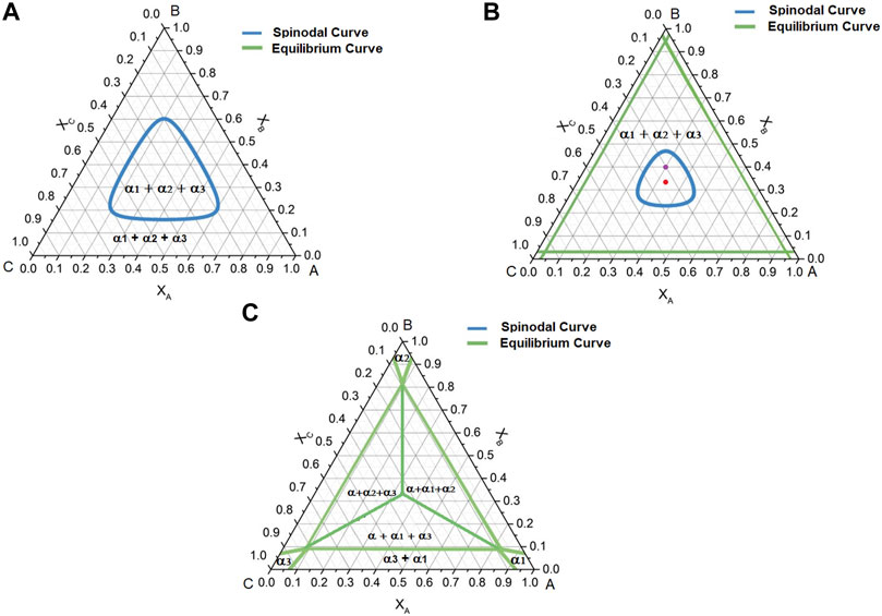
FIGURE 2. Isothermal sections of the miscibility gap and spinodal curve for the A–B–C alloy system with
The isothermal sections of ternary phase diagrams at 600, 800, and 1000 K are shown in Figures 3A–C, respectively, for
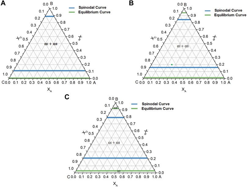
FIGURE 3. Isothermal sections of the miscibility gap and spinodal curve for the A–B–C alloy system with
Figures 4A–C present the isothermal sections of ternary phase diagrams at 600, 800, and 1000 K in Figures 3A–C, respectively, for
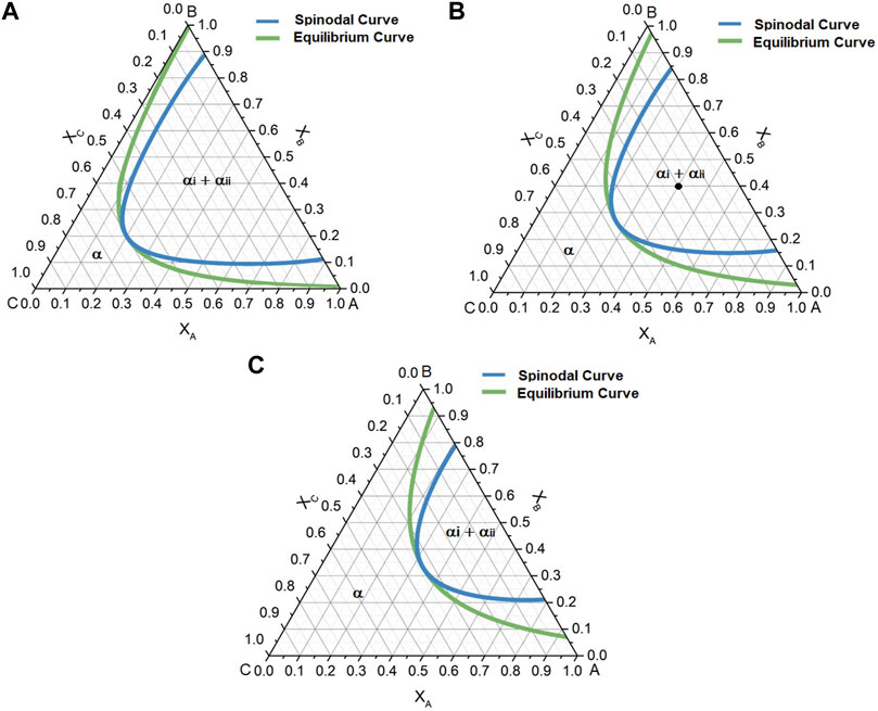
FIGURE 4. Isothermal sections of the miscibility gap and spinodal curve for the A–B–C alloy system with
All calculated equilibrium ternary phase diagrams and spinodal curves are in good agreement with those reported in the literature (Meijering, 1950; Meijering, 1951; Nisizawa, 2008).
Concentration Profiles and Microstructure Evolution
The phase-field simulated evolution of A, B, and C concentration profiles and microstructure evolution with time during aging at 800 K are shown in Figures 5, 6A–D, respectively, for an alloy composition of XA =XB = Xc= ⅓ for case I, as indicated by a red point in Figure 2B. The concentration profiles of the supersaturated solution, 0 s, present a random concentration fluctuation for the A, B, and C elements. The formation of low amplitude concentration modulation is observed in the case of aging for 10 s. However, the modulation amplitude increases for the aging of 30 s, which confirms that the phase separation takes place by the spinodal decomposition mechanism. Moreover, this concentration profile clearly shows the decomposition of the supersaturated solid solution into a mixture of A-rich α1, B-rich α2, and C-rich α3 phases. Likewise, this plot also indicates the coalescence of some of the composition fluctuation for times longer than 30 s.
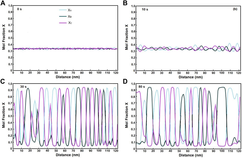
FIGURE 5. Simulated concentration profiles of the A–B–C alloy for case I with XA = XB = Xc= ⅓ aged at 800 K for (A) 0 s, (B) 10 s, (C) 30 s, and (D) 80 s.
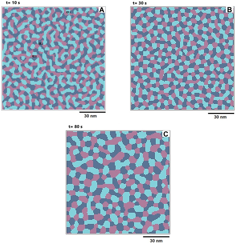
FIGURE 6. Simulated microstructure of the A–B–C alloy for case I with XA =XB = Xc= ⅓ aged at 800 K for (A) 10 s, (B) 30 s, and (C) 80 s.
In the microstructure evolution, the presence of interconnected A-rich α1, B-rich α2, and C-rich α3 phases is observed in Figure 6A. This type of microstructure is designated as an interconnected modulated or mottled structure, and it is characteristic of the early stages of spinodal decomposition (Cahn, 1961; Cahn, 1968; Morral, 1971). As aging progresses, the spinodally decomposed phases become equiaxial, and their sizes continue increasing with time up to 80 s. However, the volume fraction of each decomposed phase is approximately the same and consistent with the alloy composition.
Figures 7A–D show the evolution of concentration profiles for the ternary alloy for case II with a composition of XA = 0.3, XB = 0.4, and Xc = 0.3, as shown by a violet point in Figure 2B, aged at 800 K at different times. In this case, The A and C concentration profiles are almost overlapped for aging of 10 s, as shown in Figure 7A. The evolution of concentration profiles shows the presence of the three decomposed A-rich, B-rich, and C-rich phases after aging for 30 s, as shown in Figure 7B, which is more notorious after aging for 80 s. Even more, the coalescence of composition fluctuations is clearly observed after aging for 80 s for the B concentration profile, as shown in Figure 7C. The modulation amplitude also increases with time, which confirms spinodal decomposition. In contrast, the microstructure evolution with time is shown for the same case II in Figures 8A–C. Figure 8A shows percolated structure of the three decomposed phases. This morphology changes to equiaxial, and the size increases with the aging time. According to the alloy composition, the volume fraction of the B-rich α2 phase is slightly higher than that of the other two phases.
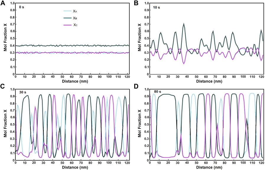
FIGURE 7. Simulated concentration profiles of the A–B–C alloy for case II with XA = 0.3, XB = 0.4, and Xc = 0.3 aged at 800 K for (A) 0 s, (B) 10 s, (C) 30 s, and (D) 80 s.
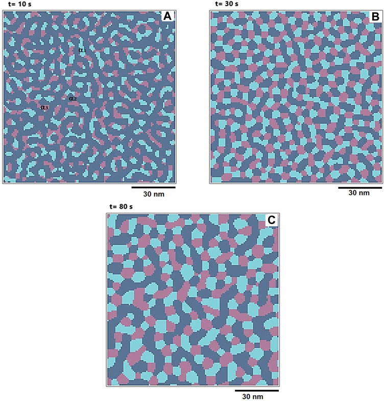
FIGURE 8. Simulated microstructure of the A–B–C alloy for case II with XA = 0.3, XB = 0.4, and Xc = 0.3 aged at 800 K for (A) 10 s, (B) 30 s, and (C) 80 s.
The simulated concentration profiles of A–B–C alloy for case III with XA = 0.25, XB = 0.20, and Xc = 0.5, the green point in Figure 3B, aged at 800 K are shown in Figures 9A–D for 0, 10, 30, and 80 s, respectively. This composition was selected to analyze the phase decomposition close to the spinodal line. In this case, the phase decomposition occurs again spinodally, since the modulation amplitude increases with time. Nevertheless, the supersaturated solid solution decomposes into a mixture of A–C rich αI and B-rich αII phases with the B content almost constant for the two phases, which is attributable to
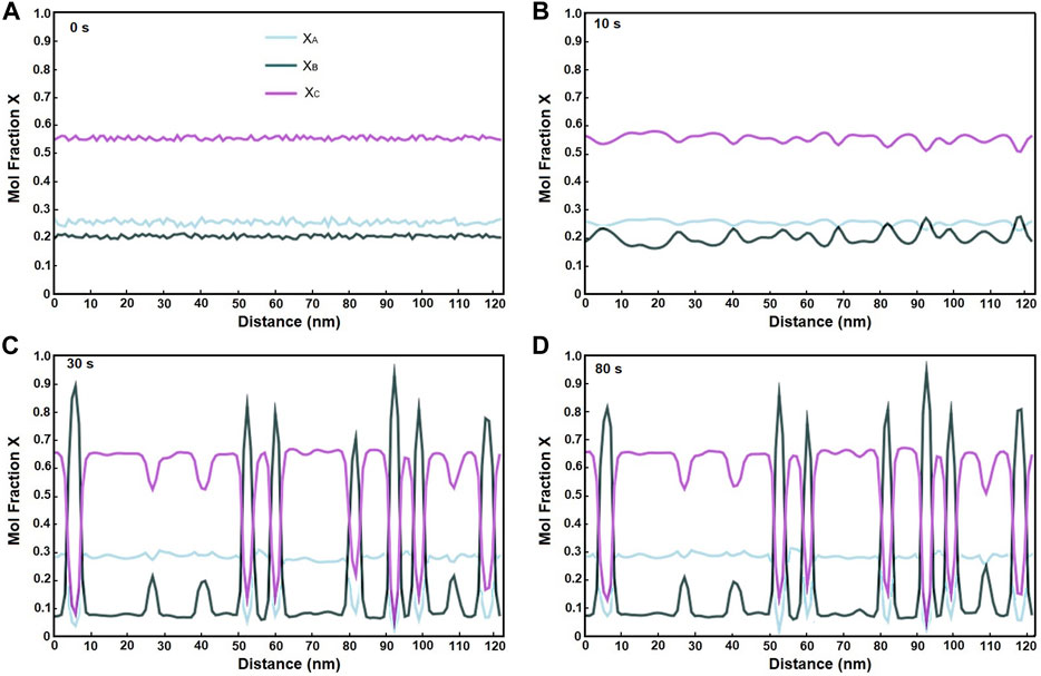
FIGURE 9. Simulated concentration profiles of the A–B–C alloy for case III with XA = 0.25, XB = 0.20, and Xc = 0.55 aged at 800 K for (A) 0 s, (B) 10 s, (C) 30 s, and (D) 80 s.
The simulated microstructure of A–B–C alloy for case III is shown in Figures 10A–D. The simulated micrographs show the presence of two A–C rich αI and B-rich αII phases. Furthermore, the predominant phase is the A–C rich, which is consistent with the alloy composition. Another interesting characteristic is that the phase morphology of B-rich is like cuboids, and it resembles a precipitation process instead of spinodal decomposition. This behavior can be attributed to the fact that the alloy composition is near the miscibility gap and spinodal line.
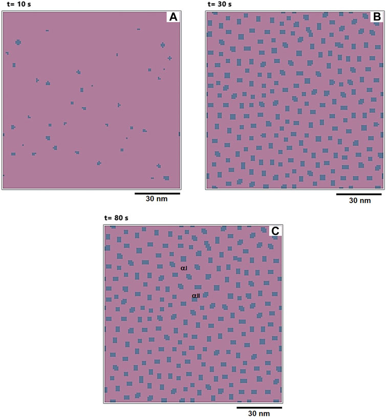
FIGURE 10. Simulated microstructure of the A–B–C alloy for case III with XA = 0.25, XB = 0.20, and Xc = 0.55 aged at 800 K for (A) 10 s, (B) 30 s, and (C) 80 s. s
The evolution of concentration profiles of the aged ternary alloy with XA = 0.40, XB = 0.40, and Xc = 0.20 for case IV, as indicated by the black point in Figure 4B, aged at 800 K is shown in Figures 11A–D for 10 s, 30, and 80 s, respectively. This evolution clearly shows that the supersaturated solid solution decomposes spinodally into a mixture of A-rich αi and B-rich αii phases with an almost constant C content.
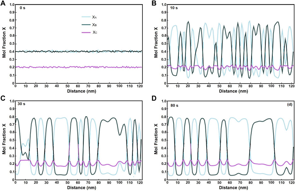
FIGURE 11. Simulated concentration profiles of the A–B–C alloy for case IV with XA = 0.40, XB = 0.40, and Xc = 0.20 aged at 800 K for (A) 0 s, (B) 10 s, (C) 30 s, and (D) 80 s.
The microstructure evolution for case IV is illustrated in Figures 12A–C. This microstructure evolution shows that the spinodal decomposition produces a mixture of A-rich αi and B-rich αii phases. These phases have a percolated structure and increase their size with time; however, the morphology shows no change with time.
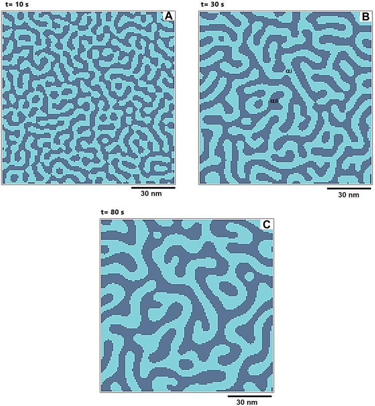
FIGURE 12. Simulated microstructure of the A–B–C alloy for case IV with XA = 0.40, XB = 0.40, and Xc = 0.20 aged at 800 K for (A) 10 s, (B) 30 s, and (C) 80 s.
Discussion
Growth Kinetic of Phase Decomposition
The simulation time for the present study is very short. Thus, the present work results can be analyzed by considering the linear Cahn–Hilliard theory of spinodal decomposition (Cahn, 1961; Cahn, 1968). The modified diffusion equation for spinodal decomposition is given by:
The variables of this equation have the same meaning as in Eq. 8, and it has the following analytical solution:
where R(β) is the amplification factor, r is the position vector, β is the wave number (2π/λ), and λ is the modulation wavelength.
The amplification factor R(β) is given by the following equation:
As it is well known, if R(β) > 0, any composition fluctuations will grow, while any fluctuations will decay if R(β) < 0. To have positive values, it is necessary that the alloy composition co is within the spinodal curve where
βm is defined as follows:
The variation of modulation wavelength λ versus aging time t is shown in Figure 13 for the four cases of the present work. In all cases, the growth kinetics of modulation wavelength with time is very slow, i.e., almost constant. Furthermore, if a power law, λ = ktn, is considered, the time exponent n was determined to be about 0.02–0.05. According to the linear Cahn–Hilliard theory of spinodal decomposition (Cahn, 1961; Kostorz, 1992), this behavior is a characteristic of the spinodal decomposition at the early stages. Monte Carlo simulations (Binder et al., 1974; Binder et al., 1976; Kostorz, 1992) have shown that the time exponent n is between 0.16 and 0.25, associated with cluster coagulation. Although the linearized spinodal decomposition theory is not rigorously followed, this theory will be used to explain the present work results qualitatively.
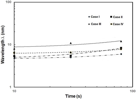
FIGURE 13. Plot of modulation wavelength λ versus time t for the present study cases.
For instance, the alloy composition for case I is located at the center of the miscibility gap, and thus the driving force,
In the case of the modulation amplitude, the highest value of R(β) is expected for the alloy composition of case I, in comparison to that for case II; however, the modulation amplitude for 10 s, as shown in Figure 6B, is lower than that of case II, as shown in Figure 8B, that is, somehow, R(β) must be higher for case II. The spinodal decomposition theory for ternary alloys (Morral et al., 1971) states that the diffusion coefficients D or mobilities M play an important role in the growth kinetics of spinodal decomposition. In case I, the mole fraction is the same for A, B, and C, which promotes that the composition fluctuations grow in the same way. However, in case II, the B element is dominant, and thus the composition fluctuation grows more rapidly. This fact suggests that the mobility MBB may cause a higher amplification factor R(β) and then faster growth kinetics.
The modulation amplitude for cases III and IV is more significant than that of previous cases. This fact suggests that the amplification factor R(β) is higher than that in previous cases. This high value can be attributed to faster mobility since one or two interaction parameters are zero. Nevertheless, the modulation fluctuation of the highest element mole fraction is dominant during the phase decomposition.
The evolution of concentration profiles with time is in good agreement with the expected behavior reported in the literature (De Fontaine, 1972; Maier-Paape, 2000). If the initial alloy composition in the three-phase field is almost equal for the three components, the evolution of concentration profiles with time consists of two dominating profiles from the binary alloy case, which leads to the formation of three A-, B-, and C-rich phases. For different alloy compositions, located out of the three phase-fields, only one dominating profile of the binary determines the formation of two phases.
Phase Decomposition of Ternary Alloys
The present calculation is based on a regular solution model of hypothetic ternary alloys without considering elastic-strain energy or other effects, such as magnetism. These factors must be included in Eq. 1. Moreover, the regular solution model, used for the present work, only permits the inclusion of first-order interactions. The Redlick–Kister equation (Nishizawa T., 2008) is a sub-regular model, which provides for higher-order interactions, and it is used for the solution modeling of industrial alloys. Figures 14A,B show the Calphad-calculated equilibrium phase diagrams for Cu–Ni–Fe and Fe–Cr–Co alloys (Thermo-Calc, 2022). These diagrams correspond to those presented in Figures 3, 4. The type of miscibility gap of the equilibrium diagram is like the calculated one. However, some differences in the phase regions originated because the interaction parameter is not the same for the different thermodynamic interactions in the real alloy system as used for the hypothetic A–B–C alloys.
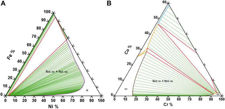
FIGURE 14. Calphad-calculated equilibrium phase diagrams for (A) Cu–Ni–Fe and (B) Fe–Cr–Co alloy systems.
This paragraph compares qualitatively the present study cases with either the calculated or experimental results of actual ternary alloys reported in the literature (Kuwano et al., 1996; Miller et al., 1996; Suwa et al., 2002; Avila-Davila et al., 2009; Lopez-Hirata et al., 2017). For instance, the Al-20at.%Zn-10at.%Cu alloy has been reported (Lopez-Hirata et al., 2017) to have the spinodal decomposition of an fcc supersaturated solid solution into a mixture of fcc Cu-rich Al–Zn and Cu-poor Al–Zn phases after aging at 450°C at different times. This alloy system has an interaction parameter
Conclusion
Thermodynamic and kinetic analyses of the spinodal decomposition were conducted for hypothetic ternary alloys, and the conclusions are summarized as follows:
1 The fastest spinodal decomposition took place for the alloy composition at the center of the miscibility gap and all interaction parameters with an equal value of 25,000 J/mol because of the highest driving force for phase decomposition. The phase decompositions involved the formation of the same volume fraction of three phases, A-rich α1, B-rich α2, and C-rich α3.
2 All the other cases when one or two interaction parameters are equal to zero promote slower kinetics of phase decomposition, which is attributed to the lower driving force, and involve the formation of two decomposed phases. The composition of decomposed phases is mainly associated with one or two components.
3 The values of interaction parameters are related to three types of miscibility gaps and spinodal curves, which can correspond to different real alloy systems. These values defined the equilibrium phase composition.
Data Availability Statement
The raw data supporting the conclusion of this article will be made available by the authors, without undue reservation.
Author Contributions
VL-H, MS-M, and EA-E conceptualized the idea. CE-I and RC-L developed computer programs. VL-H, CE-I, and RC-L performed the simulations. VL-H, JV-C, and MS-M drafted the manuscript. All authors contributed to the manuscript and agreed to the submitted version.
Funding
This work was supported as part of a Conacyt Research Project, A1-S-9682. The authors wish to acknowledge financial support from the SIP-Instituto Politecnico Nacional and Conacyt A1-S-9682.
Conflict of Interest
The authors declare that the research was conducted in the absence of any commercial or financial relationships that could be construed as a potential conflict of interest.
Publisher’s Note
All claims expressed in this article are solely those of the authors and do not necessarily represent those of their affiliated organizations, or those of the publisher, the editors, and the reviewers. Any product that may be evaluated in this article, or claim that may be made by its manufacturer, is not guaranteed or endorsed by the publisher.
References
Ansari, T. Q., Huang, H., and Shi, S.-Q. (2021). Phase Field Modeling for the Morphological and Microstructural Evolution of Metallic Materials under Environmental Attack. npj Comput. Mater 7, 1–21. doi:10.1038/s41524-021-00612-7
Avila Davila, E. O., Melo-Maximo, D. V., Lopez-Hirata, V. M., Soriano-Vargas, O., Saucedo-Muñoz, M. L., and Gonzalez-Velazquez, J. L. (2009). Microstructural Simulation in Spinodally-Decomposed Cu-70at.%Ni and Cu-46at.%Ni-4at.%Fe Alloys. Mat. Character 60, 560–567. doi:10.1016/j.matchar.2009.01.003
Avila-Dávila, E. O., Lezama-Álvarez, S., Saucedo-Muñóz, M. L., López-Hirata, V. M., González-Velázquez, J. L., and Pérez-Labra, M. (2012). Simulación numérica de la descomposición espinodal en sistemas de aleación hipotéticos A-B y A-B-C. Revmetal 48, 223–236. doi:10.3989/revmetalm.1168
Binder, K. (1974). Kinetic Ising Model Study of Phase Separation in Binary Alloys. Z. Phys. 267. 313–322. doi:10.1007/bf01669454
Binder, K., and Stauffer, D. (1976). Statistical Theory of Nucleation, Condensation and Coagulation. Adv. Phys. 25, 343–396. doi:10.1080/00018737600101402
Cahn, J. W. (1961). On Spinodal Decomposition. Acta metall. 9, 765–801. doi:10.1016/0001-6160(61)90182-1
Chen, L.-Q. (1994). Computer Simulation of Spinodal Decomposition in Ternary Systems. Acta Metallurgica Materialia 42, 3503–3513. doi:10.1016/0956-7151(94)90482-0
Chen, L.-Q. (2002). Phase-Field Models for Microstructure Evolution. Annu. Rev. Mat. Res. 32, 113–140. doi:10.1146/annurev.matsci.32.112001.132041
De Fontaine, D. (1972). An Analysis of Clustering and Ordering in Multicomponent Solid Solutions-I. Stability Criteria. J. Phys. Chem. Solids 33, 297–310. doi:10.1016/0022-3697(72)90011-x
Du, L., Wang, L., Zheng, B., and Du, H. (2016). Numerical Simulation of Phase Separation in Fe-Cr-Mo Ternary Alloys. J. Alloys Compd. 663, 243–248. doi:10.1016/j.jallcom.2015.12.144
Eidenberger, E., Schober, M., Staron, P., Caliskanoglu, D., Leitner, H., and Clemens, H. (2010). Spinodal Decomposition in Fe-25 at%Co-9 at%Mo. Intermetall 18, 2128–2135. doi:10.1016/j.intermet.2010.06.021
Fontaine, D. D. (1973). An Analysis of Clustering and Ordering in Multicomponent Solid Solutions-II Fluctuations and Kinetics. J. Phys. Chem. Solids 34, 1285–1304. doi:10.1016/S0022-3697(73)80026-5
Hoyt, J. J. (1989). Spinodal Decomposition in Ternary Alloys. Acta Metall. 37, 2489–2497. doi:10.1016/0001-6160(89)90047-3
Janssens, K. G. F., Raabe, D., Koceschnnic, E., Modownik, M. A., and Nestler, B. (2007). Computational Materials Engineering: An Introduction to Microstructure Evolution. London: Elsevier.
Kim, D.-C., Ogura, T., Hamada, R., Yamashita, S., and Saida, K. (2021). Establishment of a Theoretical Model Based on the Phase-Field Method for Predicting the γ Phase Precipitation in Fe-Cr-Ni Ternary Alloys. Mater. Today Commun. 26, 101932. doi:10.1016/j.mtcomm.2020.101932
Kuwano, H., Nakamura, Y., Ito, K., and Yamada, T. (1996). Spinodal Decomposition of Fe−Cr−Ni Alloys Studied by Mössbauer Spectroscopy. Il Nuovo Cimento D. 18, 259–262. doi:10.1007/bf02458901
Lee, J., Park, K., and Chang, K. (2021). Effect of Al Concentration on the Microstructural Evolution of Fe-Cr-Al Systems: A Phase-Field Approach. Metals 11, 4–16. doi:10.3390/met11010004
Lopez, V. M. H., Sano, N., Sakurai, T., and Hirano, K. (1993). A Study of Phase Decomposition in CuNiFe Alloys. Acta Metallurgica Materialia 41, 265–271. doi:10.1016/0956-7151(93)90357-X
Lopez-Hirata, V. M., Avila-Davila, E. O., Saucedo-Muñoz, M.-L., Villegas-Cardenas, J. D., and Soriano-Vargas, O. (2017). Analysis of Spinodal Decomposition in Al-Zn and Al-Zn-Cu Alloys Using the Nonlinear Cahn-Hilliard Equation. Mat. Res. 20, 639–645. doi:10.1590/1980-5373-mr-2015-0373
López-Hirata, V. M., Hernández-Santiago, F., Dorantes-Rosales, H. J., Saucedo-Muñoz, M. L., and Hallen-López, J. M. (2001). Phase Decomposition during Aging for Cu-Ni-Cr Alloys. Mat. Trans. 42, 1417–1422. doi:10.2320/matertrans.42.1417
Maier-Paape, S., Stoth, B., and Wanner, T. (2000). Spinodal Decomposition for Multicomponent Cahn-Hilliard Systems. J. Stat. Phys. 98, 871–896. doi:10.1023/A:1018687811688
Meijering, J. L. (1950). Segregation in Regular Ternary Solutions Part I. Philips Res. Rep. 5, 333–356.
Meijering, J. L. (1951). Segregation in Regular Ternary Solutions Part II. Philips Res. Rep. 6, 183–210.
Mianroodi, J. R., Shantraj, P., Svendsen, B., and Raabe, D. (2021). Lattice Phase-Field Model for Nanomaterials. Metals 14, 1–16. doi:10.3390/ma14071787
Miller, M. K., Anderson, I. M., Bentley, J., and Russell, K. F. (1996). Phase Separation in the FeCrNi System. Appl. Surf. Sci. 94-95, 391–397. doi:10.1016/0169-4332(95)00402-5
Morral, J. E., and Cahn, J. W. (1971). Spinodal Decomposition in Ternary Systems. Acta Metall. 19, 1037–1045. doi:10.1016/0001-6160(71)90036-8
Mukhamedov, B. O., Ponomareva, A. V., and Abrikosov, I. A. (2017). Spinodal Decomposition in Ternary Fe-Cr-Co System. J. Alloys Compd. 695, 250–256. doi:10.1016/j.jallcom.2016.10.185
Muramatsu, M., Ajioka, H., Aoyagi, Y., Tadano, Y., and Shizawa, K. (2010). A Phase-Field Simulation of Nucleation from Subgrain and Grain Growth in Static Recrystallization. J. Soc. Mat. Sci. Jpn. 59, 853–860. doi:10.2472/jsms.59.853
Petrishcheva, E., and Abart, R. (2012). Exsolution by Spinodal Decomposition in Multicomponent Mineral Solutions. Acta Mater. 60, 5481–5493. doi:10.1016/j.actamat.2012.07.006
Provatas, N., and Elder, K. (2010). Phase-Field Methods in Materials Science and Engineering. Germany: Wiley VCH.
Steinbach, I. (2009). Phase-field Models in Materials Science. Model. Simul. Mat. Sci. Eng. 17, 073001. doi:10.1088/0965-0393/17/7/073001
Suwa, Y., Saito, Y., Ochi, K., Aoki, T., Goto, K., and Abe, K. (2002). Kinetics of Phase Separation in Fe-Cr-Mo Ternary Alloys. Mat. Trans. 43, 271–276. doi:10.2320/matertrans.43.271
Keywords: hypothetic ternary alloys, phase decomposition, kinetic, thermodynamic, microstructure
Citation: Lopez-Hirata VM, Escamilla-Illescas CR, Calva-Luna R, Saucedo-Muñoz ML, Avila-Davila EO and Villegas-Cardenas JD (2022) Thermodynamic and Kinetic Characteristics of Spinodal Decomposition in Ternary Alloys. Front. Mater. 9:901421. doi: 10.3389/fmats.2022.901421
Received: 21 March 2022; Accepted: 25 May 2022;
Published: 12 July 2022.
Edited by:
M. K. Samal, Bhabha Atomic Research Centre (BARC), IndiaReviewed by:
Bharat Gwalani, Pacific Northwest National Laboratory (DOE), United StatesSagar Chandra, Homi Bhabha National Institute, India
Naveen Kumar Nagaraja, Bhabha Atomic Research Centre (BARC), India
Copyright © 2022 Lopez-Hirata, Escamilla-Illescas, Calva-Luna, Saucedo-Muñoz, Avila-Davila and Villegas-Cardenas. This is an open-access article distributed under the terms of the Creative Commons Attribution License (CC BY). The use, distribution or reproduction in other forums is permitted, provided the original author(s) and the copyright owner(s) are credited and that the original publication in this journal is cited, in accordance with accepted academic practice. No use, distribution or reproduction is permitted which does not comply with these terms.
*Correspondence: Victor M. Lopez-Hirata, dm1sb3BlemhAaXBuLm14; Cristobal R. Escamilla-Illescas, Y3Jpc3RvYmFsLmVzY2FtaWxsYUB5YWhvby5jb20ubXg=