Influence of the Order Exchange of the Node Connection in the Force Analysis of Steel Structures

In the mechanical analysis of steel structures, whether it is static analysis or dynamic analysis, it is necessary to establish the structural stiffness matrix first. In the process of building the structural stiffness matrix, the same element usually has different node code connection orders, and it has never been argued whether the different connection orders of the same element will have an effect on the building of the stiffness matrix. In this study, the influence of the difference in the node connection order on the construction of the element stiffness matrix is studied. First, the structural element stiffness matrix in the global coordinate system is established when the node connection order is different. It is found that the element stiffness matrix in the global coordinate system is indeed inconsistent for the same element with different connection orders. In this study, the elements of the established element stiffness matrix are extracted into the global stiffness matrix of the structural system based on the law of energy conservation; it is found that the global stiffness matrix finally established by using two different connection relationships is the same. The research results of the example show that in the stress analysis of steel structures, selecting different node connection sequences to establish the structural stiffness matrix will obtain the element stiffness matrix under different global coordinate systems. However, through the aggregation process of the global stiffness matrix of the structural system, the global stiffness matrix obtained is consistent, so the different connection sequences of nodes will not affect the stress analysis of steel structures. The example further analyzes the static stress and dynamic responses of the steel structure. The conclusions of this study provide a reliable theoretical basis for the situation that the order of node connections need not be consistent in the finite element modeling of steel structures and are of reference value for the finite element modeling of steel structures.

1 Introduction

In recent years, the application of high-quality high-performance steel has pushed steel buildings into a boom (Wang et al., 2021; Yang et al., 2021). In order to ensure the safety of steel structures during design, installation, and use, researchers have used various methods to mechanically analyze the steel structures. Kamiński and Supeł (2016) analyzed the restrained bending moments of steel beams by the analytical method and the finite difference method. Yu and Zhu (2016) proposed to combine the finite particle method (FPM) to investigate the nonlinear dynamic performance of a semi-rigid connected planar steel frame. In the mechanical analysis of steel structures, the finite element method is also one of the more commonly used methods compared to these methods (Iu and Bradford, 2010; Shifferaw and Fanous, 2013; Yu and Zhu, 2016; Azim and Gül, 2021; Ziemian and Ziemian, 2021).

Its basic idea is to use the simple and regular geometry of various basic elements in the local coordinate system and the ease of calculation to simulate the various complex structural shapes that occur in actual engineering (Bathe, 1996). The basic work of the finite element method consists of two major parts. The first part is the element analysis, i.e., the exploration of the mechanical properties of the element. It includes the selection of the trial functions of the element, the derivation of the element stiffness (Feng, 2018; Feng et al., 2018; Luo and Yang, 2021) that characterizes the stiffness or flexibility properties of the element, or the flexibility matrix (Doebling et al., 1998; Yang et al., 2013; Zare Hosseinzadeh et al., 2016; Katebi et al., 2018; Stutz et al., 2018; LI et al., 2020). The second part is the structural analysis, where the discrete elements are assembled into an overall full-structure computational model, which ultimately enables the matrix equations representing the full structural equilibrium (or coordination) to be obtained (Pindera, 1991; Mignolet et al., 2013; Luo et al., 2018). Usually, in the process of structural analysis, after completing the nodal coding of the divided structural elements, it is necessary to create the stiffness matrix of each element in the local coordinate system (Bathe, 1996). Also, the positive direction of the local coordinates is related to the starting position of the node encoding. The element stiffness matrices in the local coordinate systems established by choosing different node starting positions are not the same, and this phenomenon has not been discussed. Then, it is a matter of concern and investigation whether the resulting element stiffness matrices will cause differences in the global stiffness matrix of the structural system.

In this study, the influence of different node connection sequences on the stiffness matrix is studied in the process of establishing the finite element model. Based on the node connection relationship and energy principle, the element stiffness matrix with different connection sequences is deduced, and the global stiffness matrix of the structure is established based on the element stiffness matrix; the stiffness matrices in different modeling stages are compared and verified. The example further analyzes the static stress and dynamic response of the steel structure. The results have reference values for the stress analysis of steel structures by the finite element method.

2 Unit Coordinate Conversion

2.1 Element Stiffness Matrix in the Local Coordinate System

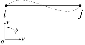
The beam element i j is analyzed in a local coordinate system, and its material parameters are known. The node displacement is shown in Figure 1.

FIGURE 1

FIGURE 1. Node displacement in local coordination.

The displacement component of the beam end can be expressed as follows:

$\delta ={\left[\begin{array}{cccccc}{u}_i& v_i& {\theta }_i& u_j& v_j& {\theta }_j\end{array}\right]}^{\text{T}}.(1)$

Thus, the stiffness matrix of the beam element in a local coordinate system can be obtained (Luo and Liu, 2016) as follows:

$k_e=\left[\begin{array}{cccccc}\frac{EA}{l}& 0& 0& -\frac{EA}{l}& 0& 0\\ 0& \frac{12EI}{l^3}& \frac{6EI}{l^2}& 0& -\frac{12EI}{l^3}& \frac{6EI}{l^2}\\ 0& \frac{6EI}{l^2}& \frac{4EI}{l}& 0& -\frac{6EI}{l^2}& \frac{2EI}{l}\\ -\frac{EA}{l}& 0& 0& \frac{EA}{l}& 0& 0\\ 0& -\frac{12EI}{l^3}& -\frac{6EI}{l^2}& 0& \frac{12EI}{l^3}& -\frac{6EI}{l^2}\\ 0& \frac{6EI}{l^2}& \frac{2EI}{l}& 0& -\frac{6EI}{l^2}& \frac{4EI}{l}\end{array}\right].(2)$

2.2 Element Stiffness Matrix in the Global Coordinate System

2.2.1 Forward Process

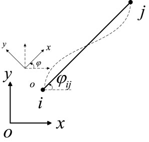
The beam element is placed in the global coordinate system (as shown in Figure 2 with the sequence of element connection from i point to j points). In order to obtain the element stiffness matrix of the beam element in the global system, we rotated the global coordinate system counterclockwise at an angle of φ_ij so that the axis x coincides with the axis of the beam element.

FIGURE 2

FIGURE 2. Global coordinate system rotation diagram (point i to point j).

According to the transformation relation between the global displacement and local displacement, the transformation matrix S_ij (YANG et al., 2019) can be obtained:

$S_{ij}=\left[\begin{array}{cccccc}\cos {\phi }_{ij}& \sin {\phi }_{ij}& 0& 0& 0& 0\\ -\sin {\phi }_{ij}& \cos {\phi }_{ij}& 0& 0& 0& 0\\ 0& 0& 1& 0& 0& 0\\ 0& 0& 0& \cos {\phi }_{ij}& \sin {\phi }_{ij}& 0\\ 0& 0& 0& -\sin {\phi }_{ij}& \cos {\phi }_{ij}& 0\\ 0& 0& 0& 0& 0& 1\end{array}\right].(3)$

Through the transformation matrix, the element stiffness matrix K_eij in the global coordinate system with the element connection relation from point i to point j can be obtained (Luo and Yan, 2015):

$K_{eij}=S_{ij}^T\cdot k_e\cdot S_{ij}.(4)$

2.2.2 Reverse Process

We selected the same beam element, as shown in Figure 3, with the element connection sequence from points j to i and rotated the global coordinate system counterclockwise at an angle of φ_ji so that axis x overlapped with the axis of the beam element.

FIGURE 3

FIGURE 3. Global coordinate system rotation diagram (point j to point i).

According to the coordinate correspondence φ_ji = 180^。+ φ_ij, the transformation matrix S_ji is as follows:

$S_{ji}=\left[\begin{array}{cccccc}\cos {\phi }_{ji}& \sin {\phi }_{ji}& 0& 0& 0& 0\\ -\sin {\phi }_{ji}& \cos {\phi }_{ji}& 0& 0& 0& 0\\ 0& 0& 1& 0& 0& 0\\ 0& 0& 0& \cos {\phi }_{ji}& \sin {\phi }_{ji}& 0\\ 0& 0& 0& -\sin {\phi }_{ji}& \cos {\phi }_{ji}& 0\\ 0& 0& 0& 0& 0& 1\end{array}\right].(5)$

Through the transformation matrix, the element stiffness matrix K_eji in the global coordinate system with the element connection relation from point j to point i can be obtained as follows:

$K_{eji}=S_{ji}^T\cdot k_e\cdot S_{ji}.(6)$

Comparing Eqs. 4–6, we can get

$K_{eij}\ne K_{eji}.(7)$

Therefore, for the same element, different connection sequences of elements will lead to inconsistency of the element stiffness matrix in the global coordinate system. The influence of such inconsistency on the global stiffness matrix of structure is worthy of further study.

3 Structural Global Matrix

For the element in Figure 2, the elastic strain energy e of the element can be expressed as follows: (Luo and Liu, 2016)

$e_{ij}=\frac{1}{2}{\delta }_{ij}^T{K}_{eij}{\delta }_{ij},(\mathrm{8a})$

$e_{ji}=\frac{1}{2}{\delta }_{ji}^T{K}_{eji}{\delta }_{ji}.(\mathrm{8b})$

The elastic strain energy E of the same element in the overall structure can be expressed as follows (Luo and Liu, 2016):

$E_{ij}=\frac{1}{2}{\text{Δ}}^T{K}_{gij}\text{Δ},(\mathrm{9a})$

$E_{ji}=\frac{1}{2}{\text{Δ}}^T{K}_{gji}\text{Δ}.(\mathrm{9b})$

According to the law of energy conservation, the elastic strain energy of the element remains unchanged no matter how the connection sequence and coordinate system are selected:

$e_{ij}=e_{ji},(\mathrm{10a})$

$E_{ij}=E_{ji},(\mathrm{10b})$

$e_{ij}=E_{ij},(\mathrm{10c})$

$e_{ji}=E_{ji}.(\mathrm{10d})$

Substituting Eqs. 9a,b into Eq. 10b, we obtain

$K_{gij}=K_{gji}.(11)$

Δ in Eqs. 9a,b is the displacement component of the overall frame structure. For the frame structure with n nodes, it can be expressed as a 3n F0B4 1 column vector.

$\text{Δ}={\left[\begin{array}{cccc}\begin{array}{cccc}\begin{array}{cccc}\begin{array}{cc}{u}_1& v_1\end{array}& {\theta }_1& \cdots & u_i\end{array}& v_i& \begin{array}{cc}{\theta }_i& \cdots \end{array}& u_j\end{array}& v_j& {\theta }_j& \cdots \end{array}\right]}^T.(12)$

The corresponding element displacement component is extracted from the displacement component of the overall frame structure, and a 6 F0B4 3n extraction matrix T (element subscript is the row and column) is established (Luo et al., 2019):

$T_{ij}=\left[\begin{array}{ccccccccccccc}\cdots & \text{0}& 1_{(\mathrm{1,3}i-2)}& \text{0}& \cdots & \cdots & \cdots & \cdots & \cdots & \cdots & \cdots & \cdots & \cdots \\ \cdots & \cdots & \text{0}& 1_{(\mathrm{2,3}i-1)}& \text{0}& \cdots & \cdots & \cdots & \cdots & \cdots & \cdots & \cdots & \cdots \\ \cdots & \cdots & \cdots & \text{0}& 1_{\left(\mathrm{3,3}i\right)}& \text{0}& \cdots & \cdots & \cdots & \cdots & \cdots & \cdots & \cdots \\ \cdots & \cdots & \cdots & \cdots & \cdots & \cdots & \cdots & \text{0}& 1_{(\mathrm{4,3}j-2)}& \text{0}& \cdots & \cdots & \cdots \\ \cdots & \cdots & \cdots & \cdots & \cdots & \cdots & \cdots & \cdots & \text{0}& 1_{(\mathrm{5,3}j-1)}& \text{0}& \cdots & \cdots \\ \cdots & \cdots & \cdots & \cdots & \cdots & \cdots & \cdots & \cdots & \cdots & \text{0}& 1_{\left(\mathrm{6,3}j\right)}& \text{0}& \cdots \end{array}\right],(\mathrm{13a})$

$T_{ji}=\left[\begin{array}{ccccccccccccc}\cdots & \cdots & \cdots & \cdots & \cdots & \cdots & \cdots & \text{0}& 1_{(\mathrm{4,3}j-2)}& \text{0}& \cdots & \cdots & \cdots \\ \cdots & \cdots & \cdots & \cdots & \cdots & \cdots & \cdots & \cdots & \text{0}& 1_{(\mathrm{5,3}j-1)}& \text{0}& \cdots & \cdots \\ \cdots & \cdots & \cdots & \cdots & \cdots & \cdots & \cdots & \cdots & \cdots & \text{0}& 1_{\left(\mathrm{6,3}j\right)}& \text{0}& \cdots \\ \cdots & \text{0}& 1_{(\mathrm{1,3}i-2)}& \text{0}& \cdots & \cdots & \cdots & \cdots & \cdots & \cdots & \cdots & \cdots & \cdots \\ \cdots & \cdots & \text{0}& 1_{(\mathrm{2,3}i-1)}& \text{0}& \cdots & \cdots & \cdots & \cdots & \cdots & \cdots & \cdots & \cdots \\ \cdots & \cdots & \cdots & \text{0}& 1_{\left(\mathrm{3,3}i\right)}& \text{0}& \cdots & \cdots & \cdots & \cdots & \cdots & \cdots & \cdots \end{array}\right].(\mathrm{13b})$

where T_ij represents the element displacement component extracted from the integral displacement component in the order that point i is connected to point j, and T_ji represents the element displacement component extracted from the integral displacement component in the order that point j is connected to point i.

From Eq. 1, Eq. 12, and Eqs. 13a,b, the process of extracting the element displacement component from the global displacement component can be expressed as follows:

${\delta }_{ij}=T_{ij}\text{Δ},(\mathrm{14a})$

${\delta }_{ji}=T_{ji}\text{Δ}.(\mathrm{14b})$

Substituting Equations 14a,b into Equations 8a,b we obtain

$e_{ij}=\frac{1}{2}{\text{Δ}}^T{T}_{ij}^T{K}_{eij}{T}_{ij}\text{Δ},(\mathrm{15a})$

$e_{ji}=\frac{1}{2}{\text{Δ}}^T{T}_{ji}^T{K}_{eji}{T}_{ji}\text{Δ}.(\mathrm{15b})$

Substituting Eq. 9a and Eq. 15a into Eq. 10c and at the same time substituting Eq. 9b and Eq. 15b into Eq. 10d, the conversion relationship of the element stiffness matrix in the global coordinate system can be obtained as follows:

$K_{gij}=T_{ij}^T{K}_{eij}{T}_{ij},(\mathrm{16a})$

$K_{gji}=T_{ji}^T{K}_{eji}{T}_{ji}.(\mathrm{16b})$

Therefore, by substituting Eqs. 4, 6 into Eq. 16a and Eq. 16b, we can obtain the following:

$K_{\mathrm{g}\mathrm{i}\mathrm{j}}=T_{\mathrm{i}\mathrm{j}}^T{S}_{\mathrm{i}\mathrm{j}}^T{k}_e{S}_{\mathrm{i}\mathrm{j}}{T}_{\mathrm{i}\mathrm{j}},(\mathrm{17a})$

$K_{\mathrm{g}\mathrm{i}\mathrm{j}}=T_{\mathrm{j}\mathrm{i}}^T{S}_{\mathrm{j}\mathrm{i}}^T{k}_{\mathrm{e}}{S}_{\mathrm{j}\mathrm{i}}{T}_{\mathrm{j}\mathrm{i}}.(\mathrm{17b})$

From Eq. 2, it is known that the element stiffness matrix k_e in the local coordinate system is unique. According to Eq. 7, in the process of transforming local coordinates into global coordinates, the stiffness matrix K_e of the element in the global coordinate system will change if different element connection relations are selected; however, in the process of the global stiffness assembly, the elements of K_e need to be extracted into the overall structure matrix according to Eqs. 16a,b, based on the corresponding relationship of the element node degrees of freedom. Therefore, the modeling of the element stiffness matrix is composed of two steps. The first step is to transform the element stiffness matrix in the local coordinate system into the global coordinate system, and the second step is to extract the element stiffness matrix elements in the global coordinate system into the global matrix.

It can be seen from Eq. 11 that the two stiffness matrices obtained by Eqs. 17a,b are the same, and changing the connection relation of elements does not affect the modeling results of the element stiffness matrix.

The elastic strain energy E_t of the given structure is expressed as follows:

$E_{\text{t}}=\frac{1}{2}{\text{Δ}}^T{K}_G\text{Δ}.(18)$

The elastic strain energy of the structure is the sum of the elastic strain energy of each element, namely,

$E_t={\displaystyle \sum E}.(19)$

Substituting Eq. 18 and Eqs. 9a,b into Eq. 19, we can obtain

$K_{Gij}={\displaystyle \sum K_{gij}},(\mathrm{20a})$

$K_{Gji}={\displaystyle \sum K_{gji}}.(\mathrm{20b})$

The comprehensive Eqs. 11–20 can be obtained as follows:

$K_{Gij}=K_{Gji}.(21)$

Finally, the boundary conditions of the structure are considered, and the rows and columns corresponding to the freedom of constraint in K_G are modified to obtain the global matrix K of the structure. Because the boundary conditions are the same, regardless of the selection of the node connection order, the result can be obtained as follows:

$K_{ij}=K_{ji}.(22)$

Therefore, for the same structure, different cell connection orders will not change the global matrix of the structure. This conclusion optimizes the process of overall structural analysis, especially the computer programming for frame structure, which can improve the logic of the program.

4 Example Analysis

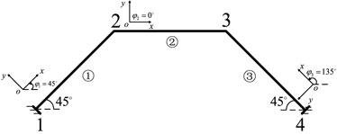
Taking the rigid frame structure shown in Figure 4 as an example, the section shapes and dimensions of element ①, element ②, and element ③ are equal. See Table 1 for various material properties of the beam element. The displacement and element internal force of the rigid frame structure under the action of external force are calculated.

FIGURE 4

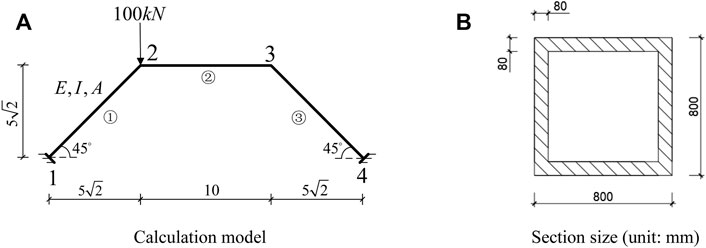
FIGURE 4. Calculation model and the section size of the rigid frame. (A) Calculation model. (B) Section size (unit: mm).

TABLE 1

TABLE 1. Table of the structural unit material property.

4.1 Forward Process

The global matrix of the structure is calculated, according to the node coding shown in Figure 5.

FIGURE 5

FIGURE 5. Node coding (point i to point j).

In the first step, the stiffness matrix k_e is found to be the same for all three elements in the figure in the local coordinate system, according to Eq. 2.

In the second step, the coordinate conversion matrix S of each element is found. For element ①, the tilt angle is 45^。. Element ② has no inclination, that is, the global coordinate system coincides with the local coordinate system. For element ③, the tilt angle is 135^。. By substituting the inclination angle of each element into Eq. 3, the conversion matrices S_ij¹, S_ij², and S_ij³ corresponding to element ①, element ②, and element ③ can be obtained.

In the third step, the stiffness matrix K_e of each element in the global coordinate system is obtained. By substituting the transformation matrices S_ij¹, S_ij², and S_ij³ of each element into Eq. 4, the stiffness matrices K_eij¹, K_eij², and K_eij³ corresponding to element ①, element ②, and element ③ in the global coordinate system can be obtained, respectively.

$K_{eij}^1=\left[\begin{array}{cccccc}2.4402& 2.3898& -0.1782& -2.4402& -2.3898& -0.1782\\ 2.3898& 2.4402& 0.1782& -2.3898& -2.4402& 0.1782\\ -0.1782& 0.1782& 1.6800& 0.1782& -0.1782& 0.8400\\ -2.4402& -2.3898& 0.1782& 2.4402& 2.3898& 0.1782\\ -2.3898& -2.4402& -0.1782& 2.3898& 2.4402& -0.1782\\ -0.1782& 0.1782& 0.8400& 0.1782& -0.1782& 1.6800\end{array}\right]\times {10}^6,(23)$

$k_{eij}^2=\left[\begin{array}{cccccc}4.8300& 0& 0& -4.8300& 0& 0\\ 0& 0.0504& 0.2520& 0& -0.0504& 0.2520\\ 0& 0.2520& 1.6800& 0& -0.2520& 0.8400\\ -4.8300& 0& 0& 4.8300& 0& 0\\ 0& -0.0504& -0.2520& 0& 0.0504& -0.2520\\ 0& 0.2520& 0.8400& 0& -0.2520& 1.6800\end{array}\right]\times {10}^6,(24)$

$K_{eij}^3=\left[\begin{array}{cccccc}2.4402& -2.3898& -0.1782& -2.4402& 2.3898& -0.1782\\ -2.3898& 2.4402& -0.1782& 2.3898& -2.4402& -0.1782\\ -0.1782& -0.1782& 1.6800& 0.1782& 0.1782& 0.8400\\ -2.4402& 2.3898& 0.1782& 2.4402& -2.3898& 0.1782\\ 2.3898& -2.4402& 0.1782& -2.3898& 2.4402& 0.1782\\ -0.1782& -0.1782& 0.8400& 0.1782& 0.1782& 1.6800\end{array}\right]\times {10}^6.(25)$

In the fourth step, the extraction matrix T of the stiffness matrix of each element is determined, according to the location of the element displacement component in the global displacement component. According to Eq. 13a, the extraction matrices corresponding to element ①, element ②, and element ③ are T_ij¹, T_ij², and T_ij³, respectively.

In the fifth step, K_g is obtained according to the transformation relation of the element stiffness matrix in the global coordinate system. Substituting K_eij¹ and T_ij¹ into Eq. 16a, we can obtain K_gij¹ of element ①; substituting K_eij² and T_ij² into Eq. 16a, we can obtain K_gij² of element ②; and substituting K_eij³ and T_ij³ into Eq. 16a, we can obtain K_gij³ of element ③.

In the sixth step, it can be seen from Eq. 20a that K_gij of the three elements is accumulated to obtain the 12th order structural global matrix K_Gij.

In the seventh step, it can be seen from Figure 5 that node 1 and node 4 have fixed end constraints, so the node displacement and rotation angle of these two points are 0. Therefore, the row and column corresponding to the displacement component of node 1 and node 4 in K_Gij are deleted, and the global matrix K_ij of the rigid frame structure in Figure 5 is obtained as follows:

$K_{ij}=\left[\begin{array}{cccccc}7.2702& 2.3898& 0.1782& -4.8300& 0& 0\\ 2.3898& 2.4906& 0.0738& 0& -0.0504& 0.2520\\ 0.1782& 0.0738& 3.3600& 0& -0.2520& 0.8400\\ -4.8300& 0& 0& 7.2702& -2.3898& 0.1782\\ 0& -0.0504& -0.2520& -2.3898& 2.4906& -0.0738\\ 0& 0.2520& 0.8400& 0.1782& -0.0748& 3.3600\end{array}\right]\times {10}^6.(26)$

4.2 Reverse Process

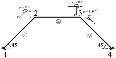
The global matrix of the structure is calculated according to the node coding shown in Figure 6.

FIGURE 6

FIGURE 6. Node coding (point j to point i).

In the first step, the stiffness matrix k_e of the three elements in the local coordinate system is found according to Eq. 2.

In the second step, the coordinate conversion matrix S of each element is found. For element ①, the tilt angle is 225°. For element ②, the tilt angle is 180°; for element ③, the tilt angle is 315°. By substituting the inclination angle of each element into Eq. 5, the conversion matrices S_ji¹, S_ji², and S_ji³ corresponding to element ①, element ②, and element ③ can be obtained.

In the third step, the stiffness matrix K_e of each element in the global coordinate system is obtained. By substituting the transformation matrices S_ji¹, S_ji², and S_ji³ of each element into Eq. 6, the stiffness matrices K_eji¹, K_eji², and K_eji³ corresponding to element ①, element ②, and element ③ in the global coordinate system can be obtained, respectively.

$K_{eji}^1=\left[\begin{array}{cccccc}2.4402& 2.3898& 0.1782& -2.4402& -2.3898& 0.1782\\ 2.3898& 2.4402& -0.1782& -2.3898& -2.4402& -0.1782\\ 0.1782& -0.1782& 1.6800& -0.1782& 0.1782& 0.8400\\ -2.4402& -2.3898& -0.1782& 2.4402& 2.3898& -0.1782\\ -2.3898& -2.4402& 0.1782& 2.3898& 2.4402& 0.1782\\ 0.1782& -0.1782& 0.8400& -0.1782& 0.1782& 1.6800\end{array}\right]\times {10}^6,(27)$

$K_{eji}^2=\left[\begin{array}{cccccc}4.8300& 0& 0& -4.8300& 0& 0\\ 0& 0.0504& -0.2520& 0& -0.0504& 0.2520\\ 0& -0.2520& 1.6800& 0& 0.2520& 0.8400\\ -4.8300& 0& 0& 4.8300& 0& 0\\ 0& -0.0504& 0.2520& 0& 0.0504& 0.2520\\ 0& -0.2520& 0.8400& 0& 0.2520& 1.6800\end{array}\right]\times {10}^6,(28)$

$K_{eji}^3=\left[\begin{array}{cccccc}2.4402& -2.3898& 0.1782& -2.4402& 2.3898& 0.1782\\ -2.3898& 2.4402& 0.1782& 2.3898& -2.4402& 0.1782\\ 0.1782& 0.1782& 1.6800& -0.1782& -0.1782& 0.8400\\ -2.4402& 2.3898& -0.1782& 2.4402& -2.3898& -0.1782\\ 2.3898& -2.4402& -0.1782& -2.3898& 2.4402& -0.1782\\ 0.1782& 0.1782& 0.8400& -0.1782& -0.1782& 1.6800\end{array}\right]\times {10}^6.(29)$

In the fourth step, the extraction matrix T of the stiffness matrix of each element is determined, according to the location of the element displacement component in the global displacement component. According to Eq. 13b, the extraction matrices corresponding to element ①, element ②, and element ③ are T_ji¹, T_ji², and T_ji³, respectively.

In the fifth step, K_g is obtained according to the transformation relation of the element stiffness matrix in the global coordinate system. Substituting K_eji¹ and T_ji¹ into Eq. 16b, we can obtain K_gji¹ of element ①; substituting K_eji² and T_ji² into Eq. 16b, we can obtain K_gji² of element ②; and substituting K_eji³ and T_ji³ into Eq. 16b, we can obtain K_gji³ of element ③.

In the sixth step, it can be seen from Eq. 20b that K_gji of the three units is accumulated to obtain the 12-order structural global matrix K_Gji.

In the seventh step, it can be seen from Figure 6 that node 1 and node 4 are constrained by fixed ends, so the node displacement and rotation angle of these two points are 0. Therefore, the row and column corresponding to the displacement component of node 1 and node 4 in K_Gji are deleted, and the global matrix K_ji of the rigid frame structure in Figure 6 is obtained as follows:

$K_{ji}=\left[\begin{array}{cccccc}7.2702& 2.3898& 0.1782& -4.8300& 0& 0\\ 2.3898& 2.4906& 0.0738& 0& -0.0504& 0.2520\\ 0.1782& 0.0738& 3.3600& 0& -0.2520& 0.8400\\ -4.8300& 0& 0& 7.2702& -2.3898& 0.1782\\ 0& -0.0504& -0.2520& -2.3898& 2.4906& -0.0738\\ 0& 0.2520& 0.8400& 0.1782& -0.0748& 3.3600\end{array}\right]\times {10}^6.(30)$

Through the example, we can find K_eij≠K_eji and K_ij = K_ji and verify the conclusion of Eqs. 7, 22.

4.3 Displacement and Bearing Reaction

In the first step, the external load vector F is established. According to Figure 4, a vertical external force of 100 KN is applied at node 2, which is expressed as a column vector given as follows:

$F={\left[\begin{array}{cc}\begin{array}{ccc}\begin{array}{ccc}\begin{array}{c}\begin{array}{c}0\end{array}\end{array}& -100& 0\end{array}& 0& 0\end{array}& 0\end{array}\right]}^T.(31)$

In the second step, the structural stiffness equation is established as follows:

$KU=F.(32)$

The displacement vector U can be obtained by transforming Eq. 32:

$U=K^{-1}F.(33)$

In the third step, the displacement vector U can be obtained by substituting Eqs. 26, 31 into Eq. 33:

$U=\left[\begin{array}{c}2.554m\\ -2.819m\\ 0.071rad\\ 2.452\\ 2.307m\\ 0.114rad\end{array}\right]\times {10}^{-4}.(34)$

The first three lines of Eq. 34 represent the displacement and rotation angle of node 2, and the last three lines represent the displacement and rotation angle of node 3.

The fourth step determined the stiffness equation of the complete structure, which is given as follows:

$K_G\text{Δ}=R.(35)$

where R is the load array of four nodes in the structure; it is expressed as follows:

$R={\left[\begin{array}{cccccccccccc}{R}_{1x}& R_{1y}& R_{1\theta }& R_{2x}& R_{2y}& R_{2\theta }& R_{3x}& R_{3y}& R_{3\theta }& R_{4x}& R_{4y}& R_{4\theta }\end{array}\right]}^T.(36)$

Eq. 36 can be transformed into a column vector of 4ⅹ1.

$R={\left[\begin{array}{cccc}{R}_1& R_2& R_3& R_4\end{array}\right]}^T.(37)$

According to Eq. 12, Δ is the displacement array of four nodes in the structure, which can be transformed into the column vector of 4ⅹ1.

$\text{Δ}={\left[\begin{array}{cccc}{\text{Δ}}_1& {\text{Δ}}_2& {\text{Δ}}_3& {\text{Δ}}_4\end{array}\right]}^T.(38)$

Because there is a fixed end constraint between node 1 and node 4, the displacement and rotation angle of node 1 and node 4 are 0, so

$\text{Δ}={\left[\begin{array}{cccc}0& {\text{Δ}}_2& {\text{Δ}}_3& 0\end{array}\right]}^T.(39)$

In the fifth step, K_e is divided into a stiffness sub block array in the order of connecting point i to point j and loaded into the global matrix K_G (the process of point j connecting to point i is similar, and the final K_G result is the same, so it will not be described here)

Element ① is split from node 1 to node 2:

$K_e^1=\left[\begin{array}{cc}{K}_{e11}^1& K_{e12}^1\\ K_{e21}^1& K_{e22}^1\end{array}\right].(40)$

Element ② is split from node 2 to node 3:

$K_e^2=\left[\begin{array}{cc}{K}_{e22}^2& K_{e23}^2\\ K_{e32}^2& K_{e33}^2\end{array}\right].(41)$

Element ③ is split from node 4 to node 3:

$K_e^3=\left[\begin{array}{cc}{K}_{e44}^3& K_{e43}^3\\ K_{e34}^3& K_{e33}^3\end{array}\right].(42)$

The global stiffness matrix K_G can be obtained by combining the element stiffness matrix derived from Eqs. 40–42, and the global stiffness matrix K_G is expressed as follows:

$K_G=\left[\begin{array}{cccc}{K}_{e11}^1& K_{e12}^1& 0& 0\\ K_{e21}^1& K_{e22}^1+K_{e22}^2& K_{e23}^2& 0\\ 0& K_{e32}^2& K_{e33}^2+K_{e33}^3& K_{e34}^3\\ 0& 0& K_{e43}^3& K_{e44}^3\end{array}\right].(43)$

In the sixth step, the support reaction of constrained nodes is calculated.

Substituting Eqs. 37, 39 and 43 into Eq. 35, we can obtain the following:

$K_{e12}^1\cdot {\mathrm{\Delta }}_2=R_1,(44)$

$K_{e43}^3\cdot {\mathrm{\Delta }}_3=R_4.(45)$

where the significance of the stiffness sub-block K_e12¹ is the force generated by node 1 when node 2 has element displacement in the global coordinate system. According to Eq. 23, the stiffness sub-block K_e12¹ is

$K_{e12}^1=\left[\begin{array}{ccc}-2.4402& -2.3898& -0.1782\\ -2.3898& -2.4402& 0.1782\\ 0.1782& -0.1782& 0.8400\end{array}\right]\times {10}^6.(46)$

The significance of the stiffness sub-block K_e43³ is the force generated at node 4 when node 3 has unit displacement in the global coordinate system. According to Eq. 25, the stiffness sub-block K_e43³ is as follows:

$K_{e43}^3=\left[\begin{array}{ccc}-2.4402& 2.3898& -0.1782\\ 2.3898& -2.4402& -0.1782\\ 0.1782& 0.1782& 0.8400\end{array}\right]\times {10}^6.(47)$

According to Eq. 34, it can be known as

${\text{Δ}}_2={\left[\begin{array}{ccc}2.554& -2.819& 0.071\end{array}\right]}^T\times {10}^{-4},(48)$

${\text{Δ}}_3={\left[\begin{array}{ccc}2.452& 2.307& 0.114\end{array}\right]}^T\times {10}^{-4}.(49)$

Substituting Eqs. 46, 48 into Eq. 44, we can obtain

$R_1={\left[\begin{array}{ccc}49\text{.}1923\text{kN}& 78\text{.}8027\text{kN}& 101\text{.}7109\text{kN}\cdot \text{m}\end{array}\right]}^T.(50)$

Substituting Eqs. 47, 49 into Eq. 45, we can obtain

$R_4={\left[\begin{array}{ccc}-49\text{.}0417\text{kN}& 20\text{.}9933\text{kN}& 94\text{.}3814\text{kN}\cdot \text{m}\end{array}\right]}^T.(51)$

Because R₁ contains the known external load array F₁ and the reaction force f₁ on the supporting node,

$f_1=R_1-F_1.(52)$

The same can be given as follows:

$f_4=R_4-F_4.(53)$

There is no external load on node 1 and node 4, so

$F_1={\left[\begin{array}{ccc}0& 0& 0\end{array}\right]}^T,(54)$

$F_4={\left[\begin{array}{ccc}0& 0& 0\end{array}\right]}^T.(55)$

By substituting Eqs. 50, 54 into Eq. 52, the supporting reaction force at node 1 can be obtained as follows:

$f_1={\left[\begin{array}{ccc}49\text{.}1923\text{kN}& 78\text{.}8027\text{kN}& 101\text{.}7109\text{kN}\cdot \text{m}\end{array}\right]}^T.(56)$

By substituting Eqs. 52, 55 into Eq. 53, the supporting reaction force at node 4 can be obtained as follows:

$f_4={\left[\begin{array}{ccc}-49\text{.}0417\text{kN}& 20\text{.}9933\text{kN}& 94\text{.}3814\text{kN}\cdot \text{m}\end{array}\right]}^T.(57)$

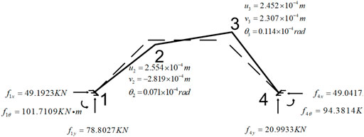
The drawing of deformation diagram of rigid frame structure is shown in Figure 7 (solid line after deformation and dotted line before deformation).

FIGURE 7

FIGURE 7. Frame structure deformation diagram.

4.4 Structural Dynamic Analysis Based on the State Space Model

We continued taking the rigid frame structure shown in Figure 4 as an example to analyze the dynamic response of the rigid frame under different working conditions, the specific working conditions are shown in Table 2.

TABLE 2

TABLE 2. Calculation cases.

The working conditions are as follows: by comparing cases 1 to 4 to study the dynamic response of rigid frame structures with different damping ratios when the harmonic excitation (frequency: 11 Hz) is equal; by comparing cases 5 to 8 to study the dynamic response of rigid frame structures with different damping ratios when harmonic excitation (frequency is the first-order frequency of the structure) causes structural resonance; and by comparing cases 1 to 4 with cases 5 to 8 to study the dynamic response of the structure under different excitations when the damping ratio is the same; cases 9 to 12 are used to investigate whether the dynamic response of the structure under the excitation of EL Centro seismic waves conforms to the laws of the dynamic response of the structure discussed in cases 1 to 8.

4.4.1 Dynamic Response Analysis Process of Example

In the first step, the global mass matrix is established in the global coordinate system M_G.

The element mass matrix in the local coordinate system is (Ding and Chen, 2006)

$m_e=\frac{\rho Al}{420}\left[\begin{array}{cccccc}140& 0& 0& 70& 0& 0\\ 0& 156& 22l& 0& 54& -13l\\ 0& 22l& 4l^2& 0& 13l& -3l^2\\ 70& 0& 0& 140& 0& 0\\ 0& 54& 13l& 0& 156& -22l\\ 0& -13l& -3l^2& 0& -22l& 4l^2\end{array}\right].(58)$

Similarly, through the transformation matrix S_ij of Eq. 5, the element mass matrix m_e in the local coordinate system can be transformed into the element mass matrix M_eij in the global coordinate system.

$M_{eij}=S_{ij}^T•m_e•S_{ij}.(59)$

The matrix T_ij is extracted by Eq. 13a, and each element in M_e is extracted into the global structure matrix.

$M_{gij}=T_{ij}^T•S_{ij}^T•m_e•S_{ij}•T_{ij}^T.(60)$

The global mass matrix M_Gij of the structure under the global coordinate system is obtained by accumulation.

$M_{Gij}={\displaystyle \sum M_{gij}}.(61)$

According to the parameters in Figure 4 and Table 1, the global mass matrix M_G of the structure in the global coordinate system is calculated.

In the second step, the treatment of boundary conditions of the finite element method is carried out (mark 0 to set 1) (Reddy, 2019).

As shown in Figure 4, because node 1 and node 4 are fixed ends, each fixed end has three constraints. Therefore, the boundary conditions of the global mass matrix M_G and the global stiffness matrix K_G of the structure in the global coordinate system are processed, respectively (mark 0 to set 1) the global mass matrix M_Z and global stiffness matrix K_Z of the structure in the processed global coordinate system are obtained.

In the third step, the damping matrix is established.

In general, Rayleigh damping can be expressed as follows (Cruz and Miranda, 2017):

$\left[C_z\right]=a_0\left[M_z\right]+a_1\left[K_z\right],(62)$

where a₀ and a₁ are two scaling coefficients.

$a_0=\frac{2\zeta {\omega }_1{\omega }_2}{{\omega }_1+{\omega }_2},a_1=\frac{2\zeta }{{\omega }_1+{\omega }_2},(63)$

where ω₁ and ω₂ represent the first-order frequency and the second-order frequency, respectively, and ζ represents the structural damping ratio. For convenience, the first two modal damping values of the structure analyzed in this study are the same.

The damping ratios are 0.01, 0.015, 0.02, and 0.025, respectively, and brought into Eq. 62 together with M_Z, K_Z, and Eq. 63; the damping matrices C_z0.01, C_z0.015, C_z0.02, and C_z0.025 of the steel frame structure are obtained, respectively.

In the fourth step, based on the state space model, the dynamic analysis of the rigid frame structure is carried out.

The discrete-time state space model of the system can be expressed as follows: (Moonen et al., 1989; Swindlehust et al., 1995; Bernal et al., 2015)

$\mathit{X}\left[k+1\right]=\mathit{A}\mathit{X}\left[k\right]+\mathit{B}\mathit{U}\left[k\right],(64)$

$\mathit{Y}\left[k\right]={\mathit{C}}_1\mathit{X}\left[k\right]+\mathit{D}\mathit{U}\left[k\right].(65)$

Among them,

$\mathit{A}=e^{A_c\text{Δ}t},(66)$

$\mathit{B=}{\displaystyle {\int }_{\mathit{0}}^{\text{Δ}\mathit{t}}{\mathrm{e}}^{A_{\mathit{c}}\tau }{\mathit{B}}_{\mathbf{c}}d\tau ={\mathit{A}}_{\mathbf{c}}^{-1}\left(\mathit{A}-1\right){\mathit{B}}_{\mathbf{c}}},(67)$

${\mathit{C}}_1={\mathit{C}}_{\mathbf{c}}=\left[\begin{array}{cc}{\mathit{C}}_{\mathbf{d}}-{\mathit{C}}_{\mathbf{a}}{\mathit{M}}^{-1}\mathit{K}& {\mathit{C}}_{\mathbf{v}}-{\mathit{C}}_{\mathrm{a}}{\mathit{M}}^{-1}\mathit{C}\end{array}\right],(68)$

$\mathit{D}={\mathit{D}}_{\mathbf{c}}={\mathit{C}}_{\mathbf{a}}{\mathit{M}}^{-1}.(69)$

A is the state matrix of the discrete-time system, B is the input matrix of the discrete-time system, and C₁ and D are the observation matrices of the state and input of the discrete-time system, respectively. Δt is the sampling period, C_a, C_v, and C_d are the acceleration output matrix, velocity output matrix, and displacement output matrix, respectively, A_c is the state matrix of the structural continuous time system, and B_c is the input matrix of the structural continuous time system.

${\mathit{A}}_{\mathrm{c}}=\left[\begin{array}{cc}\mathbf{0}& I\\ -{\mathit{M}}^{-1}\mathit{K}& -{\mathit{M}}^{-1}\mathit{C}\end{array}\right],{\mathit{B}}_{\mathrm{c}}=\left[\begin{array}{c}\mathbf{0}\\ {\mathit{M}}^{-1}\end{array}\right],(70)$

I is the identity matrix, C is the damping matrix, M and K are the global mass matrix and global stiffness matrix after finite element boundary condition treatment, respectively.

4.4.2 Dynamic Response Analysis of the Rigid Frame Structure

4.4.2.1 Dynamic Response of the Rigid Frame Structure Under Harmonic Excitation

The discrete-time state space model is used to describe the system. The sampling frequency is set as Fs = 200Hz, the sampling interval as 1/Fs, and the number of generated samples as N = 1,000 to sample the output displacement, output speed, and output acceleration, respectively.

(1) Dynamic response of the rigid frame structure under the harmonic excitation with a frequency of 11 Hz.

When the harmonic excitation with a frequency of 11 Hz is adopted, the output response of the system under different damping ratios is recorded from the initial time, as shown in Figure 8A–D.

(2) Dynamic responses of the rigid frame structure under the harmonic excitation with a frequency of 13.3592 Hz

FIGURE 8

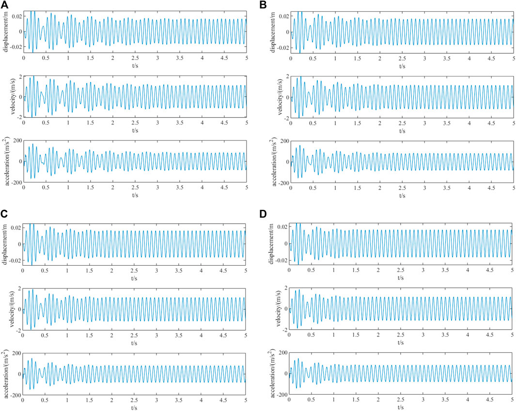
FIGURE 8. (A) Time history curve of the output response under harmonic excitation (f = 11 Hz and ζ = 0.01). (B) Time history curve of the output response under harmonic excitation (f = 11 Hz and ζ = 0.015), (C) Time history curve of the output response under harmonic excitation (f = 11 Hz and ζ = 0.02). (D) Time history curve of the output response under harmonic excitation (f = 11 Hz and ζ = 0.025).

Because the first-order natural frequency of the structure is 13.3592 Hz, the structure resonates when the frequency of harmonic excitation is 13.3592 Hz. The output response of the system under different damping ratios is recorded from the initial time, as shown in Figures 9A–D.

FIGURE 9

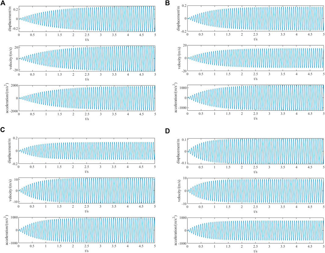
FIGURE 9. (A) Time history curve of the output response under harmonic excitation (f = 13.3592 Hz and ζ = 0.01). (B) Time history curve of the output response under harmonic excitation (f = 13.3592 Hz and ζ = 0.015). (C) Time history curve of the output response under harmonic excitation (f = 13.3592 Hz and ζ = 0.02). (D) Time history curve of the output response under harmonic excitation (f = 13.3592 Hz and ζ = 0.025).

4.4.2.2 Dynamic Response of the Rigid Frame Structure Excited by an El Centro Seismic Wave

The discrete-time state space model is used to describe the system. The drive of the system is the seismic wave input. The seismic wave adopts 500gal El Centro wave, the sampling period is 0.02s, and the number of generated samples is N = 1,500.

When El Centro seismic wave excitation is adopted, the output response of the system under different damping ratios is recorded from the initial time, as shown in Figures 10A–D.

FIGURE 10

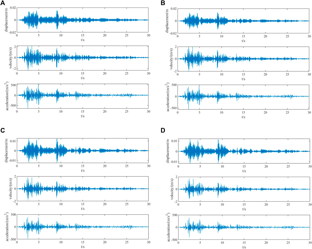
FIGURE 10. (A) Time history curve of the output response under El Centro seismic wave excitation (ζ = 0.01). (B) Time history curve of the output response under El Centro seismic wave excitation (ζ = 0.015). (C) Time history curve of the output response under El Centro seismic wave excitation (ζ = 0.02).(D) Time history curve of the output response under El Centro seismic wave excitation (ζ = 0.025)

The peak values of displacement, velocity, and acceleration of each case of the structure are extracted, respectively. The specific data are shown in the table as follows.

In order to more clearly show the relationship between the structural damping ratio and displacement, and velocity and acceleration under different external excitation, we draw the data in Table 3 into a broken line diagram, as shown in Figures 11A–C.

TABLE 3

TABLE 3. Peak values of displacement, velocity, and acceleration of structures under different cases.

FIGURE 11

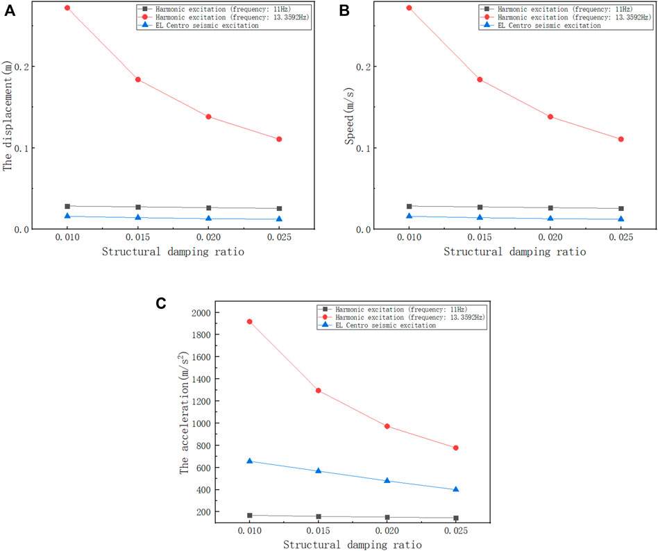
FIGURE 11. (A) Relationship between the damping ratio and displacement. (B) Relationship between the damping ratio and velocity. (C) Relationship between the damping ratio and acceleration.

Combined with Table 3 and Figure 11, it can be seen that in cases 1 to 4, under the harmonic excitation with a frequency of 11Hz, when the damping ratio is 0.01, the displacement, velocity, and acceleration of the rigid frame structure reach the maximum, which are 0.0283m, 2.0936 m/s, and 168.1733 m/s²⁰, respectively; when the damping ratio is 0.025, the displacement, velocity, and acceleration of the rigid frame structure reach the minimum values, which are 0.0255m, 1.8786 m/s, and 144.6427 m/s², respectively. In the working conditions 5 to 8, under the harmonic excitation with a frequency of 13.3592Hz, when the damping ratio is 0.01, the displacement, velocity, and acceleration of the rigid frame structure reach the maximum, which are 0.2724m, 22.8122 m/s, and 1917m/s², respectively; when the damping ratio is 0.025, the displacement, velocity, and acceleration of the rigid frame structure reach the minimum values of 0.1107m, 9.2911 m/s, and 777.6984 m/s², respectively. It can be seen that under the same excitation, with the increase in the damping ratio, the displacement, velocity, and acceleration of the rigid frame structure gradually decrease, and the structure gradually tends to be stable; moreover, in the structural dynamic analysis, the value of the damping ratio will affect the accuracy of structural dynamic response analysis.

Through the comparative analysis of cases 1 to 4 and cases 5 to 8, it can be seen that in cases 5 to 8, when the excitation frequency is equal to the natural frequency of the rigid frame structure, the structure resonates. At the same damping ratio, the acceleration of the structure is much greater than the corresponding acceleration in cases 1 to 4.

In cases 9 to 12, under the excitation of the El Centro seismic wave, with the increase in the damping ratio, the displacement, velocity, and acceleration of the rigid frame structure gradually decrease, and the structure tends to be stable; moreover, the dynamic response of the rigid frame structure caused by the El Centro seismic wave is less than that of structure resonance. It conforms to the law obtained from the comparative analysis of cases 1 to 8.

5 Conclusion

In the stress analysis of steel structures, whether static analysis or dynamic analysis, it is necessary to establish the structural stiffness matrix first. In the process of establishing the structural stiffness matrix, there are usually different coding sequences of nodes for the same element. In this study, the influence of the change in the connection order of element nodes on the global matrix of the structure is discussed, and the mechanical analysis of steel structures is carried out, and the following conclusions are obtained through theoretical deduction and calculation example analysis:

(1) For the same elements, different nodal connection orders will lead to different element stiffness matrices in the global coordinate system due to the change in the coordinate axis direction.

(2) Although the element stiffness matrices under the established global coordinate system are different, in the process of integrating the global stiffness matrix, the elements of the global stiffness matrix obtained by reordering the corresponding relationship between the node code and the matrix elements are the same. Therefore, there is no difference in the global stiffness matrix of the structure established by changing the node connection relationship, which will not affect the stress analysis of the steel structure. This conclusion provides a reliable theoretical basis for the situation that the order of node connections need not be consistent in the finite element modeling of steel structures and is of reference value for the finite element modeling of steel structures.

(3) When analyzing the dynamic response of rigid frame structures, the dynamic response structure of the structure analyzed by different external excitation processes is different; when the frequency of external excitation is equal to the natural frequency of the structure, the dynamic response value of the structure reaches the peak and the structure resonates.

(4) Although the change in the damping ratio is small, the peak acceleration of the structure changes obviously. Therefore, the value of the damping ratio will affect the accuracy of the results of structural dynamic analysis.

Data Availability Statement

The original contributions presented in the study are included in the article/supplementary materials; further inquiries can be directed to the corresponding author.

Author Contributions

SL is responsible for pushing the theoretical part; DS and K are responsible for example design and analysis, and writing articles; RF and WW are responsible for further revision and improvement of the manuscript.

Conflict of Interest

Author RF is employed by Tongchuang Engineering Design Company.

The remaining authors declare that the research was conducted in the absence of any commercial or financial relationships that could be construed as a potential conflict of interest.

Publisher’s Note

All claims expressed in this article are solely those of the authors and do not necessarily represent those of their affiliated organizations, or those of the publisher, the editors, and the reviewers. Any product that may be evaluated in this article, or claim that may be made by its manufacturer, is not guaranteed or endorsed by the publisher.

References

Azim, M. R., and Gül, M. (2021). Data-driven Damage Identification Technique for Steel Truss Railroad Bridges Utilizing Principal Component Analysis of Strain Response. Struct. Infrastructure Eng., 17(8): 1019–1035.doi:10.1080/15732479.2020.1785512

CrossRef Full Text | Google Scholar

Bathe, K. J. (1996). Finite Element Procedures. Englewood Cliffs, NJ: Prentice-Hall

Google Scholar

Bernal, D., Döhler, M., Kojidi, S. M., Kwan, K., and Liu, Y. (2015). First Mode Damping Ratios for Buildings. Earthq. Spectra 31 (1), 367–381. doi:10.1193/101812eqs311m

CrossRef Full Text | Google Scholar

Cruz, C., and Miranda, E. (2017). Evaluation of the Rayleigh Damping Model for Buildings. Eng. Struct. 138, 324–336. doi:10.1016/j.engstruct.2017.02.001

CrossRef Full Text | Google Scholar

Ding, K., and Chen, Y. (2006). Finite Element Method. Beijing: Peking University Press. 121.

Google Scholar

Doebling, S. W., Peterson, L. D., and Alvin, K. F. (1998). Experimental Determination of Local Structural Stiffness by Disassembly of Measured Flexibility Matrices. J. Vib. Acoust. ASME 120, 949–957. doi:10.1115/1.2893925

CrossRef Full Text | Google Scholar

Feng, X. (2018). An Investigation on Optimal Initial Self-Stress Design of Tensegrity Grid Structures. Int. J. Steel Struct. 18 (3), 960–975. doi:10.1007/s13296-018-0040-z

CrossRef Full Text | Google Scholar

Feng, X., Miah, M. S., Ou, Y., and Ou, Y. W. (2018). Dynamic Behavior and Vibration Mitigation of a Spatial Tensegrity Beam. Eng. Struct. 171, 1007–1016. doi:10.1016/j.engstruct.2018.01.045

CrossRef Full Text | Google Scholar

Iu, C. K., and Bradford, M. A. (2010). Second-order Elastic Finite Element Analysis of Steel Structures Using a Single Element Per Member. Eng. Struct. 32 (9), 2606–2616. doi:10.1016/j.engstruct.2010.04.033

CrossRef Full Text | Google Scholar

Kamiński, M., and Supeł, K. (2016). Elastic Critical Moment for Bisymmetric Steel Profiles and its Sensitivity by the Finite Difference Method. Int. J. Appl. Mech. Eng., 21(1), 37–59. doi:10.1515/ijame-2016-0003

CrossRef Full Text | Google Scholar

Katebi, L., Tehranizadeh, M., and Mohammadgholibeyki, N. (2018). A Generalized Flexibility Matrix-Based Model Updating Method for Damage Detection of Plane Truss and Frame Structures. J. Civ. Struct. Health Monit. 8 (2), 301–314. doi:10.1007/s13349-018-0276-5

CrossRef Full Text | Google Scholar

Li, G., Luo, S., and Li, Z. (2020). Damage Diagnosis of Modal Flexibility Based on Degree of Freedom Reduction. Chin. Q. Mech., 41(3): 554–561. doi:10.21656/1000-0887.410138

CrossRef Full Text | Google Scholar

Luo, S., and Liu, W. (2016). Coordinate Transformation Method of Finite Element Model for Frame Structures. J. Shaoxing Univ. Nat. Sci., 36(02): 17–23. doi:10.16169/j.issn.1008-293x.k.2016.08.04

CrossRef Full Text | Google Scholar

Luo, S., Shen, K., Shen, J., and Li, J. (2019). Element Stiffness Matrix Decomposition Method for Frame Structure Damage Identification. J. Jiamusi Univ. Nat. Sci. Ed., 06:858–860+1009.

Google Scholar

Luo, S., and Yan, Q. (2015). Coordinate Transformation Method of Finite Element Model for Truss Structures. Sichuan Build. Sci., 41(3):10–13. doi:10.3969/j.issn.1008-1933.2015.03.003

CrossRef Full Text | Google Scholar

Luo, S., and Yang, Q. (2021). Natural Frequency Measurement of Steel Components by the Sound Signal. J. Low Freq. Noise, Vib. Act. Control 40 (2), 993–1004. doi:10.1177/1461348419860712

CrossRef Full Text | Google Scholar

Luo, S., Zhu, J., Liang, C., and Liu, W. (2018). Assembling Global Stiffness Matrix for Finite Element Model. J. Shenzhen Univ. Sci. Eng. 35 (5), 467–472. doi:10.3724/sp.j.1249.2018.05467

CrossRef Full Text | Google Scholar

Mignolet, M. P., Soize, C., and Avalos, J. (2013). Nonparametric Stochastic Modeling of Structures with Uncertain Boundary Conditions/Coupling Between Substructures. AIAA J. 51 (6), 1296–1308. doi:10.2514/1.j051555

CrossRef Full Text | Google Scholar

Moonen, M., De Moor, B., Vandenberghe, L., and Vandewalle, J. (1989). On- and Off-Line Identification of Linear State-Space Models. Int. J. Control 49 (1), 219–232. doi:10.1080/00207178908559631

CrossRef Full Text | Google Scholar

Pindera, M.-J. (1991). Local/global Stiffness Matrix Formulation for Composite Materials and Structures. Compos. Eng. 1 (2), 69–83. doi:10.1016/0961-9526(91)90028-q

CrossRef Full Text | Google Scholar

Reddy, J. N. (2019). Introduction to the Finite Element Method. New york: McGraw-Hill Education

Google Scholar

Shifferaw, Y., and Fanous, F. S. (2013). Field Testing and Finite Element Analysis of Steel Bridge Retrofits for Distortion-Induced Fatigue. Eng. Struct. 49, 385–395. doi:10.1016/j.engstruct.2012.11.023

CrossRef Full Text | Google Scholar

Stutz, L. T., Rangel, I. C. S. S., Rangel, L. S., Corrêa, R. A. P., and Knupp, D. C. (2018). Structural Damage Identification Built on a Response Surface Model and the Flexibility Matrix. J. Sound Vib. 434, 284–297. doi:10.1016/j.jsv.2018.02.063

CrossRef Full Text | Google Scholar

Swindlehust, A., Roy, R., Ottersten, B., and Kailath, T. (1995). A Subspace Fitting Method for Identification of Linear State-Space Models. New jersy, US: Automatic Control, IEEE Transactions on

Google Scholar

Wang, H., Zhao, X., and Ma, G. (2021). Novel Coupled Modular Steel Structure and Seismic Tests on High-Performance Interconnection. J. Constr. Steel Res., 189: 107058.doi:10.1016/j.jcsr.2021.107058

CrossRef Full Text | Google Scholar

Yang, H., Luo, S., Guo-ran, X., and Wang, W. (2019). Finite Element Analysis of Bar and Beam Composite Structures. Eng. Mech., 36 (S1): 154–157. doi:10.6052/j.issn.1000-4750.2018.05.S029

CrossRef Full Text | Google Scholar

Yang, Q., Liu, J., and Li, C. (2013). Multiple-damage Detection Using the Best Achievable Flexibility Change. Comput. Model. Eng. Sci., 91: 313–335. doi:10.1017/S1446788712000456

CrossRef Full Text | Google Scholar

Yang, X., Ban, H., Yang, Q., Shi, Y., and Ma, L. (2021). Experimental and Numerical Studies on Cyclic Behaviour of Superior High-Performance Steel Welded I-Section Beam-Column. J. Constr. Steel Res. 184, 106789. doi:10.1016/j.jcsr.2021.106789

CrossRef Full Text | Google Scholar

Yu, Y., and Zhu, X. (2016). Nonlinear Dynamic Collapse Analysis of Semi-rigid Steel Frames Based on the Finite Particle Method. Eng. Struct. 118, 383–393. doi:10.1016/j.engstruct.2016.03.063

CrossRef Full Text | Google Scholar

Zare Hosseinzadeh, A., Ghodrati Amiri, G., and Koo, K.-Y. (2016). Optimization-based Method for Structural Damage Localization and Quantification by Means of Static Displacements Computed by Flexibility Matrix. Eng. Optim. 48 (4), 543–561. doi:10.1080/0305215x.2015.1017476

CrossRef Full Text | Google Scholar

Ziemian, C. W., and Ziemian, R. D. (2021). Steel Benchmark Frames for Structural Analysis and Validation Studies: Finite Element Models and Numerical Simulation Data. Data Brief 39, 107564. doi:10.1016/j.dib.2021.107564

PubMed Abstract | CrossRef Full Text | Google Scholar