 Víctor J. Amores
 Francisco J. Montáns
 Elías Cueto
 Francisco Chinesta
95% of researchers rate our articles as excellent or good
Learn more about the work of our research integrity team to safeguard the quality of each article we publish.
Find out more
ORIGINAL RESEARCH article
Front. Mater. , 31 May 2022
Sec. Computational Materials Science
Volume 9 - 2022 | https://doi.org/10.3389/fmats.2022.879614
This article is part of the Research Topic Virtual Materials Design View all 14 articles
We propose an efficient method to determine the micro-structural entropic behavior of polymer chains directly from a sufficiently rich non-homogeneous experiment at the continuum scale. The procedure is developed in 2 stages: First, a Macro-Micro-Macro approach; second, a finite element method. Thus, we no longer require the typical stress-strain curves from standard homogeneous tests, but we use instead the applied/reaction forces and the displacement field obtained, for example, from Digital Image Correlation. The approach is based on the P-spline local approximation of the constituents behavior at the micro-scale (a priori unknown). The sought spline vertices determining the polymer behavior are first pushed up from the micro-scale to the integration point of the finite element, and then from the integration point to the element forces. The polymer chain behavior is then obtained immediately by solving a linear system of equations which results from a least squares minimization error, resulting in an inverse problem which crosses material scales. The result is physically interpretable and directly linked to the micro-structure of the material, and the resulting polymer behavior may be employed in any other finite element simulation. We give some demonstrative examples (academic and from actual polymers) in which we demonstrate that we are capable of recovering “unknown” analytical models and spline-based constitutive behavior previously obtained from homogeneous tests.
Modern applications and the easiness of 3D printing of polymers even at the micro-scale (e.g., via dual-photon polymerization), have renewed the interest in large deformation modeling of these entropic materials. Polymeric materials can now be found in a wide range of biomedical applications (stents, sutures, spinal cages, soft tissue implants, and tissue engineering scaffolds, … ), see Bergström and Hayman (2016). Even most human soft biological tissues, which are made of a matrix (elastine, proteoglycans) plus fibers (collagen), withstand large reversible deformations within the physiological range, and therefore, use hyperelasticity as ground for more complex aspects; Chagnon et al. (2015), Chagnon et al. (2017). As the simplest procedure to guarantee true elasticity (reversible, non-dissipative processes) the cornerstone in hyperelasticity is the free energy function, the state function, from which the stresses are uniquely derived from the strains (or vice-versa), regardless of path. Since the 3D strain energy function cannot be measured directly, the classical approach in constitutive modeling establishes a predefined form for the free energy. This function typically contains some parameters that are adjusted according to the experimentally (stress-strain) observed material behavior. Although it is relatively simple to tune model parameters to predict (up to a desirable precision) a single experimental curve, determining the parameters that produce accurate results for different modes of deformation is not trivial, as it is apparent from the unaccountable number of hyperelastic models available; Volokh (2016). Theoretically, if the proposed model is correct, this set of parameters should exist and although determined for specific tests they should predict well other modes of deformation. In practice, when parameters are obtained from a single experimental curve, they fail to generalize to other deformation states; this is the reason why in practice multiple tests are recommended to determine the parameters of the free energy function (Marckmann and Verron, 2006, 3, p.12). Using multiple tests to calibrate the parameters alleviates the deviations of the model for other modes of deformation (at the cost of accuracy for a given test), but at the same time it raises the question of whether the proposed form for the free energy really captures the physical phenomena behind experimental data or this assumed form is just a complex interpolation scheme that adapts its parameters to fit the curves used during calibration. We remark that if the physics behind were accurately represented, a single curve should be sufficient to capture the general multiaxial behavior of isotropic, incompressible polymers under reversible deformations.
This kind of problems has encouraged many researchers to pursue different approaches. One of them is the model-free data-driven computing paradigm. In this approach, basic conservation laws and essential constraints are satisfied but the constitutive laws are eliminated in the benefit of data; Kirchdoerfer and Ortiz (2016), Kirchdoerfer and Ortiz (2018), Eggersmann et al. (2019), Ibañez et al. (2017), Ibañez et al. (2018). Regarding the leading role of data for some of these references, works that address the efficient handling of data have also been published, see Zheng et al. (2020), Korzeniowski and Weinberg (2021). On the other hand, other approaches attempt to surrogate the constitutive law with an input-output relation through Artificial neural networks (ANNs), Nguyen-Thanh et al. (2020), Liu et al. (2020). Both approaches (model-free data-driven and surrogate-like ones) show promising results, however, the predictive capability of models that just rely on data is strongly dependent on the amount and quality of data being employed. In addition, since there is no expression for the free energy function most of those models are very difficult to interpret from a physical standpoint. It seems clear that an approach solely based on data might not be the best option for this kind of problems (the more the model needs to learn, the more data is required). This need for introducing physics information in full data-driven models has led to other works based on Physics-informed neural networks (PINNs) Liu et al. (2020) and on thermodynamically consistent data-driven approaches; González et al. (2018). Still, the increased generality of those approaches increase the amount of data required when compared to classical constitutive modeling techniques and their interpretability is much less direct. To summarize, an optimal approach for the constitutive modeling of polymers should: 1) include information about the physical equations without assuming a fixed given form for the free energy function; 2) use data to complement what we know about the physical phenomena and fill in the gaps in our knowledge, but without using more data than actually needed; 3) interpretability is also very important because understanding the solution and being able to identify its physical meaning avoids many pitfalls allowing us to search for the answer within a smaller solution space and identify spurious solutions. Interpretability also facilitates the imposition of desired (physics-based) requirements to the sought solution, for example, smoothness, monotonic increase or decrease, isotropy, etc.
With all those requirements in mind we developed the WYPiWYG (What-You-Prescribe is What-You -Get) approach to constitutive modelling, Latorre and Montáns (2013), based on some seminal ideas from the Sussman-Bathe model for isotropic, incompressible materials, Sussman and Bathe (2009). The WYPiWYG approach determines the free energy function or its contributions, but in contrast to classical phenomenological models, which presume a form for the energy function and fit the model parameters to the experimental data, our approach starts with some basic fundamental assumptions about the material behavior (isotropy/anisotropy, Valanis-Landel decomposition, invariant-based contributions to the energy function) and then obtains numerically the constitutive equation from equilibrium using a local approximation scheme based on splines. This local approximation philosophy is similar to the way shape functions in finite elements interpolate the displacement field, instead of computing coefficients of predefined analytical functions as in the Navier and Rayleigh methods. The generality of this approach is demonstrated on the models elaborated for anisotropic materials, Latorre and Montáns (2014), auxetic materials Crespo and Montáns (2018) and models for the active and passive response of skeletal muscle, Moreno et al. (2020). So far phenomenological WYPiWYG hyperelasticity circumvents the need to prescribe the shape of the energy function while maintaining the same model interpretability that the phenomenological models have. However, the amount of data required to characterize the behavior of polymeric materials is similar to the amount of data required by other parametric phenomenological models like the Ogden Model, Ogden (1972).
Other alternative to phenomenological models are those based on the micro-structure which employ additional information about the structure of polymers to get better predictive capabilities with fewer data. Most micro-structural models assume that the polymer is fully entropic and thus all the work employed in its deformation directly translates into a variation of its entropy. This physical insight has been exploited by researches, leading to well known models as the Neo-Hookean model, Flory and Rehner (1943); Gent (1989); Treloar (1975), and the 8-chain model, Arruda and Boyce (1993). The expressions of those models depend just on the first invariant of the Green-Cauchy tensor,
The extension of the WYPiWYG approach to microstructural modelling with the aim of overcoming those dificulties resulted in a Macro-Micro-Macro (MMM) approach to obtain the polymer constituents behavior directly from experimental data with no assumptions about its analytical form or parameters to calibrate; Amores et al. (2020). Just some basic assumptions were made: 1) homogenization of the chains free energy to obtain the free energy of the continuum
The framework presented in Amores et al. (2020) seems to be in accordance with both the chain statistical theory and experimental results, but needs homogeneous tests to characterize the chain behavior. Hence, our work here is to pursue a more general approach by employing arbitrary continuum non-homogeneous tests and using Digital Image Correlation (DIC), crossing scales from the continuum to the polymer constituent macromolecules.
The procedure consists of linking two stages. One is the previously introduced MMM method, and the other one is to link that method to a finite element analysis of non-homogeneous continuum problems continuum problems, see (Cite to Figure 1) outline. We assume in the latter that the non-homogeneous field of displacements (via DIC), plus the test loads (via load cell) are known, the input data could be either 1D, 2D or 3D depending on the case, but it is important to note that in 2D and 1D, it should be possible to employ reasonable assumptions to determine the principal stretches and stresses in the eliminated directions (incompressibility plus plane stress allow to determine both the stretch and the stress out of the plane just from the plane information). Then, the polymer chain behavior is modeled by P-splines, which vertices are to be determined—P-splines are penalyzed interpolating B-splines to guarantee smoothness; see Eilers and Marx (2021). That structure (the unknown vertices) are transferred to the continuum scale via integration in all the material directions and the result attached to the finite element integration point (the continuum constitutive behavior). Hence, the nodal forces of the finite element are set as a direct, explicit function of the unknown P-spline vertices of the polymer chains and the prescribed deformation gradient. By a least squares formulation, a linear system of equations is established, which allows for the immediate determination (i.e., simply solving a linear system of equations) of the P-spline vertices of the chain behavior from the macroscopic loads in the specimen and the macroscopic field of deformation. The physics equations present on the procedure include at the FEM level the compatibility equations (computing the strain quantities from the displacement field) and the equilibrium equations (null force residual), incompressible hyperelasticity with volumetric-deviatoric decoupling at the integration point level, properly including the micro-macro connections (energy homogenization and affine micro-stretch) at the chain level.
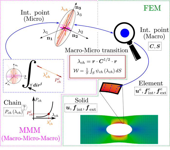
FIGURE 1. On the right side the FEM part (green contour), from bottom to top there are different levels, first at the solid level, the nodal displacement vector, u, the nodal internal forces, fint, and the external nodal forces, fext, are encountered. Second, at the element level, the elemental nodal displacement vector, ue, the elemental nodal internal forces,
In the following sections we introduce the procedure, first using a continuum hyperelastic formulation and then the micromechanical one. We also demonstrate the applicability through an academic example and an example using the well-known Treloar’s rubber.
One way to obtain the displacement-based finite element formulation is through the principle of virtual work, which for the quasi-static case reads δW = δWint − δWext = 0. Considering a conventional FEM discretization and interpolation of the displacement field, both virtual works (internal and external) could also be expressed in terms of the internal and external nodal forces,
where δu and u are the virtual displacement field, and the displacement field, respectively, P, the 1st PK (First Piola-Kirchhoff) stress tensor, b the volumetric forces and t the surface forces. The symbol ⊗ represents the dyadic production, so
As it has already been mentioned, a FEM discretization for the internal force term, ∫ΩP: ∇δudΩ, and the interpolation of the displacement field in the reference unit element,
where all the variables with subscript j are computed in the integration point j. The previous equations can be rewritten doing the sum over the DOF of the element (ndofs = nn × 2 in the 2D solid elements) instead of doing the sum over the nodes:
In Eq. 3, i is the index that runs through the local degrees of freedom in the element, for the cases studied here (2D plane stress problems) i = 1, … , 2nn, δui is the virtual displacement at the local degree of freedom i and
where
Since the PK1 tensor is a two-leg tensor placed in 2 configurations at the same time (material in the right and spatial in the left), it might be more suitable to rewrite the term
In order to simplify the notation we define
To compute the principal stress components of a polymeric and quasi-incompressible material, we assume that the volumetric and deviatoric contributions of the energy can be separated (a typical assumption in quasi-incompressibility),
where Ni are the principal referential directions of deformation,
From the previous equation, the pressure term could be isolated and introduced in the equations for S1 and S2:
Once the principal stretches are known for a particular integration point, the principal PK2 stress components in that same point could be determined through evaluation of the deviatoric contribution derivatives. When the stress tensor has been computed in all the integration points of the element, the internal nodal forces for that element are computed using (Eq. 4). On the other hand, if the functions for the deviatoric contribution derivatives are unknown, a cubic P-Spline local approximation can be employed, see Amores et al. (2019), Eilers and Marx (2021). The B-splines (or its penalized version, P-splines) are one of the approaches for expressing any general function y(x) as the product of a set of known basis functions (cubic in this case),
and for the element local degree of freedom i
which means that every component of the elemental nodal force vector is obtained as the product of a known row multiplied by the unknown vertices, or expressed in a different manner:
where
In case the body forces and the tractions are not zero, the external force vector for each element,
On the previous equations, the reaction forces on the boundary where displacements are imposed are accounted in the traction term, for the sake of simplicity we are going to consider that those nodal reaction forces are known, while this is not typically the case in a experimental setting, instead, the total reaction forces are known rather than the nodal forces. To deal with this fact, 2 different approaches can be followed: 1) take another artificial boundary far enough from the original one in which we can suppose that the reaction force is evenly distributed according to the Saint-Venant’s principle or 2) consider two independent set of equations one for the free dofs and other for the DOF with fixed displacements, in the fixed displacement DOF the resultant of the internal forces equals the reaction force at each of the boundaries.
The problem to solve is an overdetermined linear system of equations
The solution for the previous minimization problem is analytical and result in the mentioned linear system of equations:
As we have already mentioned, one of the advantages of using the P-Spline-based local approximation is that although we do not assume the form of the energy function, additional requirements can be added to the solution, a typical one is smoothness, which can be translated into a penalization on the second order finite differences of the P-spline vertices, if the solution obtained is not monotonically increasing, this property could also be imposed by iterative penalization on the vertices that do not satisfy the condition see Amores et al. (2019), Eilers and Marx (2021). With all the penalizations, the general system of equations to solve would be:
where W is a diagonal matrix that weights the relative importance of the equations in
In this section we are going to demonstrate just the FEM part of the methodology using a P-Spline based approximation for the functions that form the deviatoric continuum free energy. The experimental data is a virtual test (FEM results) of an analytical quasi-incompressible Neo-Hookean model with parameters μ = 3.5 MPa and κ = 1 × 10⁵ MPa. The FEM model employed for the virtual tests is a 2D plate with a hole on plane stress conditions. The solicitation is an imposed displacement in the upper border with u = 4. The dimensions of the plate and the mesh employed in the simulation is shown in Figure 2, the elements are quadratic quadrilaterals with nine integration points. The formulation employed for plane stress in large deformations is detailed in Supplementary Appendix SA, the reader can also find the details about the Neo-Hookean material model in Supplementary Appendix SB. Regarding the software employed, Julia programming language, Bezanson et al. (2017) has been used, in particular the package FerriteFem.jl, see Carlsson and Ekre (2021), for the FEM simulations and Amores (2022) for the P-Splines functionality.
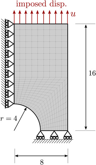
FIGURE 2. FEM model used during virtual tests. The elements employed are quadratic quadrilateral with nine integration points.
A typical assumption made on the phenomenological approach for isotropic incompressible solids is the Valanis Landel decomposition,
Once
With the previous expression, the principal stresses could be written as:
Referring again to Eq. 13, internal nodal forces of the element can be written as the product of a known matrix by a vector of unknown vertices:
Doing the assembly of the internal nodal forces of the elements in the mesh:
From the overdetermined linear system of equations
The number of vertices has to be enough to capture the complexity of the curve, typically nvert = 14 suffice, but additional vertices can be added. If more and more vertices are added, the number of equations required to determine them increases and the problem can become ill-conditioned, this is solved by the smoothing term which adds the information of smooth transition between vertices and links the vertices to its neighbours. In the homogeneous case, just a single equation is obtained for every load/displacement step, therefore, in order to obtain information for the function on the considered domain (from the minimum principal stretch to the maximum principal stretch on the simulation), it would be necessary to sweep a whole range of load/displacement steps. On the other hand, for the non-homogeneous case, in principle, it would be possible to employ just a single load/displacement step if the step under consideration is rich enough (in this case, just the last step, u = 4 was used). In case that additional information is needed to determine the function on the considered range, it is also possible to add more steps between u = 0 and u = 4. Since the initial solution was directly monotonically increasing, Ω1 = 0 and it was not necessary to follow an iterative process,
With the vertices obtained, the P-Spline could be reconstructed and compared to the original one, see Figure 3.
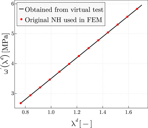
FIGURE 3. Comparison of the Neo-Hookean
Since the function
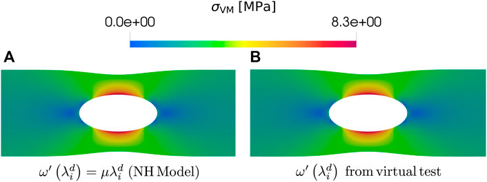
FIGURE 4. Plot comparing the results of σVM for the reference Neo-Hookean continuum model and the reverse-engineered one. (A) σVM using the Neo-Hookean model. (B) σVM using the
In this particular example, the matrix of the system
where C = XTX is the right Cauchy-Green tensor and
In this section the complete methodology described in Section 2 (Macro-Micro-Macro first, FEM second) is demonstrated. In contrast to the procedure described in Section 3.1, here the P-Spline will approximate the derivative of the chain energy function
In Amores et al. (2020) a way was established to compute the strain energy function of the continuum with an homogenization of the micro-structural chain free energy function in polymeric like materials under the assumption of incompressibility (λ1 ⋅ λ2 ⋅ λ3 = 1):
For FEM simulations even pure incompressible solids are simulated with the quasi-incompressible material framework:
in which
The unknown function that will be approximated using P-Splines is
Introducing the expression for
Note that the previous integral in the microsphere is computed by a numerical quadrature,
Looking at the previous matrix equation and using again (Eq. 13), it is straightforward to write the internal vector force for an element as
where
At that point it is important to note that if compared to the procedure followed in Section 3.1, now the internal force term is linked with the unknown vertices that correspond to the constituents behavior at the micro-scale. With that approach we show that scales can be crossed and information in one scale can be pushed up to other scales, that of course taking into account that the macro to micro connection has already been established.
From the overdetermined linear system of equations
The discussion about the number of vertices and steps of load/displacement required in Section 3.1 is also applicable here. In this particular case, just the last step of deformation (u = 8) was used. Again, in case that additional information is needed to determine the function on the considered range, it is also possible to add more steps between u = 0 and u = 8. Since the initial solution was directly monotonically increasing, Ω1 = 0 and it was not necessary to follow an iterative process,
With the vertices obtained, the P-Spline could be reconstructed and compared it to the original one, see Figure 5.
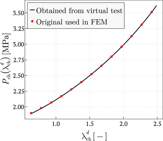
FIGURE 5. Plot comparing
As it is shown in Figure 5, the
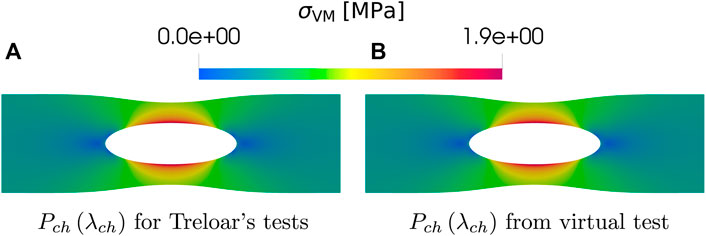
FIGURE 6. Plot comparing the results of σVM for the reference micro-mechanical model in Amores et al. (2020) that uses (Amores et al., 2020, Figure B.1) and the reverse-engineered one described in the article. (A) σVM using the
We have proposed a numerical method for determining both the continuum free energy and the polymer macromolecules behavior from arbitrary non-homogeneous DIC-based tests at the continuum scale. The procedure consists of a combination of our Macro-Micro-Macro approach and a Finite Element model. As a novel contribution of this approach, we show that by crossing scales transferring the microscale unknowns to the finite element formulation it is possible to determine the mechanical chain behavior from non-homogeneous experiments at the continuum scale by simply solving a linear system of equations (i.e., in an even more efficient manner than the subsequent simulations of the polymer behavior). Another key aspect is that Penalized B-splines (P-splines) preserve the general form of the energy function while retaining sufficient tools for enforcing specific desired conditions on the sought functions. The methodology at hand recovers the analytical free energies used as starting point in the virtual tests. Therefore, any finite element simulation performed with the reversed-engineered energy function will provide identical results to the original material model. From the authors perspective, this new approach opens new possibilities for data-driven characterization of the micro-structure from non-homogeneous tests at the macro-scale. Further research has to be conducted to evaluate the generalization of the approach in Amores et al. (2020) to more complex material behaviors from which the applicability of this same methodology has to be assessed.
The raw data supporting the conclusion of this article will be made available by the authors, without undue reservation.
VA: Conceptualization, methodology, software, and writing original draft. FM: Conceptualization, methodology, funding acquisition, and supervision. EC: Methodology and supervision. FC: Conceptualization, methodology, funding acquisition, and supervision. All authors contributed to manuscript revision, read, and approved the submitted version.
 This project has received funding from the European Union’s Horizon 2020 research and innovation programme under the Marie Skłodowska-Curie Grant Agreement No. 101007815.
The authors declare that the research was conducted in the absence of any commercial or financial relationships that could be construed as a potential conflict of interest.
All claims expressed in this article are solely those of the authors and do not necessarily represent those of their affiliated organizations, or those of the publisher, the editors and the reviewers. Any product that may be evaluated in this article, or claim that may be made by its manufacturer, is not guaranteed or endorsed by the publisher.
The Supplementary Material for this article can be found online at: https://www.frontiersin.org/articles/10.3389/fmats.2022.879614/full#supplementary-material
Alastrué, V., Martínez, M. A., Doblaré, M., and Menzel, A. (2009). Anisotropic Micro-sphere-based Finite Elasticity Applied to Blood Vessel Modelling. J. Mech. Phys. Sol. 57, 178–203. doi:10.1016/J.JMPS.2008.09.005
Amores, V. J., Benítez, J. M., and Montáns, F. J. (2019). Average-chain Behavior of Isotropic Incompressible Polymers Obtained from Macroscopic Experimental Data. A Simple Structure-Based WYPiWYG Model in Julia Language. Adv. Eng. Softw. 130, 41–57. doi:10.1016/j.advengsoft.2019.01.004
Amores, V. J., Benítez, J. M., and Montáns, F. J. (2020). Data-driven, Structure-Based Hyperelastic Manifolds: A Macro-Micro-Macro Approach to Reverse-Engineer the Chain Behavior and Perform Efficient Simulations of Polymers. Comput. Structures 231, 106209. doi:10.1016/J.COMPSTRUC.2020.106209
Amores, V. J., Nguyen, K., and Montáns, F. J. (2021). On the Network Orientational Affinity assumption in Polymers and the Micro-macro Connection through the Chain Stretch. J. Mech. Phys. Sol. 148, 104279. doi:10.1016/J.JMPS.2020.104279
Arruda, E. M., and Boyce, M. C. (1993). A Three-Dimensional Constitutive Model for the Large Stretch Behavior of Rubber Elastic Materials. J. Mech. Phys. Sol. 41, 389–412. doi:10.1016/0022-5096(93)90013-6
Bergström, J. S., and Hayman, D. (2016). An Overview of Mechanical Properties and Material Modeling of Polylactide (PLA) for Medical Applications. Ann. Biomed. Eng. 44, 330–340. doi:10.1007/S10439-015-1455-8/TABLES/2
Bezanson, J., Edelman, A., Karpinski, S., and Shah, V. B. (2017). Julia: A Fresh Approach to Numerical Computing. SIAM Rev. 59, 65–98. doi:10.1137/141000671
Chagnon, G., Ohayon, J., Martiel, J.-L., Favier, D., Modeling, D. F. H., Chagnon, G., et al. (2017). “Hyperelasticity Modeling for Incompressible Passive Biological Tissues,” in Biomechanics of Living Organs. Academic Press (Elsevier), 3–30. doi:10.1016/B978-0-12-804009-6.00001-8
Chagnon, G., Rebouah, M., and Favier, D. (2015). Hyperelastic Energy Densities for Soft Biological Tissues: A Review. J. Elast 120, 129–160. doi:10.1007/S10659-014-9508-Z
Crespo, J., and Montáns, F. J. (2018). A Continuum Approach for the Large Strain Finite Element Analysis of Auxetic Materials. Int. J. Mech. Sci. 135, 441–457. doi:10.1016/J.IJMECSCI.2017.11.038
Eggersmann, R., Kirchdoerfer, T., Reese, S., Stainier, L., and Ortiz, M. (2019). Model-Free Data-Driven Inelasticity. Comput. Methods Appl. Mech. Eng. 350, 81–99. doi:10.1016/J.CMA.2019.02.016
Eilers, P. H. C., and Marx, B. D. (2021). Practical Smoothing: The Joys of P-Splines. Cambridge University Press. doi:10.1017/9781108610247
Flaschel, M., Kumar, S., and De Lorenzis, L. (2021). Unsupervised Discovery of Interpretable Hyperelastic Constitutive Laws. Comput. Methods Appl. Mech. Eng. 381, 113852. doi:10.1016/J.CMA.2021.113852
Flory, P. J., and Rehner, J. (1943). Statistical Mechanics of Cross‐Linked Polymer Networks II. Swelling. J. Chem. Phys. 11, 521–526. doi:10.1063/1.1723792
Gent, A. N. (1989). Rubberlike Elasticity-A Molecular Primer, by James E. Mark and Burak Erman, John Wiley & Sons, New York, 1988, 196 Pp. J. Polym. Sci. C Polym. Lett. 27, 405–406. doi:10.1002/POL.1989.140271012
González, D., Chinesta, F., and Cueto, E. (2018). Thermodynamically Consistent Data-Driven Computational Mechanics. Continuum Mech. Thermodyn. 31 (1), 239–253. doi:10.1007/S00161-018-0677-Z
Holzapfel, G. A. (2002). Nonlinear Solid Mechanics: a Continuum Approach for Engineering Science. Meccanica 37, 489–490. doi:10.1023/a:1020843529530
Ibañez, R., Abisset-Chavanne, E., Aguado, J. V., Gonzalez, D., Cueto, E., and Chinesta, F. (2018). A Manifold Learning Approach to Data-Driven Computational Elasticity and Inelasticity. Arch. Computat Methods Eng. 25, 47–57. doi:10.1007/S11831-016-9197-9/FIGURES/11
Ibañez, R., Borzacchiello, D., Aguado, J. V., Abisset-Chavanne, E., Cueto, E., Ladevèze, P., et al. (2017). Data-driven Non-linear Elasticity: Constitutive Manifold Construction and Problem Discretization. Comput. Mech. 60, 813–826. doi:10.1007/S00466-017-1440-1
Khiêm, V. N., and Itskov, M. (2016). Analytical Network-Averaging of the Tube Model:. J. Mech. Phys. Sol. 95, 254–269. doi:10.1016/J.JMPS.2016.05.030
Kirchdoerfer, T., and Ortiz, M. (2016). Data-driven Computational Mechanics. Comput. Methods Appl. Mech. Eng. 304, 81–101. doi:10.1016/J.CMA.2016.02.001
Kirchdoerfer, T., and Ortiz, M. (2018). Data-driven Computing in Dynamics. Int. J. Numer. Meth. Engng 113, 1697–1710. doi:10.1002/NME.5716
Korzeniowski, T. F., and Weinberg, K. (2021). A Multi-Level Method for Data-Driven Finite Element Computations. Comput. Methods Appl. Mech. Eng. 379, 113740. doi:10.1016/J.CMA.2021.113740
Latorre, M., and Montáns, F. J. (2013). Extension of the Sussman-Bathe Spline-Based Hyperelastic Model to Incompressible Transversely Isotropic Materials. Comput. Structures 122, 13–26. doi:10.1016/J.COMPSTRUC.2013.01.018
Latorre, M., and Montáns, F. J. (2014). What-You-Prescribe-Is-What-You-Get Orthotropic Hyperelasticity. Comput. Mech. 53, 1279–1298. doi:10.1007/S00466-013-0971-3
Liu, X., Tao, F., Du, H., Yu, W., and Xu, K. (2020). Learning Nonlinear Constitutive Laws Using Neural Network Models Based on Indirectly Measurable Data. J. Appl. Mech. Trans. ASME 87. doi:10.1115/1.4047036/1083320
Marckmann, G., and Verron, E. (2006). Comparison of Hyperelastic Models for Rubber-like Materials. Rubber Chem. Techn. 79, 835–858. doi:10.5254/1.3547969
Mooney, M. (1940). A Theory of Large Elastic Deformation. J. Appl. Phys. 11, 582–592. doi:10.1063/1.1712836
Moreno, S., Amores, V. J., Benítez, J. M., and Montáns, F. J. (2020). Reverse-engineering and Modeling the 3D Passive and Active Responses of Skeletal Muscle Using a Data-Driven, Non-parametric, Spline-Based Procedure. J. Mech. Behav. Biomed. Mater. 110, 103877. doi:10.1016/J.JMBBM.2020.103877
Nguyen-Thanh, V. M., Zhuang, X., and Rabczuk, T. (2020). A Deep Energy Method for Finite Deformation Hyperelasticity. Eur. J. Mech. - A/Solids 80, 103874. doi:10.1016/J.EUROMECHSOL.2019.103874
Ogden, R. W. (1972). Large Deformation Isotropic Elasticity - on the Correlation of Theory and experiment for Incompressible Rubberlike Solids. Proc. R. Soc. Lond. A. 326, 565–584. doi:10.1098/RSPA.1972.0026
Sáez, P., Alastrué, V., Peña, E., Doblaré, M., and Martínez, M. A. (2011). Anisotropic Microsphere-Based Approach to Damage in Soft Fibered Tissue. Biomech. Model. Mechanobiol 11, 595–608. doi:10.1007/S10237-011-0336-9
Sussman, T., and Bathe, K.-J. (2009). A Model of Incompressible Isotropic Hyperelastic Material Behavior Using Spline Interpolations of Tension-Compression Test Data. Commun. Numer. Meth. Engng. 25, 53–63. doi:10.1002/CNM.1105
Treloar, L. R. G. (1944). Stress-Strain Data for Vulcanized Rubber under Various Types of Deformation. Rubber Chem. Techn. 17, 813–825. doi:10.5254/1.3546701
Zheng, Z., Ye, H., Zhang, H., Zheng, Y., and Chen, Z. (2020). Multi-Level K-D Tree-Based Data-Driven Computational Method for the Dynamic Analysis of Multi-Material Structures. Int. J. Mult. Comp. Eng. 18, 421–438. doi:10.1615/INTJMULTCOMPENG.2020035167
Ω1 Weight matrix for the first differences
Ω2 Weight matrix for the second differences
A Green Lagrange strain tensor
b Volumetric forces
C Right Cauchy Green tensor
D1 First differences matrix
D2 Second differences matrix
fext External nodal forces
fint Internal nodal forces
Ni Principal referential direction of deformation number i
P PK1 (First Piola-Kirchhoff) stress tensor
r Arbitrary direction of the unit sphere in the reference configuration
S PK2 (Second Piola-Kirchhoff) stress tensor
t Surface forces
u Displacement field
ua Displacement vector of node a
W Weight matrix for the system of equation
X Gradient of deformation tensor, X = ∂tx/∂0x
∇ Nabla operator, ∇ = ∂iei
δu Virtual displacement field
δW Virtual work
δWext External virtual work
δWint Internal virtual work
Γ Area in the reference configuraion
κ Bulk modulus
0ξ Local coordinates for the unit reference element
μ Shear modulus
ψch Chain free energy function
□ Volume of the unit reference element
ha Shape function of node a in the reference unit element
J Volume ratio
MSE Mean square error
ndofs Number of DOFs per element
nvert Number of vertices of the BSpline
nel Number of elements
nn Number of nodes
nqp Number of quadrature points per element
nqS Number of quadrature points on the microspheres
Pch Chain mechanical behavior function, Pch = dψch/dλch
ri Director cosine of the vector r with respect to Ni
Si Principal value i of the PK2 stress tensor
wj Quadrature weight for the integration point j of the element
λch Non-affine chain stretch, λch = r ⋅U ⋅ r
λi Principal stretch i
Keywords: hyperelasticity, data-driven modeling, polymers, digital image correlation, machine learning, splines
Citation: Amores VJ, Montáns FJ, Cueto E and Chinesta F (2022) Crossing Scales: Data-Driven Determination of the Micro-scale Behavior of Polymers From Non-homogeneous Tests at the Continuum-Scale. Front. Mater. 9:879614. doi: 10.3389/fmats.2022.879614
Received: 19 February 2022; Accepted: 22 March 2022;
Published: 31 May 2022.
Edited by:
Norbert Huber, Helmholtz-Zentrum Hereon, GermanyReviewed by:
Alexander Lion, Munich University of the Federal Armed Forces, GermanyCopyright © 2022 Amores, Montáns, Cueto and Chinesta. This is an open-access article distributed under the terms of the Creative Commons Attribution License (CC BY). The use, distribution or reproduction in other forums is permitted, provided the original author(s) and the copyright owner(s) are credited and that the original publication in this journal is cited, in accordance with accepted academic practice. No use, distribution or reproduction is permitted which does not comply with these terms.
*Correspondence: Víctor J. Amores, dmljdG9yamVzdXMuYW1vcmVzQHVwbS5lcw==
Disclaimer: All claims expressed in this article are solely those of the authors and do not necessarily represent those of their affiliated organizations, or those of the publisher, the editors and the reviewers. Any product that may be evaluated in this article or claim that may be made by its manufacturer is not guaranteed or endorsed by the publisher.
Research integrity at Frontiers
Learn more about the work of our research integrity team to safeguard the quality of each article we publish.