 Ronak Shoghi
 Alexander Hartmaier
- ICAMS, Ruhr-Universität Bochum, Bochum, Germany
Trained machine learning (ML) algorithms can serve as numerically efficient surrogate models of sophisticated but numerically expensive constitutive models of material behavior. In the field of plasticity, ML yield functions have been proposed that serve as the basis of a constitutive model for plastic material behavior. If the training data for such ML flow rules is gained by micromechanical models, the training procedure can be considered as a homogenization method that captures essential information of microstructure-property relationships of a given material. However, generating training data with micromechanical methods, as for example, the crystal plasticity finite element method, is a numerically challenging task. Hence, in this work, it is investigated how an optimal data-generation strategy for the training of a ML model can be established that produces reliable and accurate ML yield functions with the least possible effort. It is shown that even for materials with a significant plastic anisotropy, as polycrystals with a pronounced Goss texture, 300 data points representing the yield locus of the material in stress space, are sufficient to train the ML yield function successfully. Furthermore, it is demonstrated how data-oriented flow rules can be used in standard finite element analysis.
Introduction
The finite element method is one of the most popular methods used in solid mechanics to solve the nonlinear partial differential equations describing mechanical equilibrium of a solid under arbitrary boundary conditions. The solution of a solid mechanics problem must satisfy equations of equilibrium, compatibility of strains and displacements, and obey the constitutive laws for the materials represented in the model (Chen and Saleeb, 1994; Pian and Wu, 2005). These constitutive equations describe the relationships between stresses and strains, i.e., they quantify the material response under given distortions. In the simplest case of elastic materials, this relationship assumes a linear form in which stress and strain are proportional to each other, as described by Hooke’s law. For nonlinear and irreversible material behavior, as it must be considered for plastic materials, elastic and plastic strains need to be treated by separate constitutive models (Chen and Saleeb, 1994; Bonet and Wood, 1997). While for elastic strains, Hooke’s law is still valid, plastic strains need to be calculated in a way that is consistent with the yield strength and the flow stress observed in tensile tests of the given material. To accomplish this, a yield function is formulated that indicates whether a given stress state results in a linear-elastic material response or whether plastic deformation needs to be considered. In the linear elastic regime, the yield function takes negative values, and it reaches the value zero for those stress tensors for which plastic yielding starts. Hence, the zeros of the yield function can be represented by a hypersurface in stress space, which embodies the convex hull of the stress tensors leading to a linear-elastic material response. In the Voigt notation, the six-dimensional (6D) stress space itself is spanned by the six independent components of the stress tensor, including normal and shear components. In the case of ideal plasticity, this hypersurface in stress space, the so-called yield-locus, remains unchanged by plastic deformation (Chen and Saleeb, 1994). In contrast, in the case of strain hardening, it can change its volume (isotropic hardening), location (kinematic hardening), or shape (distortive hardening) (Helling and Miller, 1987; Kurtyka and Życzkowski, 1996).
This concept of the yield locus as geometrical representation of the yield criterion can also be applied in cases of anisotropic plastic deformation, as it occurs, for example, in polycrystalline metals with specific crystallographic textures. This plastic anisotropy of polycrystals can be described with the crystal plasticity finite element method (CPFEM) (Roters et al., 2011), for an overview, in which plastic slip on the discrete crystallographic slip planes of each grain is considered. Such methods also allow us to study the evolution of textures under large plastic strains (Peranio et al., 2010), where certain crystallographic planes tend to rotate concerning the direction of the highest principal strain and, thus, cause a dynamic change of the crystallographic texture and the resulting plastic anisotropy, which is the origin of distortive hardening in these materials.
While CPFEM methods represent a fundamental way of describing plastic anisotropy of materials, they cause a high numerical effort, limiting their application to relatively small volumes. In the work of Vajragupta et al. (2017), it has been shown that the results of CPFEM calculations can be homogenized by fitting the parameters of an anisotropic yield criterion to data obtained from CPFEM calculation of specific textures. Various formulations of such anisotropic yield criteria have been published in the literature (Karafillis and Boyce, 1993; Cazacu and Barlat, 2001; Banabic et al., 2004). In this work, we refer to the formulation of Hill (Hill, 1948) with six parameters describing the state of anisotropy, which has been suggested as a generalization of the isotropic yield criterion after Huber-Von Mises (Huber, 1904; v Mises, 1913), based on the second invariant of the stress deviator (J2). The corresponding equivalent stress can be compared to the scalar yield stress of the material determined in a uniaxial test. Barlat et al. (2005) suggested a yield function that contains 18 parameters (Yld 2004-18p) based on a linear transformation of the stress deviator.
In more recent approaches, data-driven computational methods have been suggested in the literature to describe anisotropic material behavior. In the data-driven method suggested by Kirchdoerfer and Ortiz (2016), instead of constitutive models for finite element analysis, experimental material data can be used directly to satisfy the required constraints and conservation laws for mechanical equilibrium. In a similar approach, Eggersmann et al. (2019), Eggersmann et al. (2021) have shown that a model-free data-driven formulation of mechanical problems can be achieved. In the work of Chinesta et al. (2017) the data-driven strategy was extended for nonlinear material behavior, which includes not only the plastic strain rate and the rate of accumulated plastic deformation but also the kinematic hardening rate. Another popular approach to develop a data-driven material model is using machine learning algorithms that are capable of handling large data sets. At the same time, they provide the possibility of describing arbitrary mathematical functions, thus relieving the restrictions for closed-form mathematical descriptions of anisotropic yield criteria. Liu et al. (2018) employ a clustering technique to solve the equilibrium equation on clusters of material points with similar mechanical responses. In another approach suggested by Ibañez et al. (2018), manifold learning methods were used to define the constitutive manifold of a given material, allowing the extraction of relevant information directly from large experimental data sets. In Linka et al. (2021), a machine learning-based hyperelasticity model is suggested using a feed-forward neural network trained using experimental data. (Linka et al. (2021) introduced constitutive artificial neural networks to describe hyperelastic material behavior.
Following the method developed in (Hartmaier, 2020), the present work uses Support Vector Classification (SVC) of the elastic and plastic domains in the stress space as a data-oriented yield function. The SVC algorithm is trained by using input data in the form of critical stresses that mark the onset of plastic yielding, thus representing the yield locus in a data-based manner. In this way, a machine learning (ML) yield function is obtained to determine whether a given stress state lies inside or outside the material’s elastic domain. Getting a proper data-based representation of the yield locus as a hypersurface in the 6D stress space can be challenging. This holds in particular if the training data is generated by numerically expensive methods as CPFEM. Hence, in this work, we will use simpler methods for the generation of various data sets that are the basis for the development of an optimal strategy to distribute the training data points over the entire yield locus with as small as possible data sets. Based on these training data, an accurate ML yield locus, i.e., the hypersurface in the stress space on which plastic deformation occurs, can be reconstructed from the SVC in the form of a convolutional sum over a kernel function, from which the gradient on this yield locus can be conveniently calculated. Therefore, the standard formulations of continuum plasticity, as the return mapping algorithm, can be applied in the usual way to finite element analysis (FEA). Thus, it is demonstrated that the new ML yield function can replace conventional FEA flow rules.
Methods
Machine Learning Flow Rule
The elastic-plastic deformation of a material can be described using stress and strain tensors denoted with
In the Voigt notation, the symmetric tensor is defined by its six independent components as
where
and plastic deformation sets in at
In this yield function, the anisotropy of the material’s flow behavior is described in a Hill-like approach, where the parameters
when
The gradient of the yield function with respect to the stress components is needed for calculating the plastic strain increments in the return mapping algorithm of continuum plasticity and can be evaluated analytically as
In the case of isotropic plasticity, i.e.,
Where
Data-Oriented Yield Function
In the data-oriented approach followed in this work, the yield function
The support vector method aims to construct a classifier in form
where
Since the ML yield function is defined as convolution sum over support vectors, the gradient to the SVC decision function can be calculated as
When using the RBF kernel for training,
A high training quality relies on providing sufficient training points on the yield locus, as the SVM algorithm creates support vectors only in the areas covered by training points. While in previous work (Hartmaier, 2020) only the three-dimensional space of principal stresses was considered, where the coverage of the yield locus with data points is a rather trivial task, it is quite a challenge to create data points efficiently in the full 6D stress space. An optimal strategy to create as few as possible data points representing the yield locus in the best possible way is necessary, particularly when data points are created with numerically expensive methods such as CPFEM.
Data-Generation Model
Creating a set of yield stresses in the full stress space that serves as the ground truth is required to train the ML yield function. In a first step, unit stresses need to be generated that define the load cases, i.e., the directions in which the load is applied. Then, each unit stress is proportionally increased until the value of the yield function
Finally, the full set of stress tensors at the onset of plastic yielding represents the ground truth for the training of the ML yield function (Hartmaier, 2020). The task of finding the zeros of the yield function, i.e., the critical stress tensor at the onset of plastic yielding, for each load case needs to be done by a fundamental method, such as CPFEM or mechanical testing that captures the yielding behavior of the material under investigation. Hence, the effort for funding this ground truth is a considerable task that represents the major effort for training an ML flow rule. Thus, finding an optimal strategy for creating the unit stresses is the primary goal of this work. The starting point is creating different distributions of unit stresses on the surface of a unit sphere in a full 6D stress space. After this, the quality of the ML yield criterion resulting from the training with these data points is verified to identify the optimal strategy for data generation.
There are different methods for distributing points on the surface of a unit sphere, but not all of them can be extended to dimensions higher than 3. Different algorithms have been proposed to solve the problem of distributing points uniformly over the surface of a unit sphere in higher dimensional spaces because it is a common but highly non-trivial task with many applications in science and engineering. In many proposed solutions, the initial idea is to uniformly distribute points over a rectangular area that is then mapped to a sphere using the cylindrical projection (Hannay and Nye, 2004). In the next part, four different methods are introduced and the dimensions where they can be used are investigated.
One of the most common and simple methods for distributing points on a 3-dimensional sphere is based on the Fibonacci lattice. Based on the work of Marques et al. (2013), Fibonacci lattice points are constructed through a mapping process from the unit square to the unit sphere. A Fibonacci lattice in the unit square is a set
where
given by the polar angle
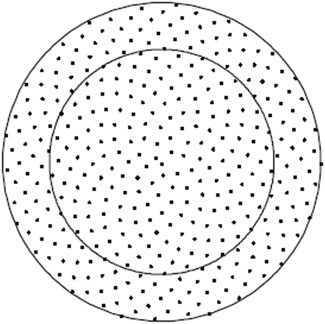
FIGURE 1. Equal area north pole projection of points on the surface of a sphere (Hannay and Nye, 2004).
As
is obtained due to the periodicity of the spherical coordinates (Marques et al., 2013). This relation can be exploited to release the requirement that the number of points has to be a Fibonacci number by defining the coordinates of a spherical point set with an arbitrary, but sufficiently large number
Based on these angles, the cartesian coordinates of the set of equally distributed points on the 3D unit sphere can be calculated as
The even arrangement of points divides the sphere into equal-area spherical rings due to the area-preserving property of the Lambert map. In this arrangement, each ring contains a single lattice node (Swinbank and James Purser, 2006; González, 2010; Marques et al., 2013). A major disadvantage of this formulation for finding equally distributed points on a sphere based on Fibonacci lattice points is that it cannot be extended directly to dimensions higher than 3.
To overcome this limitation, Marsaglia (1972) has suggested a method that allows the selection of uniformly distributed points on the surface of a 4D-sphere. This method is conducted by picking two points as
have a uniform distribution on the surface of a 4D hypersphere. However, this method does not generalize to higher dimensions like the Fibonacci lattice.
Another method that can be used even in higher dimensions is the spherical code problem. In this method, the main goal is distributing
The most promising method which can be used for distributing points on the d-dimensional surface of the sphere
For introducing this method, a polar coordinate system is defined by
For calculating the PDF, we assume that the data drawn from a particular distribution are independent and identically distributed. If we consider a vector
Considering Eqs 21, 22 and based on the assumption that the angles are independently distributed, the d-dimensional PDF can be written as (Raychaudhuri, 2008).
Based on the work of Cai et al. (2013), when the variable
Once the distribution is known for each
If we consider X as the continuous random variate that we want to generate, it will follow
which satisfies
If
where
where
And the angles are given by
This method can be used for recursively creating uniformly distributed points in 6- or even higher-dimensional spaces. The points are distributed such that the distance to the nearest neighbors for each point is maximum. Since the points are constructed to lie on the surface of a unit sphere, the distance of each point to the center of the sphere is unity.
Validation of Uniform Distribution of Data Points
The inverse transform method mentioned in the previous section has been implemented in a python code that is freely available within the Python package “pyLabFEA” (Hartmaier et al., 2022) from a public repository. Using this algorithm, any desired number of points can be distributed uniformly on the surface of a d-dimensional sphere. In Figure 2, 400 points were distributed uniformly on the surface of a unit sphere in 3D space.
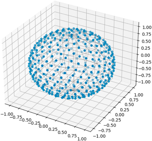
FIGURE 2. 400 points generated uniformly on the surface of a sphere in 3-dimensional space using the combination of Monte Carlo theory and Fibonacci spiral principle.
To test the uniformity of this data generation method, 400 points were distributed on the surface of a hypersphere in 6D space. The average distance from each point to its five nearest neighbors was calculated. The distribution of these distances can be seen in Figure 3A. For comparison, 400 points were generated randomly, and the same average neighboring distance was calculated and is shown in Figure 3B. The random points were generated using the random function available in the NumPy (Harris et al., 2020) package in python.
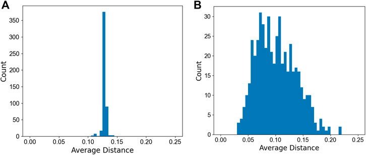
FIGURE 3. Distribution of average distances for five nearest neighboring points of (A) uniform and (B) randomly distributed points on the surface of the unit sphere in 6D space. The total number of points is 400.
It is seen that the method laid out here can create any number of data points that are uniformly distributed on a surface of a d-dimensional unit sphere in the sense that the mutual distance of any two points is maximized and the average distances for K nearest neighbors are at the same range. This method will be used in the following to create the data points for training an ML yield criterion.
Optimal Strategy for Data Generation
In order to find an optimal strategy for selecting a set of training data points, in the following, various data sets will be created with uniform and random distributions and for different sub-spaces of the full stress space. The training results for the different sets are evaluated concerning different error measures, and thus, a strategy to find the smallest possible training data set that provides the desired accuracy of the result is developed.
Since the training data points need to be generated as stress tensors lying on the yield locus of material, we define a reference material with Hill-type anisotropy with the parameters given in Table 1. Using such a relatively simple material model with a simple yield criterion defined in Eq. 2, allows us to generate the training data sets with a minimum effort. This is beneficial for developing an optimal strategy for generating data sets for materials with significant plastic anisotropy. Afterward, it is verified that the training strategy also produces good results for more severe cases of anisotropy as they can be seen in CPFEM results or described by Barlat-type yield criteria to demonstrate the general applicability of the developed method.
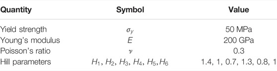
TABLE 1. Elastic and plastic material parameters define the reference material with Hill-like anisotropy in plastic flow behavior. For simplicity, ideal plasticity with no work hardening is considered in this work.
The described reference material is used for creating training data for machine learning algorithms. This is accomplished by first creating unit stresses according to various schemes. Then each unit stress is increased proportionally until the yield function of this stress tensor is zero, i.e., when plastic yielding starts for this specific load case. The full set of stress tensors at the onset of plastic yielding represents the yield function in a data-oriented way and, thus, forms the ground truth for the training of the ML yield function. After this, the ML yield function in form of a Support Vector Classifier (SVC) is trained based on this data set.
As will be seen later, it is necessary to create unit stresses that combine load cases in the full 6D stress space and load cases with purely normal stresses, representing a 3D subspace of the full stress space. For training sets with only 6D load cases, the normal stress space is grossly under-represented with yields a very poor training result. This reflects the fact that the Voigt representation of the symmetric (3 × 3) stress tensor as vector of its six independent components does not fully represent the tensorial properties of the stress as, for example, the existence of a transformation into a diagonal tensor by a rotation of the coordinate system. Hence, the combination of 3D and 6D stresses reflects the tensorial properties of the stress tensor better. The optimal combination of these load cases will be investigated in the second step together with the optimization of the size of the training set.
Uniform Versus Random Training Data Sets
In the first step to develop an optimal training strategy, we compare the results from training with uniformly and randomly distributed training points. For training, 400 load cases have been genertaed, including 350 load cases in full stress space and 50 load cases in principal space. Since the success of the training procedure depends critically on the hyperparameters, the optimal hyperparameters for the SVC were selected using a grid search algorithm for each data set.
For uniformly distributed load cases, the result of SVC training with the hyperparameters
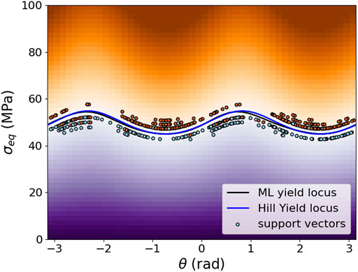
FIGURE 4. The plot of trained SVM classification with uniformly distributed training data in cylindrical coordinates on the
For comparison, the training was done with the same number of load cases, i.e., a total of 400 with 350 in 6D stress space and 50 in normal stress space, that were generated from a random distribution. The optimal hyperparameters for this case were identified as
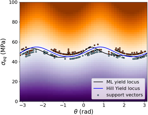
FIGURE 5. The plot of trained SVM classification with randomly selected training data in cylindrical coordinates on the
To further quantify the results of the training procedure, both ML yield functions are verified by comparison with the analytical yield function for random stress tensors in the vicinity of the yield locus. The confusion matrices in Figures 6, 7 summarize the classification performance of both yield functions concerning the same test data in the form of a two-dimensional matrix, indexed in one dimension by the object’s true class and in the other dimension by the class assigned by the classifier. In this context, the four cells of the matrix are designated as true positives (TP), false positives (FP), true negatives (TN), and false negatives (FN) (Shultz et al., 2011).
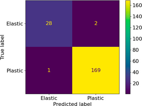
FIGURE 6. Confusion matrix for uniformly distributed load cases.
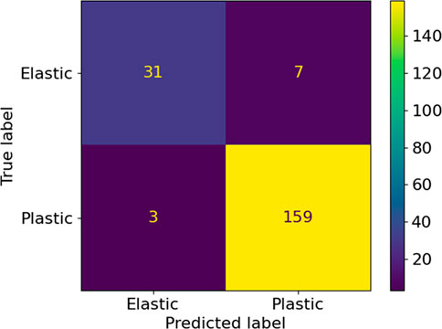
FIGURE 7. Confusion matrix for randomly distributed load cases.
The classification performance can further be quantified in terms of four classification results, as
The summary of metrics for uniform and randomly distributed load cases are given in Table 2. It is concluded that uniformly distributed training data results in a significantly higher quality of the training of the ML yield function. Hence, in the remainder of this work, only this method will be further investigated.
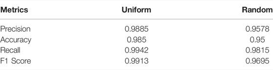
TABLE 2. Summary of the metrics for uniform and random load cases indicate the quality of training.
Optimal Number and Structure of Load Cases
After finding the proper strategy for creating unit stresses uniformly distributed in the stress space, the next step is to find the optimal size for it. Besides the quality, the quantity of training data plays a vital role in the performance of any machine learning model. Small training data sets result in low training accuracy and lack of precision, and a very big training size may lead to overfitting and the problem that the model cannot generalize well to new data. In this context, it is also important to find the optimal ratio of unit stresses in the full 6D stress space and purely normal stresses in the 3D sub-space.
In the first step for finding the proper ratio between 6D and 3D load cases, training was done for a fixed number of 300 load cases and different ratios of 1:2, 1:1, 1.5:1, 2:1, 2.5:1, and 3:2. and the confusion matrix and the training metrics were compared in each case. The corresponding plots can be seen in Figure 8. After training, the precision and mean absolute error were calculated and compared in different ratios of unit load cases in full stress space and the extra cases at principal stress space, the ratio of 2:1 for 6D:3D load cases have highest precision and the lowest mean absolute error (MAE). Mean Absolute error measures the average magnitude of error which quantifies the difference between prediction and the actual observation which can be defined as:
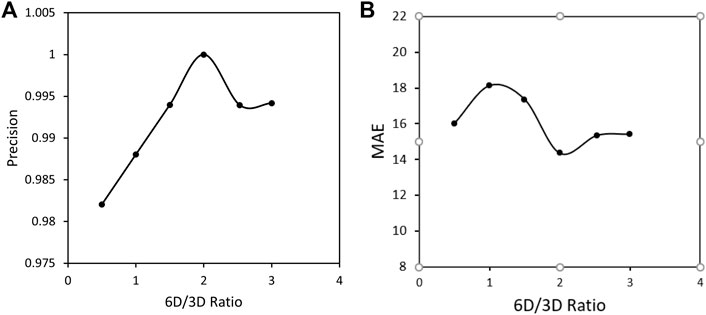
FIGURE 8. (A) Precision and (B) Mean Absolute error after training with total number of 300 load cases in different ratios of load cases in full stress space and extra cases in principal space.
At the next step for finding the optimal training size, the training was done for different total numbers of uniformly distributed load cases with a fixed ratio of 2:1 for 6D to 3D load cases. The comparison is again made based on the precision calculated from the confusion matrix and the MAE, Figure 9. It is seen that a number of 300 is the optimal size for the set of training data with the lowest mean absolute error and a high precision after training. It can be seen that an increasing number of data points leads to an increasing MAE, possibly due to overfitting. Furthermore, the precision does not have a uniform trend with an increasing number of data points such that we conclude that 300 data points is the optimal value, which still allows an efficient data generation process.
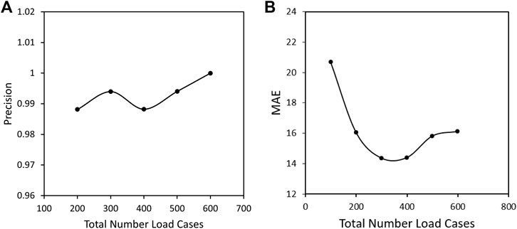
FIGURE 9. (A) Precision and (B) Mean Absolute error after training with different number of load cases and a fixed ratio of 2:1 for 6D to 3D load cases in full stress space and extra cases in principal space.
The resulting ML yield function, trained with the optimized training set of 300 uniformly distributed load cases, is visualized in Figure 10. The optimal hyperparameters for the SVC algorithm have been determined as
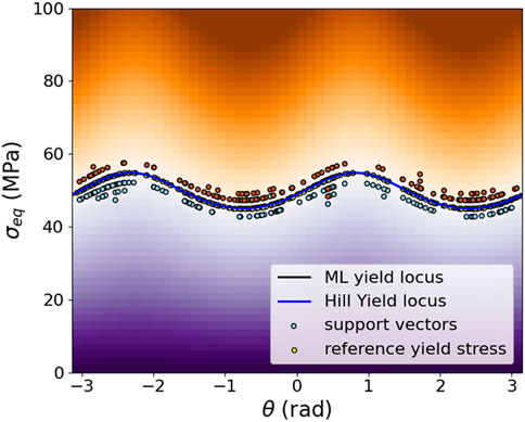
FIGURE 10. Plot of trained SVM classification with optimized training size and ratio in cylindrical coordinates on the
The quality of the ML flow rule training with the optimized data set is further verified by comparing the results of the ML yield function to the known reference values for random stresses in the vicinity of the yield locus. The confusion matrix and the performance metrics were calculated and shown in Figure 11, and Table 3. Comparing to Figures 6, 7 and Table 2 again indicates a better performance after optimization.
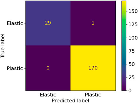
FIGURE 11. Confusion matrix for 300 load cases and the ratio of 2:1 between 6D and 3D load cases.

TABLE 3. Summary of the metrics for 300 with the ratio of 2 between 3D and 6D load cases.
Application of Trained Machine Learning Yield Functions in Finite Element Analysis
Hill-Type Anisotropy
To demonstrate the capabilities and the accuracy of the trained ML yield function, in the first step a finite element analysis (FEA) of a simple 4-element 2D plane-stress model under four load cases has been performed: 1) uniaxial stress in the vertical direction, 2) uniaxial stress in the horizontal direction, 3) equibiaxial strain, and 3) pure shear strain. The numerical simulations shown in this work have been completed with the open-source package pyLabFEA (Hartmaier et al., 2022). All examples of this work are also provided as python code and a Juypter notebook in this public repository. The return mapping algorithm used to calculate the plastic strain increments based on the ML yield function and its gradient, defined in Eqs 12, 14, respectively, has been described in detail in (Suykens and Vandewalle, 1999). In that work, also the full details of the finite element model to evaluate the given load cases are provided. To estimate the accuracy of the ML yield function, its results are compared to the ones obtained from the same model with a Hill-type reference material with elastic-ideal plastic behavior and an analytically defined yield function, Eq. 2. The material parameters for this reference material are given in Table 1. As described above, the ML yield function has been trained to a data set of 300 stress tensors lying on the yield locus of this reference material. The equivalent yield stresses resulting from the FEA under the four given load cases are summarized in Table 4, where it is seen that the error of the ML yield function is only on the order of 0.1%. The resulting curves for equivalent stress versus equivalent strain for each material under the different load cases are plotted in Figure 12, where the elastic-ideal plastic material behavior of both materials is verified for total equivalent strains of up to 1%. Note that the equivalent J2 stress is plotted for both materials because the Hill-type equivalent stress defined in Eq. 3 depends on material parameters that are typically unknown when working with data-based yield functions.
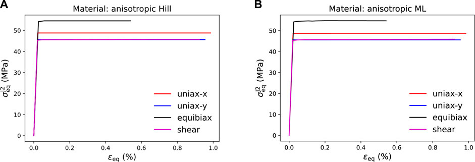
FIGURE 12. Stress-strain curves obtained for elastic-ideal plastic material behavior under the loading conditions specified in the legend. (A) Equivalent J2 stress vs. equivalent total strain for Hill-type yield function, (B) Equivalent J2 stress vs. equivalent total strain for ML yield function.
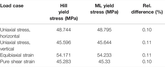
TABLE 4. Yield stress obtained for a Hill-type reference material with analytical yield function and a material with an ML yield function trained to data from the reference material under four specified load cases.
During the plastic deformation of materials with ideal plasticity, it is expected that the flow stresses remain on the yield locus, as the material does not support higher equivalent stresses. In Figure 13, the flow stresses for Hill and ML cases are plotted in the space of the non-zero principal stresses of the plane stress model, together with the yield locus in this slice of the stress space. It is seen that all flow stresses, in fact, remain on the yield locus. Furthermore, it is seen that under stress-controlled boundary conditions, i.e., uniaxial stress in the horizontal or vertical direction, the flow stresses remain constant, whereas, under strain-controlled boundary conditions, the response stress of the anisotropic material is subject to changes. A comparison of this evolution of the flow stress tensor under strain-controlled deformation for the analytical Hill-type yield function and the ML yield function exhibits that both solutions are in very good agreement, demonstrating the accuracy and numerical stability of the ML flow rule even under finite plastic strains.
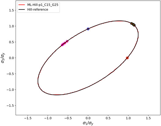
FIGURE 13. The two non-zero principal values of the flow stresses (colored circles) and yield loci of the trained ML flow rule (red line) and the Hill-type reference material (black line) are plotted for four different load cases of the 2D plane stress model. The large colored circles represent the flow stresses resulting from the ML yield function, and the small yellow circles show flow stresses from the analytical Hill-type yield function.
In a second step, the ML yield function is tested under a more complex state of deformation. This is accomplished by performing the FEA of a plane-strain model under uniaxial strain with laterally free boundaries. The three sections of the model are given by a square-shaped elastic inclusion in the middle of a matrix that is vertically split up into the reference material and the ML material, Figure 14. As the ML material is trained to have identical material properties as the reference material, the matrix is expected to show a mirror-symmetric state of deformation. The linear-elastic inclusion is rather compliant, with Young’s modulus of
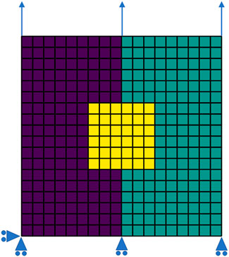
FIGURE 14. A plane strain model with three sections: (i) linear elastic (yellow), (ii) elastic, ideal-plastic reference material with analytic Hill-type yield function (purple), and (iii) elastic, ideal-plastic material with ML yield function (green). The elements forming a regular mesh are indicated as well as the imposed displacements at the boundary.
Figure 14A shows the resulting equivalent stress for each finite element. It is apparent that qualitatively a symmetrical stress state in the different materials is reached. However, quantitatively, the equivalent stresses differ because in the region with the Hill-type material (left-hand-side), the equivalent stress as defined in Eq. 3 is plotted, whereas in the region with the ML material (right-hand-side) the J2 equivalent stress is plotted, which can also be calculated from Eq. 3 when the Hill parameters are set
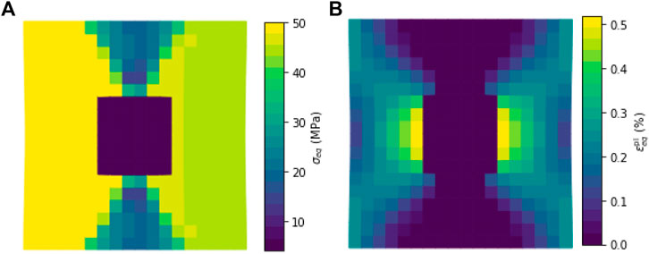
FIGURE 15. Resulting equivalent stress (A) and equivalent plastic strain (B) within the three sections of the model given in Figure 14.
Barlat-Type Anisotropy
After verifying the accuracy and robustness of the ML yield function for cases of Hill-type plastic anisotropy, it is tested here under a more demanding kind of anisotropic behavior, given by a material with a Barlat-type yield function (Yld 2004-18p) (Barlat et al., 2005). The material parameters given in Table 5 have been chosen to mimic a polycrystal with a strong Goss texture, which represents a rather severe case of anisotropic yielding behavior.
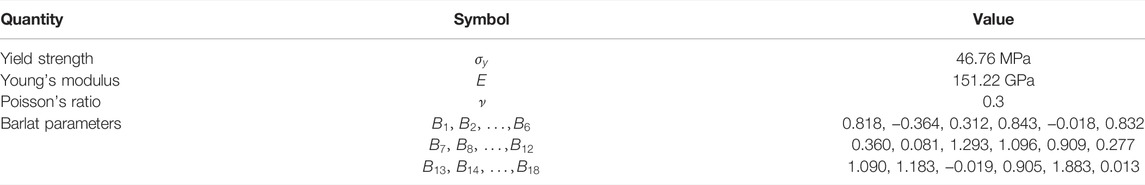
TABLE 5. Material parameters for the Barlat-type reference material, mimicking the plastic anisotropy of a Goss-textured polycrystal.
Following the workflow developed above, in the first step, a set of 300 stress tensors on the yield locus of the Barlat-type reference model is generated. These training stresses are again produced by generating 200 unit stresses as load cases that are uniformly distributed in the 6D stress space and 100 load cases uniformly distributed in the 3D sub-space of normal stresses. Then, these unit stresses are increased proportionally until the zero of the Barlat yield function Yld 2004-18p (Barlat et al., 2005) is reached. The python code for this example is also provided in the pyLabFEA package (Hartmaier et al., 2022). With this training data set, representing the yield locus of the Barlat-type reference material, the ML yield function is trained with the same hyperparameters as given above, i.e.,
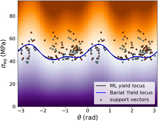
FIGURE 16. Plot of trained ML yield function (black line), the analytic Barlat yield function (blue line) and the support vectors (circles) in cylindrical coordinates on the
The quality of the ML yield function training is further quantified by comparing the signs of the values of the analytical yield function and the ML yield function for 200 random stress tensors in the vicinity of the yield locus. The corresponding confusion matrix is plotted in Figure 17, and the summary of the metrics indicating the high quality of the training result is summarized in Table 6. This analysis confirms that the ML yield function describes the Baralat-type reference material with very high accuracy.
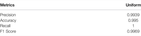
TABLE 6. Summary of the metrics for 300 with a ratio of 2 between 3D and 6D load cases for Trained ML yield function.
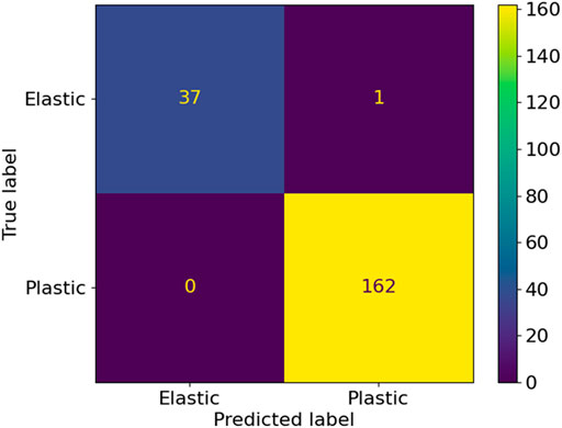
FIGURE 17. Confusion matrix comparing the trained ML yield function and the reference Barlat-type yield function for 200 random stress tensors in the vicinity of the yield locus.
With this trained ML yield function, the same FEA cases as above have been performed to demonstrate the stability of the ML yield function even for a more severe plastic anisotropy. After training, the stress-strain curves are plotted as J2 equivalent stress vs. equivalent total strain in four load Figure 18A cases as shown in Figure 18A. Also, the flow stresses resulting from FEA are plotted in Figure 18B, and they all lie on the ML yield locus as expected for ideal plasticity. Furthermore, it is seen again that for the strain-controlled boundary conditions, the stress tensors change during the plastic deformation. This behavior has already been observed for the Hill-type plastic anisotropy, but it is even more pronounced in this case. Note that for the case of equibiaxial strain, the stresses evolve into a “corner” of the yield locus, which causes a significant increase in the equivalent stress that is also seen in the corresponding stress strain curve for this load case.
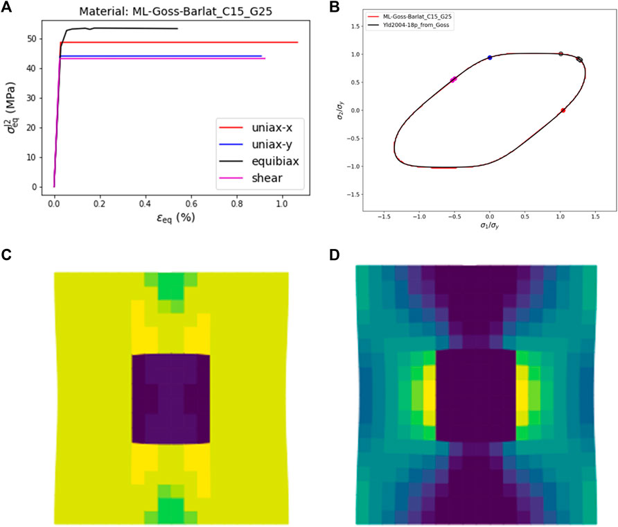
FIGURE 18. (A) Equivalent J2 stress vs. equivalent total strain curves obtained for elastic-ideal plastic material behavior under the loading conditions specified in the legend for the rained ML yield function; (B) yield loci of ML and Barlat-type materials and the flow stresses obtained from the load cases in (A) plotted as principal stresses; (C) equivalent J2 stress; and (D) equivalent plastic strain resulting from the 2D plane strain model with a square-shaped elastic inclusion in the center.
Furthermore, in Figure 18, the equivalent stress Figure 18C and the equivalent plastic strain Figure 18D for a model with a square-shaped elastic inclusion and an elastic-ideal plastic matrix represented by the ML yield function are illustrated to demonstrate the numerical stability of the ML flow rule even in cases of heterogeneous deformation patterns.
Conclusion
In this work, an optimized procedure to generate a data-based description of the yield function of an arbitrary material has been developed. Conventionally, the yield function is based on the concept of the equivalent stress and indicates whether the material response to an applied stress tensor results in linear elastic material response, indicated by a negative value of the yield function, or rather in plastic yielding of the material when the yield function is zero or positive. Mathematically, the zeros of the yield function constitute a hypersurface in stress space, the so-called yield locus, that separates elastic and plastic domains. Since the stress space is 6-dimensional and spanned by the six independent normal and shear components of the stress tensor, it is essential to find an optimal way for sampling this hypersurface with as few as possible data points. Each data point represents a stress tensor at which the material starts to yield plastically, and generating such data requires either numerically expensive approaches such as crystal plasticity finite element methods or laborious mechanical testing under multi-axial loading conditions or a combination of both.
In a first step, a numerical method has been introduced that allows a uniform sampling of the yield locus in a six-dimensional stress space. The main idea behind this method is to proportionally increase uniformly distributed unit stresses until the criterion for plastic yielding is reached for each loading direction. Finding a uniform distribution of arbitrarily many points on the surface of a unit sphere in more than three dimensions is, however, a highly non-trivial task. The solution suggested in this work combines ideas of Monte Carlo sampling and choosing regularly distributed sampling points in higher-dimensional spaces based on the Fibonacci sequence. To sample a higher dimensional unit sphere uniformly, the probability distribution function of its surface needs to be defined in Cartesian coordinates, and then the cumulative distribution function and its inverse need to be computed. Based on this inverse function, a mapping algorithm is defined by which random numbers from the unit interval can be distributed uniformly on the hypersphere. If Fibonacci-like points are mapped accordingly, instead of random numbers, it can be shown that the mutual distance between any two sampling points on the surface of the hypersphere is rather constant and maximized compared to randomly distributed points. It is demonstrated in this work that such a uniform distribution of stress tensors in the 6-dimensional stress space is superior to purely random sampling.
In the next step, this data-oriented description of the yield locus is used as the basis for training of a support vector classifier (SVC) that takes an arbitrary stress tensor as input and predicts whether the material response to this stress is elastic or plastic. In earlier work (Hartmaier, 2020), it has been shown for purely normal stresses how plasticity in the framework of finite element analysis (FEA) can be described based on such trained SVC. Here, this formulation is generalized to the full 6-dimensional stress space, and it is demonstrated that SVC can be trained to predict the behavior of classical yield functions, like Hill or Barlat-type yield functions, with very high accuracy, even for a very significant plastic anisotropy.
As for any machine learning (ML) algorithm, providing high-quality training data is of great importance, as training with smaller sets of proper data will result in a better training success than larger sets of poor data. After finding a suitable way to distribute training data uniformly in stress space, it was found that an appropriate ratio of normal stresses and stresses in the full 6-dimensional stress space is necessary because otherwise, the normal stresses are under-represented. It is demonstrated that a ratio of 1:2 for normal stresses and full stresses represents the tensorial properties of the yield stress in the best way. It is also concluded that 300 data points in the form of stress tensors on the yield locus are sufficient to train the ML yield function with high accuracy, even in cases of severe plastic anisotropy. The thus-trained ML yield functions have been shown to produce accurate and stable numerical solutions in FEA.
To further expand the applicability of ML yield functions in FEA, microstructural parameters like crystallographic texture or grain size and morphology can be included in the input data for the training of the ML yield function, besides the purely mechanical data used in this work. Furthermore, it is crucial to develop a proper data-oriented formulation of work hardening and history-dependent material behavior in the next step.
Data Availability Statement
The original contributions presented in the study are included in the article/Supplementary Material, further inquiries can be directed to the corresponding author.
Author Contributions
Both authors have contributed equally to the work.
Conflict of Interest
The authors declare that the research was conducted in the absence of any commercial or financial relationships that could be construed as a potential conflict of interest.
Publisher’s Note
All claims expressed in this article are solely those of the authors and do not necessarily represent those of their affiliated organizations, or those of the publisher, the editors and the reviewers. Any product that may be evaluated in this article, or claim that may be made by its manufacturer, is not guaranteed or endorsed by the publisher.
Acknowledgments
RS gratefully acknowledges helpful discussions on the mathematical problems with Erik Brinkman. AH gratefully acknowledges funding by the Deutsche Forschungsgemeinschaft (DFG, German Research Foundation)—Project-ID 190389738—TRR 103.
References
Banabic, D., Kuwabara, T., Balan, T., and Comsa, D. S. (2004). An Anisotropic Yield Criterion for Sheet Metals. J. Mater. Process. Technol. 157-158, 462–465. doi:10.1016/j.jmatprotec.2004.07.106
Barlat, F., Aretz, H., Yoon, J. W., Karabin, M. E., Brem, J. C., and Dick, R. E. (2005). Linear Transfomation-Based Anisotropic Yield Functions. Int. J. Plasticity 21, 1009–1039. doi:10.1016/j.ijplas.2004.06.004
Bonet, J., and Wood, R. D. (1997). Nonlinear Continuum Mechanics for Finite Element Analysis. Cambridge: Cambridge University Press. Available at: https://books.google.de/books?id=ORmLdrq1fI8C.
Buddenhagen, J., and Kottwitz, D. A. (2001). Multiplicity and Symmetry Breaking in (Conjectured) Densest Packings of Congruent Circles on a Sphere. Preprint. Available at: https://www.researchgate.net/publication/248871642_Multiplicity_and_Symmetry_Breaking_in_Conjectured_Densest_Packings_of_Congruent_Circles_on_a_Sphere.
Cai, T., Fan, J., and Jiang, T. (2013). Distributions of Angles in Random Packing on Spheres. J. Mach. Learn. Res. 14, 1837–1864.
Cazacu, O., and Barlat, F. (2001). Generalization of Drucker's Yield Criterion to Orthotropy. Maths. Mech. Sol. 6, 613–630. doi:10.1177/108128650100600603
Chen, W. F., and Saleeb, A. F. (1994). Constitutive Equations for Engineering Materials. Amsterdam, Netherlands: Elsevier. Available at: https://books.google.de/books?id=P91IAQAAIAAJ.
Chinesta, F., Ladeveze, P., Ibanez, R., Aguado, J. V., Abisset-Chavanne, E., and Cueto, E. (2017). Data-driven Computational Plasticity. Proced. Eng. 207, 209–214. doi:10.1016/j.proeng.2017.10.763
Eggersmann, R., Kirchdoerfer, T., Reese, S., Stainier, L., and Ortiz, M. (2019). Model-free Data-Driven Inelasticity. Comput. Methods Appl. Mech. Eng. 350, 81–99. doi:10.1016/j.cma.2019.02.016
Eggersmann, R., Stainier, L., Ortiz, M., and Reese, S. (2021). Model-free Data-Driven Computational Mechanics Enhanced by Tensor Voting. Comput. Methods Appl. Mech. Eng. 373, 113499. doi:10.1016/j.cma.2020.113499
González, Á. (2010). Measurement of Areas on a Sphere Using Fibonacci and Latitude–Longitude Lattices. Math. Geosci. 42, 49–64.
Hannay, J. H., and Nye, J. F. (2004). Fibonacci Numerical Integration on a Sphere. J. Phys. A: Math. Gen. 37, 11591–11601. doi:10.1088/0305-4470/37/48/005
Harris, C. R., Millman, K. J., van der Walt, S. J., Gommers, R., Virtanen, P., Cournapeau, D., et al. (2020). Array Programming with NumPy. Nature 585, 357–362. doi:10.1038/s41586-020-2649-2
Hartmaier, A. (2020). Data-oriented Constitutive Modeling of Plasticity in Metals. Materials 13, 1600. doi:10.3390/ma13071600
Hartmaier, A., Menon, S., and Shoghi, R. (2022). Python Laboratory for Finite Element Analysis (PyLabFEA). doi:10.5281/zenodo.5913365
Helling, D. E., and Miller, A. K. (1987). The Incorporation of Yield Surface Distortion into a Unified Constitutive Model, Part 1: Equation Development. Acta Mechanica 69, 9–23. doi:10.1007/bf01175711
Hill, R. (1948). A Theory of the Yielding and Plastic Flow of Anisotropic Metals. Proc. R. Soc. Lond. Ser. A. Math. Phys. Sci. 193, 281–297.
Ibañez, R., Abisset-Chavanne, E., Aguado, J. V., Gonzalez, D., Cueto, E., and Chinesta, F. (2018). A Manifold Learning Approach to Data-Driven Computational Elasticity and Inelasticity. Arch. Computat Methods Eng. 25, 47–57. doi:10.1007/s11831-016-9197-9
Karafillis, A. P., and Boyce, M. C. (1993). A General Anisotropic Yield Criterion Using Bounds and a Transformation Weighting Tensor. J. Mech. Phys. Sol. 41, 1859–1886. doi:10.1016/0022-5096(93)90073-o
Kirchdoerfer, T., and Ortiz, M. (2016). Data-driven Computational Mechanics. Comput. Methods Appl. Mech. Eng. 304, 81–101. doi:10.1016/j.cma.2016.02.001
Kroese, D. P., and Rubinstein, R. Y. (2012). Monte Carlo Methods. Wires Comp. Stat. 4, 48–58. doi:10.1002/wics.194
Kurtyka, T., and Życzkowski, M. (1996). Evolution Equations for Distortional Plastic Hardening. Int. J. Plasticity 12, 191–213. doi:10.1016/s0749-6419(96)00003-4
Linka, K., Hillgärtner, M., Abdolazizi, K. P., Aydin, R. C., Itskov, M., and Cyron, C. J. (2021). Constitutive Artificial Neural Networks: A Fast and General Approach to Predictive Data-Driven Constitutive Modeling by Deep Learning. J. Comput. Phys. 429, 110010. doi:10.1016/j.jcp.2020.110010
Liu, Z., Kafka, O. L., Yu, C., and Liu, W. K. (2018). “Data-driven Self-Consistent Clustering Analysis of Heterogeneous Materials with crystal Plasticity,” in Adv. Comput. Plast. (Berlin, Germany: Springer), 221–242. doi:10.1007/978-3-319-60885-3_11
Marques, R., Bouville, C., Ribardière, M., Santos, L. P., and Bouatouch, K. (2013). Spherical Fibonacci point Sets for Illumination Integrals. Comput. Graphics Forum 32, 134–143. doi:10.1111/cgf.12190
Marsaglia, G. (1972). Choosing a point from the Surface of a Sphere. Ann. Math. Statist. 43, 645–646. doi:10.1214/aoms/1177692644
Nurmela, K. J. (1995). Constructing Spherical Codes by Global Optimization Methods. Helsinki: Helsinki University of Technology.
Peranio, N., Li, Y. J., Roters, F., and Raabe, D. (2010). Microstructure and Texture Evolution in Dual-phase Steels: Competition between Recovery, Recrystallization, and Phase Transformation. Mater. Sci. Eng. A 527, 4161–4168. doi:10.1016/j.msea.2010.03.028
Pian, T. H. H., and Wu, C. C. (2005). Hybrid and Incompatible Finite Element Methods. Abingdon-on-Thames, Oxfordshire, UK: Taylor & Francis. Available at: https://books.google.de/books?id=t595AgAAQBAJ.
Raychaudhuri, S. (2008). “Introduction to Monte Carlo Simulation,” in 2008 Winter Simul. Conf. (Piscataway, NJ, USA: IEEE), 91–100. doi:10.1109/wsc.2008.4736059
Roters, F., Eisenlohr, P., Bieler, T. R., and Raabe, D. (2011). Crystal Plasticity Finite Element Methods: In Materials Science and Engineering. Hoboken, NJ, USA: Wiley. Available at: https://books.google.de/books?id=WFSNYRvc-ZYC.
Shultz, T. R., Fahlman, S. E., Craw, S., Andritsos, P., Tsaparas, P., Silva, R., et al. (2011). Confusion Matrix. Encycl. Mach. Learn. 61, 209. doi:10.1007/978-0-387-30164-8_157
Sloane, N. J. A., Hardin, R. H., and Smith, W. D. (2000). Spherical Codes. Available at: http//www2.Res.Att.Com/∼Njas/Packings.
Suykens, J. A. K., and Vandewalle, J. (1999). Least Squares Support Vector Machine Classifiers. Neural Process. Lett. 9, 293–300.
Swinbank, R., and James Purser, R. (2006). Fibonacci Grids: A Novel Approach to Global Modelling. Q.J.R. Meteorol. Soc. 132, 1769–1793. doi:10.1256/qj.05.227
v Mises, R. (1913). Mechanik der festen Körper im plastisch-deformablen Zustand, Nachrichten von Der Gesellschaft Der Wissenschaften Zu Göttingen. Math. Klasse. 1913, 582–592.
Vajragupta, N., Ahmed, S., Boeff, M., Ma, A., and Hartmaier, A. (2017). Micromechanical Modeling Approach to Derive the Yield Surface for BCC and FCC Steels Using Statistically Informed Microstructure Models and Nonlocal crystal Plasticity. Phys. Mesomech. 20, 343–352. doi:10.1134/s1029959917030109
Appendix A
Since in most metals hydrostatic stress components do not play a significant role in plastic deformation, it is useful to analyze their flow stresses in the deviatoric stress space. To accomplish this, oftentimes a transform to principal stresses is applied. All deviatoric principal stresses lie on a plane in the stress space, the so-called
In this definition,
Keywords: plasticity, data-driven methods, machine learning, data generation, uniform distribution, hypersphere, homogenization
Citation: Shoghi R and Hartmaier A (2022) Optimal Data-Generation Strategy for Machine Learning Yield Functions in Anisotropic Plasticity. Front. Mater. 9:868248. doi: 10.3389/fmats.2022.868248
Received: 02 February 2022; Accepted: 22 March 2022;
Published: 27 April 2022.
Edited by:
Norbert Huber, Helmholtz-Zentrum Hereon, GermanyReviewed by:
Francisco Chinesta, Arts et Metiers Institute of Technology, FranceChristian Johannes Cyron, Hamburg University of Technology, Germany
Copyright © 2022 Shoghi and Hartmaier. This is an open-access article distributed under the terms of the Creative Commons Attribution License (CC BY). The use, distribution or reproduction in other forums is permitted, provided the original author(s) and the copyright owner(s) are credited and that the original publication in this journal is cited, in accordance with accepted academic practice. No use, distribution or reproduction is permitted which does not comply with these terms.
*Correspondence: Alexander Hartmaier, YWxleGFuZGVyLmhhcnRtYWllckBydWIuZGU=
†These authors have contributed equally to this work