Development of a Robust CNN Model for Capturing Microstructure-Property Linkages and Building Property Closures Supporting Material Design

Recent works have demonstrated the viability of convolutional neural networks (CNN) for capturing the highly non-linear microstructure-property linkages in high contrast composite material systems. In this work, we develop a new CNN architecture that utilizes a drastically reduced number of trainable parameters for building these linkages, compared to the benchmarks in current literature. This is accomplished by creating CNN architectures that completely avoid the use of fully connected layers, while using the 2-point spatial correlations of the microstructure as the input to the CNN. In addition to increased robustness (because of the much smaller number of trainable parameters), the CNN models developed in this work facilitate the construction of property closures at very low computational cost. This is because it allows for easy exploration of the space of valid 2-point spatial correlations, which is known to be a convex hull. Consequently, one can generate new sets of valid 2-point spatial correlations from previously available valid sets of 2-point spatial correlations, simply as convex combinations. This work demonstrates the significant benefits of utilizing 2-point spatial correlations as the input to the CNN, in place of the voxelated discrete microstructures used in current benchmarks.

1 Introduction

The microstructure¹ of a material has a causal relationship with its effective anisotropic properties. Therefore, it should be theoretically possible to design the microstructure for optimal performance, which is typically specified in terms of a set of desired effective material properties. In practice, the microstructure-property relationships are most commonly explored using computationally expensive physics-based simulation tools (Ghosh et al., 1995; Kalidindi and Schoenfeld, 2000; Roters et al., 2010; Wargo et al., 2012; Brands et al., 2016). However, such computational tools allow exploration mainly in the forward direction, i.e., going from given microstructures to the estimation of their effective properties. Microstructure design can be achieved through iterative evaluations of the forward model to minimize a suitably defined objective function on the targeted properties. However, the high computational expense of the physics-based forward models poses a major hurdle for such design efforts.

Many efforts in prior literature have aimed to reduce the computational cost of the forward models described above, since inverse solutions often require the execution of a very large number of forward trials. Such efforts have explored both analytical approaches as well as emergent data-driven approaches. The most impactful efforts utilizing analytical approaches have been based on Kroner’s perturbation expansion of the solution for the effective elastic stiffness of a composite material (Kröner, 1971). In this formalism, the effective material property is expressed as a series whose terms systematically utilize increasingly higher-order spatial correlations (i.e., n-point spatial correlations) of the different material local states in the microstructure. In most practical applications, the series expansion is truncated to include up to 2-point spatial correlations (Torquato, 2002; Adams et al., 2013; Kalidindi, 2015). An implicit benefit of these analytical approaches is that they permit formal application of optimization methods (many of which require computation of the gradients of the specified objective function with respect to microstructural variables) in solving microstructure design problems. Examples of these efforts can be found in the development and application of the Microstructure-Sensitive Design (MSD) framework (Fullwood et al., 2007; Fullwood et al., 2008a; Fullwood et al., 2010; Adams et al., 2013). Prior MSD efforts have demonstrated the viability of designing simple microstructures (e.g., composites with two isotropic phases, single phase polycrystalline materials) to meet designer specified target properties (Adams et al., 2001; Fast et al., 2008; Knezevic et al., 2008; Shaffer et al., 2010; Adams et al., 2013). The application of the MSD framework has been largely confined to simple microstructures and simple physics due to the difficulties encountered in computing the convolution integrals involved in the series expansions. Some of the main hurdles encountered arise from the need to find Green’s function solutions for the specific governing field equations and the reliable computation of the principal value (Fullwood et al., 2008a; Fullwood et al., 2010; Adams et al., 2013). Furthermore, the perturbation series expansion has also been shown to be limited in practice to moderate contrast (refers to the degree to which the local properties can change from one location to another in the microstructure) material systems (Kalidindi et al., 2006; Fullwood et al., 2010). This limitation is due to the challenges encountered in achieving convergence in the series expansion with the systematic inclusion of higher-order spatial correlations (Torquato, 2002; Fullwood et al., 2008a; Fullwood et al., 2010).

Data-driven approaches have aimed to overcome the shortcomings of the analytical approaches described above by producing low-computational cost surrogates trained on the high-computational cost physics-based numerical models [e.g., representative volume elements modeled by finite element models (FEM)]. If these surrogates exhibit adequate accuracy, their low computational cost clearly justifies their use in microstructure design efforts. A prime example of these efforts can be seen in the Materials Knowledge System (MKS) (Kalidindi et al., 2010; Landi et al., 2010; Kalidindi, 2015; Brough et al., 2017) framework, which employs a novel feature engineering approach for material microstructures by combining the formalism of the n-point spatial correlations mentioned above with machine learning tools such as the principal component analysis (PCA). The MKS framework learns the salient (low-dimensional) microstructure features in a completely unsupervised manner. These low-dimensional features are then used to build data-driven surrogate models for the reliable prediction of a broad range of material properties of interest. In typical MKS applications, these surrogate models are trained on datasets generated by physics-based numerical tools. The viability of the MKS approach has been demonstrated on a broad class of material structures and applications (Cecen et al., 2014; Brough et al., 2017; Latypov et al., 2019). In recent extensions of the MKS framework (Cecen et al., 2018; Yang et al., 2018; Eidel, 2021), convolutional neural network (CNN) based surrogates have been explored, which bypass the feature engineering steps and build structure-property relationships directly from the input voxelated microstructure volumes. These CNN-based surrogates have demonstrated excellent accuracy, even for high contrast composites (Yang et al., 2018; Eidel, 2021). Although the CNN-based models offer a highly accurate and low-computational cost tool to predict the effective property of a given microstructure, they encounter certain limitations that arise from the difficulty of incorporating known physical concepts into the CNN-based surrogate models. For example, when one imposes periodic boundary conditions on a representative volume element (RVE) of a microstructure, the predicted effective property exhibits translational invariance². The most commonly used CNN architectures do not exhibit this characteristic implicitly. Most importantly, CNN-based models are prone to model over-fit due to their large number of tunable parameters. Despite these limitations, recent work has demonstrated the positive impact of data-driven methods on topology optimization (Kollmann et al., 2020; Yilin et al., 2021) and inverse design of microstructures (Jung et al., 2020; Tan et al., 2020).

This work aims to combine the advantages of both the analytical and data-driven approaches described above. First, this work employs the microstructure hull concept introduced in the MSD framework, which represents the complete space of physically realizable structures in a compact and convex space. Second, this work builds CNN-based surrogates using the 2-point spatial correlation maps as inputs, as opposed to using the voxelated microstructures directly. The approaches described in this work offer many advantages: 1) The use of 2-point spatial correlations as input to the CNN models automatically imparts translational invariance. 2) The change of the input to the CNN, from the voxelated microstructures (RVEs) to the 2-point spatial correlation maps, is expected to produce a more accurate and robust surrogate model (compared to current benchmarks) with a significantly smaller number of trained parameters (and the associated training cost). 3) The proposed strategy allows one to explore the complete space of possible property combinations in a highly practical manner (by limiting the exploration to the 2-point spatial correlations hull); this construct has been termed as property closure in prior work (Proust and Kalidindi, 2006; Fullwood et al., 2007; Wu et al., 2007; Knezevic et al., 2008; Fullwood et al., 2010; Adams et al., 2013). The property closure produced in this work represents a significant advance from the closures produced in prior literature in terms of both computational cost and accuracy.

2 Background

2.1 Microstructure Quantification

Discretized representations have been used extensively in the mathematical representation of the material microstructures (Adams et al., 2013). In these, the microstructure is most conveniently represented as an array, $m_s^h$, whose values reflect the volume fraction of the material local state, $h$, in the spatial bin, $s$, in the RVE. In this formalism, the local states are used to index the salient local material attributes (e.g., thermodynamic phase identifiers) and the spatial bins are produced through a uniform tessellation of the RVE (equivalent to pixels in 2-D and voxels in 3-D). Implicit in this representation is the assumption that there exist a finite number of distinct material local states, $h=\mathrm{1,2},\dots ,H$, which are allowed to occupy each spatial bin in the RVE, $s=\mathrm{1,2},\dots ,S$, to define the microstructure of interest. In this study, we will employ a 3-D vector index $\mathit{s}=\left(s_1,s_2,s_3\right)$ for indexing the spatial bins in a 3-D RVE.

Of primary interest to this paper are the 2-point spatial correlations, which are captured in a discretized representation as an array denoted by $f_{\mathit{r}}^{h{h}^{\text{'}}}$. The elements of this array reflect the probability of finding local states $h$ and $h$′ in the RVE separated by a discretized vector indexed by an integer array $\mathit{r}$ (very similar to $\mathit{s}$). Mathematically, 2-point spatial correlations are defined as (Kalidindi, 2015)

$f_{\mathit{r}}^{h{h}^{\text{'}}}=\frac{1}{S}{\displaystyle \sum }_s{m}_{\mathit{s}}^h{m}_{\mathit{s}+\mathit{r}}^{h^{\text{'}}}(1)$

Where $S$ denotes the total number of spatial bins in the RVE. In practice, $f_{\mathit{r}}^{h{h}^{\text{'}}}$ are most efficiently computed by taking advantage of the fast Fourier transform (FFT) algorithm (Niezgoda et al., 2008; Cecen et al., 2016).

2.2 Microstructure Hulls and Property Closures

We will restrict our attention in this work to periodic eigen microstructures. Eigen microstructures are defined as a special class of microstructures where each spatial bin is fully occupied by only one material local state. In other words, $m_s^h$ are allowed to take only the values of either zero or one. Most experimentally observed microstructures are commonly depicted as eigen microstructures, with the spatial bin size limited by the resolution limits of the characterization machine (e.g., microscope). Moreover, most structural composites exhibit thermodynamic phase regions separated by sharp boundaries. Therefore, in practice, the discretization error arising from the use of eigen microstructure representations is largely restricted to the voxels next to the phase boundaries; this error can be controlled through the selection of a sufficiently small spatial bin size. The assumption of periodicity makes the microstructure representations consistent with the typically imposed boundary conditions in the finite element modeling of the RVEs for the estimation of their effective (bulk) mechanical properties (e.g., elastic stiffness, yield strength) (Cecen et al., 2014; Brough et al., 2017; Latypov et al., 2019).

Prior work in the development of the MSD framework (Niezgoda et al., 2008) has demonstrated that the complete space of 2-point spatial correlations (i.e., the set of all theoretically possible 2-point spatial correlations) can be depicted as a convex (and compact) hull. Generally referred as a microstructure hull, this construct delineates the complete space of inputs (i.e., design space) that needs to be considered in microstructure design. It should be recognized that the space of the 2-point spatial correlations is significantly smaller than the space of all microstructures, since microstructures related to each other by translations and/or inversions have the exact same set of 2-point spatial correlations (implied from Eq. 1). This is indeed one of the main advantages of using spatial correlations to represent the microstructure in design efforts; the microstructures that have been filtered out exhibit the exact same effective mechanical properties as the ones retained in the 2-point spatial correlations hull. Therefore, they effectively remove many of the redundancies in the design space. Although higher-order spatial correlations (i.e., 3-point spatial correlations and higher) are known to influence the effective properties, they are expected to have (currently unknown) non-linear relationships with the 2-point spatial correlations, at least for the class of eigen microstructures considered in this work. This can be inferred from the fact that it is possible to reconstruct exactly the eigen microstructures from their 2-point spatial correlations (Fullwood et al., 2008b). One of the important practical consequences of the concepts presented above is that one can construct a new set of valid 2-point spatial correlations as a convex combination of the 2-point spatial correlations of known microstructures. This realization offers an attractive avenue for exploring efficiently the space of microstructures without having to instantiate them directly. In other words, we can explore the space of $f_{\mathit{r}}^{h{h}^{\text{'}}}$ much more easily than the space of $m_{\mathit{s}}^h$. This is because it is not possible to span the space of eigen microstructures simply as convex combinations of previously known eigen microstructures.

Another advance from the MSD framework related to the present work is the concept of a property closure (Proust and Kalidindi, 2006; Wu et al., 2007; Fullwood et al., 2007; Knezevic et al., 2008; Fullwood et al., 2010; Adams et al., 2013). The property closure delineates the complete set of effective (bulk) property combinations in a selected material system, which are theoretically realizable through the modulation of its microstructure. Property closures are extremely valuable in engineering design because they represent the complete set of property combinations that can be leveraged for the optimization of the part performance. This is particularly important for heterogeneous design where the microstructures are intentionally varied throughout the part to optimize the overall part performance. Prior work in the MSD framework focused on computationally efficient algorithms for mapping the microstructure hulls into property closures. As already mentioned, the case studies reported to date in the MSD framework have relied on Green’s function-based analytical models for microstructure-property relationships, which were themselves restricted to relatively simple material physics (i.e., constitutive models) and low to moderate contrast composites (Kalidindi et al., 2006; Proust and Kalidindi, 2006; Adams et al., 2013).

2.3 Convolutional Neural Networks

Neural networks (Schmidhuber, 2015) have shown to be powerful tools for learning highly complex non-linear mappings between selected inputs and the targets (i.e., outputs) in a wide range of application domains. Indeed, under certain conditions, neural networks can be shown to be universal function approximators (Cybenko, 1989; Pinkus, 1999). Convolutional neural networks (CNNs) are a special class of neural networks that perform exceptionally well for problems involving spatial fields as inputs. CNNs have been successfully deployed in a variety of image analyses and machine vision applications (Lecun et al., 1998; He et al., 2016; Krizhevsky et al., 2017). Since microstructures are spatial fields, CNNs are ideally suited to explore microstructure-property relationships (Yang et al., 2018; Rao and Liu, 2020; Eidel, 2021). The central advantage of CNNs is that they circumvent the need for explicit feature engineering of the complex input spatial fields. In other words, the feature engineering occurs implicitly in the CNN during the model training process.

The primary components of a typical CNN are the convolutional layers, the pooling layers, and the fully connected layers, all of which are used to transform systematically the input into the desired target. Figure 1 depicts schematically a typical CNN architecture, where each block represents the transformed input (i.e., feature map) and the mathematical operations between the blocks are performed using one of the types of layers described above. The number of transformation layers and their characteristics (e.g., number of channels in each layer, type of non-linear activation employed, kernel size) are considered as hyperparameters of the CNN architecture, and are generally optimized for a specific application through multiple trials. As the size of the network is increased, the model accuracy and the computational cost of the training generally increases. However, increases in network size are often accompanied by increases in the number of learned (i.e., model-fit) parameters. Consequently, larger networks are prone to be model over-fits, especially when using a limited training dataset. Model over-fit is generally assessed through some form of cross-validation (Bishop, 2006; Hastie et al., 2009). Therefore, one aims to build a robust CNN model that provides high model accuracy, while avoiding over-fit.

FIGURE 1

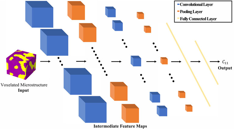
FIGURE 1. Schematic of a typical CNN architecture consisting of convolutional layers, pooling layers, and fully connected layers.

The reader is referred to various excellent texts (e.g., LeCun et al., 2015; Emmert-Streib et al., 2020; Zhang et al., 2021) for an introduction to the basics of machine learning. Here, we briefly present the primary components of the CNNs discussed in this work. A convolutional layer applies a linear transformation (performed as a convolution of a learned kernel on the input) followed by a non-linear activation applied pointwise on the feature map. The PReLU activation function defined below has been used in this work:

$\text{PReLU}\left(\text{x}\right)=\{\begin{array}{c}x, if x\ge 0\\ ax, otherwise\end{array}(2)$

A stride (Goodfellow et al., 2016; Zhang et al., 2021) can be implemented in the convolution operation to effectively coarsen the input, which helps reduce the size of the transformed feature map (this is needed as most CNNs start with high-dimensional spatial maps as input and produce low dimensional targets; see Figure 1. Pooling (Goodfellow et al., 2016; Zhang et al., 2021) is another dimensionality reduction technique that is used extensively in CNN architectures. Specifically, this work employs global average pooling where a feature map produced in an output channel is simply replaced by its average. Most CNN architectures implement fully connected layers in the last few transformation layers. Unlike the convolution layers, fully connected layers treat each input feature independently in the linear transformation. Consequently, fully connected layers dramatically increase the expressivity of the CNN models along with a concomitant increase in the number of model-fit parameters. Consequently, the fully connected layers also make the CNN models prone to over-fit.

CNNs have been successfully employed to model the microstructure-property relationships in heterogeneous (composite) material systems (Yang et al., 2018; Rao and Liu, 2020; Eidel, 2021). However, the CNN architectures designed for predicting the effective property of a microstructure have not differed significantly from the CNNs designed for machine vision problems (Lecun et al., 1998). For example, Yang et al. (2018) employed a CNN to predict the $C_{1111}$ component of the effective elastic stiffness tensor of a composite using a voxelated representation of its RVE as the input. Their CNN model contained approximately 3.2 million trainable parameters, the majority of which reside in the fully connected layers. More recently, Eidel (2021) improved the CNN model from Yang et al. (2018) by significantly reducing the number of neurons in the fully connected layers, which correspondingly reduces the number of trainable parameters. However, the CNN architecture still has approximately 2.9 million trainable parameters, of which approximately 1.8 million parameters are in the fully connected layers. Because the models are trained using relatively small datasets, typically containing only about ${10}^4$ (Yang et al., 2018; Eidel, 2021) training datapoints, the chances of the CNN model being an over-fit are significant. As already discussed, the CNN architectures used in the prior microstructure-property modeling efforts exhibit the following additional limitations: 1) the use of discrete microstructures as input makes it difficult to employ them in exploring inverse microstructure-design solutions (because of the difficulty in delineating the unimaginably large input domain), and 2) they do not automatically reflect the desired translation invariance.

3 New Protocol for Building Property Closures

This work proposes a new protocol for constructing property closures that leverages the prior advances made in both the MSD and MKS frameworks. More specifically, the proposed protocol combines the concepts of 2-point spatial correlations and their hulls developed in the MSD framework (Adams et al., 2013) with a new CNN architecture that avoids the use of fully connected layers. The proposed protocol involves two main steps: 1) building a robust surrogate model that captures the 2-point spatial correlations-property linkage of interest using the new CNN architecture, which employs a much lower number of model fit-parameters compared to current benchmarks (Yang et al., 2018; Eidel, 2021), and 2) constructing the property closure by systematically exploring the 2-point spatial correlations hull with the new CNN model. This new protocol is developed and demonstrated in this paper for constructing the property closure for selected components of the effective elastic stiffness tensor in a high-contrast composite material system.

3.1 Convolutional Neural Network Model for Microstructure-Property Linkages

The first step of the proposed protocol for building property closures is to establish a robust surrogate model that takes 2-point spatial correlations as the input and predicts the effective properties of interest. The many benefits that could come from the use of 2-point spatial correlations as the input instead of the discrete microstructure have already been discussed earlier. It is emphasized here that the features identified by the 2-point spatial correlations are expected to serve as universal features for all effective anisotropic material properties of interest (Garmestani et al., 1998; Cecen et al., 2014; Gupta et al., 2015; Kalidindi, 2015; Paulson et al., 2017; Yabansu et al., 2020; Generale and Kalidindi, 2021). Therefore, it should be possible to create microstructure-property surrogates capable of concurrently predicting multiple effective anisotropic material properties. It is further emphasized that the relationships of interest have to be necessarily formulated in the direction of microstructure → property (and not in the inverse direction) as these are expected to be many-to-one relationships. In other words, microstructures exhibiting different 2-point spatial correlations can produce the exact same effective property, because the effective property reflects a suitably averaged bulk response of the material³.

A few example RVEs and their 2-point spatial correlation maps are presented in Figure 2. It should be noted that 2-point spatial correlation maps are continuous spatial fields with a natural origin corresponding to the zero vector (i.e., $\mathit{r}=0$ in Eq. 1). Note that the 2-point spatial correlation maps exhibit a sharp peak at $\mathit{r}=0$ and generally decrease with increasing $\left|\mathit{r}\right|$. More specifically, the peak value is equal to the phase volume fraction, while the asymptotic value at large $\left|\mathit{r}\right|$ is equal to the square of the phase volume fraction. Additionally, the 2-point spatial correlations capture a number of other important details of the microstructure, including size and shape distributions (Fullwood et al., 2010; Kalidindi, 2015). Indeed, it is seen from Figure 2 that the shape of the central peak in the 2-point spatial correlations mimics the average shape of the features in the microstructure. The presence of the natural origin at $\mathit{r}=0$ imparts the desired translational invariance of the effective properties described earlier. The 2-point spatial correlations maps used as inputs to the CNNs developed in this work include vectors with x, y, and z components in the integer range $\left\{-15,\dots , 0, \dots , 15\right\}$. Although the vectors defining spatial correlations have physical units of length, they are used here with arbitrary units (these default to voxels of unit size in this work), as is typically done in FEM of composite RVEs. This is because the material constitutive law (i.e., Hooke’s law for elasticity) employed in these models does not contain any characteristic length scales. Consequently, the values of the effective stiffness of the RVE are completely independent of the physical length of each voxel in the RVE. However, one must pay attention to the voxelization itself in creating the RVEs. The use of coarser voxels will lead to inaccurate representation of the smallest features (i.e., phase regions) in the RVE, while the use of finer voxels will increase the computational cost. Prior work (Latypov et al., 2019; Marshall and Kalidindi, 2021) has utilized successfully RVEs of resolution $27 X 27 X 27$ in modelling the homogenized plastic response of composite microstructures. The resolution of the RVEs in this work was increased to $31 X 31 X 31$ to allow for a slightly improved representation of the RVEs used to capture the salient microstructure-property linkages for the present application. Further increase in the RVE resolutions was not possible for the present study because of the high computational cost involved. As a result of the considerations described above, the 2-point spatial correlation map used as input to the CNN was standardized as a 3-D array of size $31 X 31 X 31$ (with $\mathit{r}=0$ corresponding to the element (16, 16, 16) of this array). Note that the elements of this array take continuous values only in the range $\left[\mathrm{0,1}\right]$.

FIGURE 2

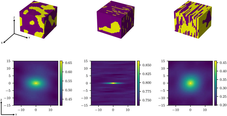
FIGURE 2. Example 3-D RVEs with the corresponding Y-Z mid-sections of their 2-point spatial correlations. It is seen that the 2-point autocorrelations capture various salient measures of the microstructures (for example, the center peak in these plots reflects the phase volume fraction and the shape of the central peak region reflects the average shape of the phase regions).

Prior work (Garmestani et al., 1998; Cecen et al., 2014; Gupta et al., 2015; Kalidindi, 2015; Paulson et al., 2017) has also shown that the 2-point spatial correlations can serve as universal features for correlating the microstructure to its many different effective (bulk) properties. The theoretical justification for this claim is most clearly seen in the statistical continuum theories formulated by Kröner (1971). Consequently, the use of 2-point spatial correlations as input can offer attractive avenues for creating high-fidelity multi-output CNN models, where each output corresponds to a different effective property of interest. In other words, one can aim to build CNN architectures that learn the common salient microstructure features that are capable of making sufficiently accurate predictions for the different effective properties of interest. Such multi-output CNNs would implicitly account for cross-correlations between the different effective properties of the RVE, making the predictions more reliable and robust. In this work, we will specifically explore multi-output CNNs for the predictions of $C_{1111} \text{and} C_{1212}$ components of the effective elastic stiffness tensor for high contrast composites.

The use of 2-point spatial correlations, instead of the voxelated microstructures, as input to the CNN essentially constitutes feature engineering. It should be recognized that most applications of CNNs do not apply any feature engineering steps. In fact, CNNs are generally touted as model building approaches that do not require feature-engineering. However, for our application, the established physics (i.e., statistical continuum mechanics theories (Kröner, 1971; Torquato, 2002)) has already proven that the 2-point spatial correlations can serve as versatile microstructural features with a number of desired characteristics described earlier. CNN models are ill-equipped to learn the 2-point spatial correlations from the discrete microstructures by themselves, because the auto-correlations and cross-correlations are not easily approximated by the various transformation layers used in the CNNs. Thus, it is likely to be much more beneficial to first compute the 2-point spatial correlations as a feature engineering step, and subsequently use them as inputs into a CNN model for predicting the effective properties. One of the main benefits anticipated would be a dramatic reduction in the number of model fit parameters. A critical evaluation of this hypothesis is one of the main goals of this work.

Towards the goals described above, we primarily focused on designing CNN architectures for our study that do not have any fully connected layers. After a few trials, we arrived at Model A (see Table 1) that showed better accuracy than the benchmarks with far fewer number of trainable parameters (discussed in more detail in the next section). We believe that this dramatic reduction of model complexity is attributable to the fact that we are using the 2-point spatial correlations as input to the CNN, in place of the voxelated microstructure. In order to validate this hypothesis, we created Model B (see Table 1), with the only difference from Model A coming from the use of the voxelated microstructure as the input to the CNN. It was also generally observed that the CNN models produced in this work needed far few layers compared to the benchmarks. This is because of the already feature-engineered inputs (i.e., 2-point spatial correlations). Furthermore, the architectures explored in this work achieved the needed dimensionality reduction in the feature maps by using stride in the first convolutional layer. A final dimensionality reduction is accomplished using global average pooling in the final layer, effectively transforming the feature maps into scalar outputs (i.e., targets). Note that the CNN architectures explored in our work are drastically simplified compared to the current benchmarks (see Table 1).

TABLE 1

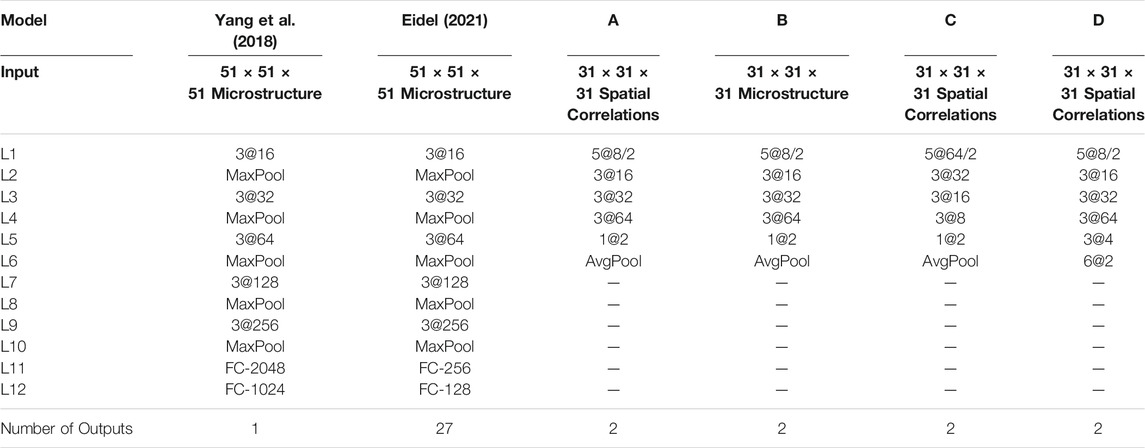
TABLE 1. Examples of different CNN architectures explored in this work along with the relevant benchmarks from literature. The notation a@b/c indicates a axaxa kernel, applied with a stride of c, and b channels. The default value of stride, when not mentioned, is one.

The architectures of Models A and B follow the current benchmarks in that they start with a relatively small number of channels in the first layer and systematically increase the number of channels in the subsequent layers. Consequently, these conventional architectures aim to initially identify a smaller number of macroscale features and then further transform them in the subsequent layers into the salient features that strongly correlate with the output. We also explored the possible benefits of inverting this architecture, i.e., starting with a large number of channels in the first layer and systematically reducing the number of channels in subsequent layers. The general idea of these inverted architectures is that they allow the initial capture of a large number of potential features, and subsequently transform them to a smaller number of salient features. Another advantage is that these inverted architectures are more naturally aligned with the dimensionality reduction needed in our application - from the higher-dimensional input to the low-dimensional output. Model C (see Table 1) shows an example of this architecture. It was also observed that the global average pooling in the last layer was essential for producing high-fidelity CNN models for our application. In an effort to critically validate this concept, we created several CNN architectures that avoided the use of the average pooling layer and accomplished the necessary dimensionality reduction exclusively through the use of convolutional layers. Model D (see Table 1) shows one such architecture, which is very similar to Model A. Note also that the change from Model A architecture to Model D architecture actually increases the number of trainable parameters and allows for richer non-linear transformations (i.e., increases model expressivity). It will be shown in the next section that this increase in model expressivity dies not necessarily result in an improvement in model fidelity. The performance of Models A through D will be discussed extensively in the next section.

The dataset employed in this work to train the CNN networks consisted of 20,480 two-phase microstructures and their corresponding FEM-estimated $C_{1111} \text{and} C_{1212}$ components of the effective elastic stiffness tensor. The details of the generation of the microstructures and the finite element models used in the estimation of the effective elastic properties have been described in prior work (Kelly and Kalidindi, 2021). The microstructures exhibited volume fractions ranging from 0 to 100%. For the two-phase microstructures studied in this work, only the $f_r^{11}$ are independent (Niezgoda et al., 2008). Consequently, only these are used as input to the CNNs. The finite element models used for the estimation of the effective properties used periodic boundary conditions (Landi et al., 2010). Specifically, the $C_{1111}$ component of the elastic stiffness tensor was estimated by imposing an average uniaxial strain of ${\overline{\text{ε}}}_{11}=0.001$ on the RVE, computing the average stress ${\overline{\sigma }}_{11}$ from the FE simulation, and dividing it by the imposed strain ($0.001$). The $C_{1212}$ component of the effective elastic stiffness tensor was similarly evaluated by imposing an average shear strain. The elastic properties of the two isotropic phases used in this study were assigned using Poisson ratios $\left({\text{ν}}_1,{\text{ν}}_2\right)$ and Young’s Moduli ($E_1,E_2)$. The following specific values were used: ${\text{ν}}_1={\text{ν}}_2=0.3$, $E_1=120$ and $E_2=\mathrm{6,000}$ (as already noted, in the FEM simulations, these are associated with arbitrary but consistent units). These selections correspond to a high contrast ratio of 50 (defined by the ratio $\frac{E_2}{E_1}$) for the composite material system studied here. Because of the linearity of the elasticity problem, the CNN model generated here can be applied to any composite material system with the same contrast value and the same values of the Poisson ratios, simply by applying a suitable scaling factor. It should be noted that although the level of contrast explored in this work is relatively high, it is still far less than the infinite contrast experienced in porous solids (for example, commonly encountered in additively manufactured components). We do believe that the microstructure design strategy proposed here is extendable to such extremely high contrast composites.

3.2 Property Closure Construction

In principle, the property closure should be constructed by mapping the complete 2-point spatial correlations space to the property space of interest. As already mentioned earlier, the protocol developed and implemented in this study aims to take full advantage of the fact that the complete space of the 2-point spatial correlations delineates a convex hull. The mapping between the 2-point spatial correlations and the effective properties of interest will be approximated by a suitable multi-output CNN model. Although the 2-point spatial correlations space is continuous and convex, it is still too large to explore using brute-force approaches. A clever strategy is therefore needed to successfully explore the complete space of 2-point spatial correlations and map it into the property space of interest. The following protocol (see Figure 3) is designed and implemented in this work:

Step 1: Create a large initial set of voxelated eigen microstructures and compute their 2-point spatial correlations. Additionally, estimate their corresponding effective properties using suitable finite element models (i.e., applying periodic boundary conditions). Build an initial estimate of the property closure using this initial dataset.

Step 2: Using a suitable algorithm (such as a convex hull algorithm), identify the boundary points of the current estimate of the property closure. This work employed the Quickhull algorithm (Barber et al., 1996), which efficiently identifies the boundary points of a convex hull defined by a set of points. These boundary points reflect extreme combinations of the properties of interest (within the current estimate of the property closure). The boundary points are updated after each iteration of the proposed protocol until the area enclosed by the boundary points does not change significantly. The microstructures corresponding to these boundary points are identified as seeds for the generation of new microstructures of interest in the next step.

Step 3: Let ${ }^a{f}_r^{11}$ and ${ }^b{f}_r^{11}$ represent the 2-point spatial correlations of two selected seeds identified in Step 2. Generate new microstructures by taking convex combinations of the 2-point spatial correlations of any selected pair of seeds from Step 2. In other words, create new microstructures as ${ }^{\ast }{f}_r^{11}= {\alpha }^a{f}_r^{11}+{\left(1-\alpha \right)}^b{f}_r^{11}$ with $0<\alpha <1$. Create as many new microstructures as needed by selecting different seeds and varying the weights of the convex combination. Ideally, one may want to focus their expansion efforts on regions of the property closure that are currently lightly populated. In other words, take convex combinations of the 2-point spatial correlations that correspond to effective property points that reside in the sparse regions of the property closure. One can also use more than two seeds at a time. As long as the weights are positive and sum to one, the generated microstructure represents convex combination of the seeds. As an example, Figure 4A depicts generation of new microstructures using three seeds, labelled as A, B, and C. All of the convex combinations are represented by points inside the triangle ABC. Microstructure D represents an example of such an interpolation. Using the CNN surrogate model, estimate the effective properties of interest for all of the new microstructures generated in this step. Add these new estimated properties to the set of points that currently approximates the property closure. Note the mapping between the microstructure space and the property space is expected to be highly non-linear, as illustrated in Figure 4B. Since a CNN provides a smooth mapping between the input and the output (Hastie et al., 2009), the triangular region ABC in the microstructure space would map to a (non-linearly) distorted but continuous triangular region with curvilinear sides in the property space.

Step 4: In this step, we will focus on extrapolations (Step 3 only used interpolations) by essentially following the same process as in Step 3, while relaxing the requirement that all weights are positive. Extrapolations are usually produced by using at least one negative weight, while requiring the weights add to one. However, we will only allow acceptable new microstructures by requiring that all values of ${ }^{\ast }{f}_r^{11}$ lie between zero and one (this condition is automatically satisfied in the interpolations in Step 3). Microstructure E in Figure 4A represents an example of the generation of a new microstructure through an extrapolation. Once again, it might be prudent to focus the generation of new microstructures in this step to the sparsely populated regions in the current estimate of the property closure.

Step 5: Validate the new microstructures added in Step 3 and 4 as needed. In particular, we note that our confidence is much higher in the 2-point spatial correlations generated as interpolations in Step 3, compared to those generated in Step 4 as extrapolations. In this work, we only validated selected new points on the expanded boundaries of the property closure. For the validation, one would have to generate a discrete microstructure corresponding to the known 2-point spatial correlations using one of the established approaches in literature (Fullwood et al., 2008b; Robertson and Kalidindi, 2021), and estimate its effective property using a suitable FEM simulation.

Step 6: Iterate Steps 2–5 as needed, while continuously adding the validated new points collected in each iteration into the current estimate of the property closure. This might necessitate re-training of the CNN model after each iteration.

FIGURE 3

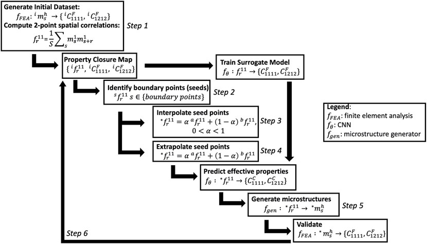
FIGURE 3. A flow chart of the proposed protocol.

FIGURE 4

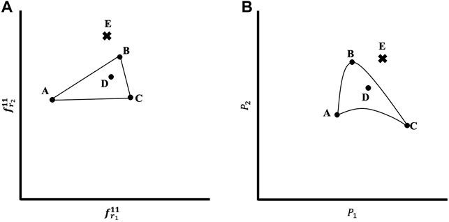
FIGURE 4. (A) Schematic illustration of the generation of new microstructures (defined in terms of 2-point spatial correlations) as interpolations or extrapolations. (B) Schematic depiction of the non-linear mapping of microstructures to the property space using a CNN model developed in this work.

The central hypotheses behind the protocol described above is that the interpolations and extrapolations of the 2-point spatial correlations can effectively explore the complete microstructure space. Moreover, since the interpolations and extrapolations are conducted using promising seeds, the protocol naturally allows targeted exploration of promising regions of the property closure. As will be shown in the next section, the CNN model facilitates a sufficiently accurate non-linear mapping of the 2-point spatial correlations into the property space.

4 Results and Discussion

The CNN architectures described in Section 3.1 were implemented in PyTorch (Paszke et al., 2019), and the property closure construction protocol described in Section 3.2 was implemented in a Python code. The set of 20, 480 data points described above was split into independent train (60%), validation (15%), and test (25%) groups. Training was conducted on a single NVIDIA V100 GPU with 16GB of memory, utilizing the Adam optimizer (Kingma and Ba, 2017) with a cosine annealing learning rate (Loshchilov and Hutter, 2017) and a training batch size of 32. The Mean Absolute Error (MAE) loss function was utilized in this work for training the CNN model. The Mean Squared Error (MSE) loss function was also explored. However, it was found that the models trained utilizing MAE produced improved learning characteristics compared to the models trained with MSE for the present application. The CNN architectures were trained for multiple epochs until the MAE loss function converged to a minimum value. Based on multiple trials, the number of epochs was fixed at 480 epochs. Using a fixed number of epochs allows for a critical comparison of the performances of the different CNN architectures explored in this work.

4.1 Development of the Convolutional Neural Network Model for Microstructure-Stiffness Linkages

As previously described, the development of a robust CNN model requires multiple trials in which the hyperparameters of the CNN architecture are systematically varied to evaluate their influence on the model fidelity. The main types of architectures explored were summarized in Table 1. The accuracy of the different CNN models produced were evaluated using the Normalized MAE (NMAE) percentage defined as

$NMAE=\frac{1}{N}{\displaystyle \sum }_{i=1}^N\left|\frac{S_i-{\widehat{S}}_i}{S_{average}}\right|\times 100(3)$

Where $S_i$ represents the ground-truth value (established here using FEM) for the output, ${\widehat{S}}_i$ represents the CNN prediction, and $S_{average}$ denotes the ensemble average of the ground-truth values from a set of $N$ observations.

Table 2 summarizes the NMAE percentages for some of the best models produced in this work, along with the corresponding values from the benchmarks reported in literature (Eidel., 2021, Yang et al., 2018). The table also summarizes the number of trainable parameters in each model as well as the sizes of the training/validation/test sizes employed in building and validating each model. As the table shows, the number of trainable parameters for each of the CNN models developed in this work is significantly smaller than those used in the current benchmarks. This is primarily because we have built our CNN models without using any fully connected layers. It is also worth noting that Eidel (2021) drastically reduced the number of neurons in the fully connected layers, when compared to Yang et al. (2018). However, even relatively smaller fully connected layers produce a very large number of trainable parameters. This is mainly because the feature maps produced at the end of the convolutional layers in the benchmark models are high-dimensional, and their reduction to a small number of features that are correlated to the outputs using the fully connected layers introduces a large number of trainable parameters. Although the Eidel (2021) model demonstrated higher accuracy than the Yang et al. (2018) model, it should be recognized that the former used significantly more training data and a much smaller test data set. As a result of these important differences between them, it is not possible to conclude conclusively that the Eidel (2021) model performance is demonstrably better than that of the Yang et al. (2018) model. However, it is clear from Table 2 that the performances of Models A, C, and D (all of which used 2-point spatial correlations as the input) are significantly better than the benchmarks, both in terms of the prediction accuracy as well the number of trainable parameters.

TABLE 2

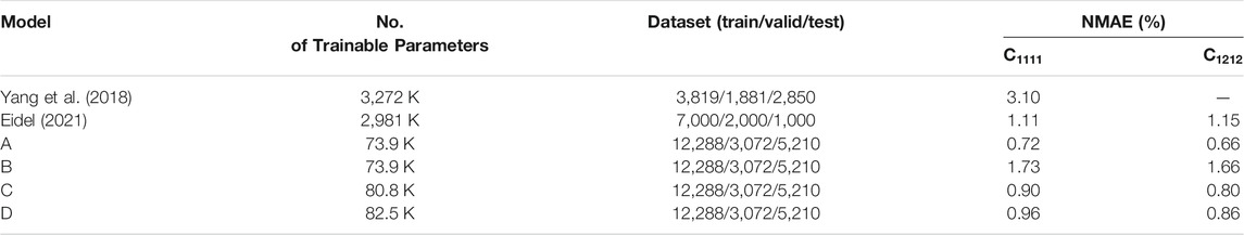
TABLE 2. Summary of the performance of selected CNN models produced in this work and their comparison with benchmarks form literature.

Comparing Models A and B, it becomes clear that changing the input to the CNN from the discrete microstructure to its 2-point spatial correlations produced a marked improvement in the model accuracy. This confirms the central hypotheses we laid out earlier. Since Model B exhibited comparable or better performance than the benchmarks (keeping in mind the larger and more diverse test sets used in this study) with a significantly smaller number of trainable parameters, it is argued that the CNN architectures without fully connected layers produce more robust models for our applications.

The improved performance of Model A over Model D underscores the need and benefits of using global average pooling as the final transformation layer for the microstructure-property CNNs. This is counter-intuitive, especially since Model D actually exhibits a higher model expressivity (i.e., it is capable of capturing more non-linear mappings). We believe the main reason for the improved performance of Model A over Model D is that the global average pooling in the last layer essentially serves as a model tree, where predictions from multiple models are averaged to produce the final prediction. Model tree strategies have been shown to improve the robustness of the surrogate models in other applications (Ho, 1995; Breiman, 2001).

Overall, it is seen that Model A outperforms all the CNN models developed to date. Most impressively, it used only 73.9 K model parameters. This is 1-2 orders of magnitude lower than the number of trainable parameters used in the current benchmarks for the same problem. As such, this model represents a significant advance in the proper use of CNNs in capturing the highly non-linear and elusive microstructure-property linkages of interest to materials design efforts. The high accuracy and robustness of the multi-output Model A can also be confirmed in the parity plots shown in Figure 5. The fact that the architecture of Model A is able to make simultaneous accurate predictions for multiple effective properties opens new research avenues for future materials design efforts.

FIGURE 5

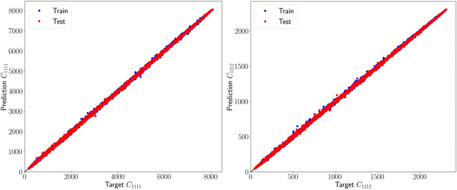
FIGURE 5. Parity plot showing the accuracy of Model A. The test points (red) are superimposed on the train points (blue). It is seen that both the train and test sets exhibit high levels of accuracy consistent with each other.

4.2 Elastic Property Closure Using Convolutional Neural Network Model

The protocol established in Section 3.2 for building property closures was implemented here using Model A. Figure 6A shows the initial estimate of the property closure using all 20,480 data points generated for training and validating the CNN model in Section 4.1. It is clear that the property closure space is not well sampled by the initial dataset. This is to be expected because the protocols used to generate the microstructures only aimed to cover as many diverse microstructures as possible. They were not in any way informed by the effective properties associated with the microstructures. Also, generating the microstructures that produce a uniform sampling of the property space are especially difficult in our application, because the input is essentially a discretized 3-D eigen microstructure.

FIGURE 6

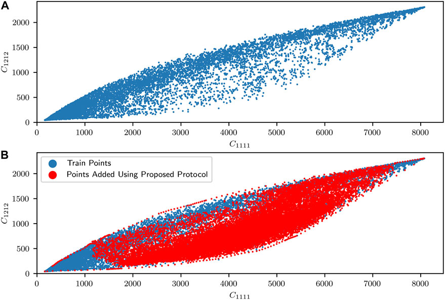
FIGURE 6. (A) Original estimate of the property closure produced using the dataset generated to initially train the CNN surrogate model. (B) Updated property closure using the protocol presented in Section 3.2. The red points represent the new points generated in the process of building the property closure.

As already described, the central advantage of the protocol described in Section 3.2 is that it allows us to generate new datapoints in selected regions of the property space. This is evident in Figure 6B, where 26,825 new datapoints (shown in red) were generated using interpolations and extrapolations in the convex hull of the 2-point spatial correlations. Note that these new datapoints were targeted to lie in specific regions of the property closure. This ability to generate new microstructures corresponding to selected regions of the property space at low computational cost is unprecedented, and is only possible because the CNN model was established using 2-point spatial correlations as the input. The central consequence of the property closure shown in Figure 6B is that it is now possible to trivially produce a large number of microstructures that correspond to any designer-specified combination of properties within the property closure.

It is emphasized here that the property closure presented in Figure 6B is the first of its kind. All previously reported property closures either used grossly simplified descriptions of the microstructure (e.g., one-point statistics) or substantially degraded models (e.g., truncated expansions, primitive bounds). As such, the property closure presented in Figure 6B represents the most accurate depiction to date of the property closure for the selected problem. Although we restricted our attention in this work to a two-phase composite with a high-contrast in the elastic properties of its constituent phases, the framework presented here is extensible to much more complicated class of composite (i.e., heterogeneous) microstructures and their different properties of interest (e.g., yield strength, conductivity, permeability).

5 Conclusion

In this work, a new CNN architecture is proposed that takes as input the 2-point spatial correlations of a voxelated eigen microstructure and predicts its effective properties of interest. Although CNNs are generally viewed as a model building technique that bypasses explicit feature engineering, it was observed that transforming the voxelated microstructure into its 2-point spatial correlations before inputting them into the CNN model dramatically improved the model accuracy and robustness. Specifically, it was shown that it is possible to build CNN models exhibiting ∼0.7% test NMAE for simultaneous predictions of two different elastic stiffness components for a high-contrast (=50) 3-D composite microstructure. This unprecedented model accuracy and robustness was made possible by avoiding the use of fully connected layers, using a global average pooling in the final layer, and using 2-point spatial correlations as input to the CNN. It was also demonstrated that the CNN model produced in this work is capable of producing the most accurate elastic property closure available today for the selected high-contrast composite material system.

Data Availability Statement

The datasets presented in this study can be found in online repositories. The names of the repository/repositories and accession number(s) can be found below: https://www.dropbox.com/sh/i9yls9d8aba2sy6/AABG-MAWABZ9gS947Phx7kgya?dl=0

Author Contributions

AM and SK conceptualized the work. AM developed the code and generated figures and tables. AM and SK wrote and edited the manuscript.

Funding

The authors acknowledge funding from NSF 2027105. This work utilized the Hive computing cluster supported by NSF 1828187 and managed by PACE at Georgia Institute of Technology, United States.

Conflict of Interest

The authors declare that the research was conducted in the absence of any commercial or financial relationships that could be construed as a potential conflict of interest.

Publisher’s Note

All claims expressed in this article are solely those of the authors and do not necessarily represent those of their affiliated organizations, or those of the publisher, the editors and the reviewers. Any product that may be evaluated in this article, or claim that may be made by its manufacturer, is not guaranteed or endorsed by the publisher.

Acknowledgments

The authors thank Conlain Kelly and Andreas Robertson for their helpful comments in guiding this work.

Footnotes

¹This term is generally used to refer to the salient details of the material internal structure which often includes statistical information on the size, shape, and placement of the different material local states (e.g., thermodynamic phases).

²This implies that if one extends the original RVE in all directions utilizing periodicity and takes a new RVE of the same size but with a different starting point, its effective property would be exactly the same as the original RVE.

³The reader is pointed to prior work on iso-property surfaces in microstructure hulls (Knezevic and Kalidindi, 2007; Fullwood et al., 2010) to visualize the many-to-one microstructure-property linkages.

References

Adams, B. L., Kalidindi, S., and Fullwood, D. T. (2013). Microstructure-sensitive Design for Performance Optimization. Waltham, MA: Butterworth-Heinemann

Google Scholar

Adams, B. L., Henrie, A., Henrie, B., Lyon, M., Kalidindi, S. R., and Garmestani, H. (2001). Microstructure-sensitive Design of a Compliant Beam. J. Mech. Phys. Sol. 49, 1639–1663. doi:10.1016/S0022-5096(01)00016-3

CrossRef Full Text | Google Scholar

Barber, C. B., Dobkin, D. P., and Huhdanpaa, H. (1996). The Quickhull Algorithm for Convex Hulls. ACM Trans. Math. Softw. 22, 469–483. doi:10.1145/235815.235821

CrossRef Full Text | Google Scholar

Bishop, C. M. (2006). Pattern Recognition and Machine Learning, Information Science and Statistics. New York: Springer.

Google Scholar

Brands, D., Balzani, D., Scheunemann, L., Schröder, J., Richter, H., and Raabe, D. (2016). Computational Modeling of Dual-phase Steels Based on Representative Three-Dimensional Microstructures Obtained from EBSD Data. Arch. Appl. Mech. 86, 575–598. doi:10.1007/s00419-015-1044-1

CrossRef Full Text | Google Scholar

Breiman, L. (2001). Random Forests. Mach. Learn. 45, 5–32. doi:10.1023/A:1010933404324

CrossRef Full Text | Google Scholar

Brough, D. B., Wheeler, D., and Kalidindi, S. R. (2017a). Materials Knowledge Systems in Python-A Data Science Framework for Accelerated Development of Hierarchical Materials. Integr. Mater. Manuf Innov. 6, 36–53. doi:10.1007/s40192-017-0089-0

PubMed Abstract | CrossRef Full Text | Google Scholar

Brough, D. B., Wheeler, D., Warren, J. A., and Kalidindi, S. R. (2017b). Microstructure-based Knowledge Systems for Capturing Process-Structure Evolution Linkages. Curr. Opin. Solid State. Mater. Sci. 21, 129–140. doi:10.1016/j.cossms.2016.05.002

CrossRef Full Text | Google Scholar

Cecen, A., Dai, H., Yabansu, Y. C., Kalidindi, S. R., and Song, L. (2018). Material Structure-Property Linkages Using Three-Dimensional Convolutional Neural Networks. Acta Materialia 146, 76–84. doi:10.1016/j.actamat.2017.11.053

CrossRef Full Text | Google Scholar

Cecen, A., Fast, T., and Kalidindi, S. R. (2016). Versatile Algorithms for the Computation of 2-point Spatial Correlations in Quantifying Material Structure. Integr. Mater. Manuf Innov. 5, 1–15. doi:10.1186/s40192-015-0044-x

CrossRef Full Text | Google Scholar

Çeçen, A., Fast, T., Kumbur, E. C., and Kalidindi, S. R. (2014). A Data-Driven Approach to Establishing Microstructure-Property Relationships in Porous Transport Layers of Polymer Electrolyte Fuel Cells. J. Power Sourc. 245, 144–153. doi:10.1016/j.jpowsour.2013.06.100

CrossRef Full Text | Google Scholar

Cybenko, G. (1989). Approximation by Superpositions of a Sigmoidal Function. Math. Control. Signal. Syst. 2, 303–314. doi:10.1007/BF02551274

CrossRef Full Text | Google Scholar

Eidel, B. (2021). Deep Convolutional Neural Networks Predict Elasticity Tensors and Their Bounds in Homogenization. Preprint. arXiv:2109.03020.

Google Scholar

Emmert-Streib, F., Yang, Z., Feng, H., Tripathi, S., and Dehmer, M. (2020). An Introductory Review of Deep Learning for Prediction Models with Big Data. Front. Artif. Intell. 3, 4. doi:10.3389/frai.2020.00004

PubMed Abstract | CrossRef Full Text | Google Scholar

Fast, T., Knezevic, M., and Kalidindi, S. R. (2008). Application of Microstructure Sensitive Design to Structural Components Produced from Hexagonal Polycrystalline Metals. Comput. Mater. Sci. 43, 374–383. doi:10.1016/j.commatsci.2007.12.002

CrossRef Full Text | Google Scholar

Fullwood, D. T., Adams, B. L., and Kalidindi, S. R. (2008a). A strong Contrast Homogenization Formulation for Multi-phase Anisotropic Materials. J. Mech. Phys. Sol. 56, 2287–2297. doi:10.1016/j.jmps.2008.01.003

CrossRef Full Text | Google Scholar

Fullwood, D. T., Adams, B. L., and Kalidindi, S. R. (2007). Generalized Pareto Front Methods Applied to Second-Order Material Property Closures. Comput. Mater. Sci. 38, 788–799. doi:10.1016/j.commatsci.2006.05.016

CrossRef Full Text | Google Scholar

Fullwood, D. T., Niezgoda, S. R., Adams, B. L., and Kalidindi, S. R. (2010). Microstructure Sensitive Design for Performance Optimization. Prog. Mater. Sci. 55, 477–562. doi:10.1016/j.pmatsci.2009.08.002

CrossRef Full Text | Google Scholar

Fullwood, D. T., Niezgoda, S. R., and Kalidindi, S. R. (2008b). Microstructure Reconstructions from 2-point Statistics Using Phase-Recovery Algorithms. Acta Materialia 56, 942–948. doi:10.1016/j.actamat.2007.10.044

CrossRef Full Text | Google Scholar

Garmestani, H., Lin, S., and Adams, B. L. (1998). Statistical Continuum Theory for Inelastic Behavior of a Two-phase Medium. Int. J. Plasticity 14, 719–731. doi:10.1016/S0749-6419(98)00019-9

CrossRef Full Text | Google Scholar

Generale, A. P., and Kalidindi, S. R. (2021). Reduced-order Models for Microstructure-Sensitive Effective thermal Conductivity of Woven Ceramic Matrix Composites with Residual Porosity. Compos. Structures 274, 114399. doi:10.1016/j.compstruct.2021.114399

CrossRef Full Text | Google Scholar

Ghosh, S., Lee, K., and Moorthy, S. (1995). Multiple Scale Analysis of Heterogeneous Elastic Structures Using Homogenization Theory and Voronoi Cell Finite Element Method. Int. J. Sol. Structures 32, 27–62. doi:10.1016/0020-7683(94)00097-G

CrossRef Full Text | Google Scholar

Goodfellow, I., Bengio, Y., and Courville, A. (2016). Deep Learning, Adaptive Computation and Machine Learning. Cambridge, Massachusetts: The MIT Press.

Google Scholar

Gupta, A., Cecen, A., Goyal, S., Singh, A. K., and Kalidindi, S. R. (2015). Structure-property Linkages Using a Data Science Approach: Application to a Non-metallic Inclusion/steel Composite System. Acta Materialia 91, 239–254. doi:10.1016/j.actamat.2015.02.045

CrossRef Full Text | Google Scholar

Hastie, T., Tibshirani, R., and Friedman, J. H. (2009). The Elements of Statistical Learning: Data Mining, Inference, and Prediction. in” Springer Series in Statistics. 2nd ed. (New York, NY: Springer)

Google Scholar

He, K., Zhang, X., Ren, S., and Sun, J. (2016). Deep Residual Learning for Image Recognition. in” 2016 IEEE Conference on Computer Vision and Pattern Recognition (CVPR). Presented at the 2016 IEEE Conference on Computer Vision and Pattern Recognition (CVPR). USA: IEEE, Las VegasNV, 770–778. doi:10.1109/CVPR.2016.90

CrossRef Full Text | Google Scholar

Jung, J., Yoon, J. I., Park, H. K., Jo, H., and Kim, H. S. (2020). Microstructure Design Using Machine Learning Generated Low Dimensional and Continuous Design Space. Materialia 11, 100690. doi:10.1016/j.mtla.2020.100690

CrossRef Full Text | Google Scholar

Kalidindi, S. R., Binci, M., Fullwood, D., and Adams, B. L. (2006). Elastic Properties Closures Using Second-Order Homogenization Theories: Case Studies in Composites of Two Isotropic Constituents. Acta Materialia 54, 3117–3126. doi:10.1016/j.actamat.2006.03.005

CrossRef Full Text | Google Scholar

Kalidindi, S. R. (2015). Hierarchical Materials Informatics: Novel Analytics for Materials Data. Amsterdam: Elsevier.

Google Scholar

Kalidindi, S. R., Niezgoda, S. R., Landi, G., Vachhani, S., and Fast, T. (2010). A Novel Framework for Building Materials Knowledge Systems. Comput. Mater. Contin. 17, 103. doi:10.3970/cmc.2010.017.103

CrossRef Full Text | Google Scholar

Kalidindi, S. R., and Schoenfeld, S. E. (2000). On the Prediction of Yield Surfaces by the crystal Plasticity Models for Fcc Polycrystals. Mater. Sci. Eng. A 293, 120–129. doi:10.1016/S0921-5093(00)01048-0

CrossRef Full Text | Google Scholar

Kelly, C., and Kalidindi, S. R. (2021). Recurrent Localization Networks Applied to the Lippmann-Schwinger Equation. Comput. Mater. Sci. 192, 110356. doi:10.1016/j.commatsci.2021.110356

CrossRef Full Text | Google Scholar

Kingma, D. P., and Ba, J. (2017). Adam: A Method for Stochastic Optimization. Preprint. arXiv:1412.6980 Cs.

Google Scholar

Knezevic, M., and Kalidindi, S. R. (2007). Fast Computation of First-Order Elastic-Plastic Closures for Polycrystalline Cubic-Orthorhombic Microstructures. Comput. Mater. Sci. 39, 643–648. doi:10.1016/j.commatsci.2006.08.025

CrossRef Full Text | Google Scholar

Knezevic, M., Kalidindi, S. R., and Mishra, R. K. (2008). Delineation of First-Order Closures for Plastic Properties Requiring Explicit Consideration of Strain Hardening and Crystallographic Texture Evolution. Int. J. Plasticity 24, 327–342. doi:10.1016/j.ijplas.2007.05.002

CrossRef Full Text | Google Scholar

Kollmann, H. T., Abueidda, D. W., Koric, S., Guleryuz, E., and Sobh, N. A. (2020). Deep Learning for Topology Optimization of 2D Metamaterials. Mater. Des. 196, 109098. doi:10.1016/j.matdes.2020.109098

CrossRef Full Text | Google Scholar

Krizhevsky, A., Sutskever, I., and Hinton, G. E. (2017). ImageNet Classification with Deep Convolutional Neural Networks. Commun. ACM 60, 84–90. doi:10.1145/3065386

CrossRef Full Text | Google Scholar

Kröner, E. (1971). Statistical Continuum Mechanics. Statistical Continuum Mechanics, CISM International Centre for Mechanical Sciences. Vienna: Springer Vienna. doi:10.1007/978-3-7091-2862-6

CrossRef Full Text | Google Scholar

Landi, G., Niezgoda, S. R., and Kalidindi, S. R. (2010). Multi-scale Modeling of Elastic Response of Three-Dimensional Voxel-Based Microstructure Datasets Using Novel DFT-Based Knowledge Systems. Acta Materialia 58, 2716–2725. doi:10.1016/j.actamat.2010.01.007

CrossRef Full Text | Google Scholar

Latypov, M. I., Toth, L. S., and Kalidindi, S. R. (2019). Materials Knowledge System for Nonlinear Composites. Comp. Methods Appl. Mech. Eng. 346, 180–196. doi:10.1016/j.cma.2018.11.034

CrossRef Full Text | Google Scholar

LeCun, Y., Bengio, Y., and Hinton, G. (2015). Deep Learning. Nature 521, 436–444. doi:10.1038/nature14539

PubMed Abstract | CrossRef Full Text | Google Scholar

Lecun, Y., Bottou, L., Bengio, Y., and Haffner, P. (1998). Gradient-based Learning Applied to Document Recognition. Proc. IEEE 86, 2278–2324. doi:10.1109/5.726791

CrossRef Full Text | Google Scholar

Loshchilov, I., and Hutter, F. (2017). SGDR: Stochastic Gradient Descent with Warm Restarts. Preprint. arXiv:1608.03983 Cs Math.

Google Scholar

Marshall, A., and Kalidindi, S. R. (2021). Autonomous Development of a Machine-Learning Model for the Plastic Response of Two-phase Composites from Micromechanical Finite Element Models. JOM 73, 2085–2095. doi:10.1007/s11837-021-04696-w

CrossRef Full Text | Google Scholar

Niezgoda, S. R., Fullwood, D. T., and Kalidindi, S. R. (2008). Delineation of the Space of 2-point Correlations in a Composite Material System. Acta Materialia 56, 5285–5292. doi:10.1016/j.actamat.2008.07.005

CrossRef Full Text | Google Scholar

Paszke, A., Gross, S., Massa, F., Lerer, A., Bradbury, J., Chanan, G., et al. (2019). PyTorch: An Imperative Style, High-Performance Deep Learning Library. Preprint. arXiv:1912.01703. Editors H. Wallach, H. Larochelle, A. Beygelzimer, F. d’ Alché-Buc, E. Fox, and R. Garnett (Curran Associates, Inc).

Google Scholar

Paulson, N. H., Priddy, M. W., McDowell, D. L., and Kalidindi, S. R. (2017). Reduced-order Structure-Property Linkages for Polycrystalline Microstructures Based on 2-point Statistics. Acta Materialia 129, 428–438. doi:10.1016/j.actamat.2017.03.009

CrossRef Full Text | Google Scholar

Pinkus, A. (1999). Approximation Theory of the MLP Model in Neural Networks. Acta Numerica 8, 143–195. doi:10.1017/S0962492900002919

CrossRef Full Text | Google Scholar

Proust, G., and Kalidindi, S. (2006). Procedures for Construction of Anisotropic Elastic-Plastic Property Closures for Face-Centered Cubic Polycrystals Using First-Order Bounding Relations. J. Mech. Phys. Sol. 54, 1744–1762. doi:10.1016/j.jmps.2006.01.010

CrossRef Full Text | Google Scholar

Rao, C., and Liu, Y. (2020). Three-dimensional Convolutional Neural Network (3D-CNN) for Heterogeneous Material Homogenization. Comput. Mater. Sci. 184, 109850. doi:10.1016/j.commatsci.2020.109850

CrossRef Full Text | Google Scholar

Robertson, A. E., and Kalidindi, S. R. (2021). Efficient Generation of Anisotropic N-Field Microstructures from 2-Point Statistics Using Multi-Output Gaussian Random Fields. SSRN J In Press. doi:10.2139/ssrn.3949516

CrossRef Full Text | Google Scholar

Roters, F., Eisenlohr, P., Hantcherli, L., Tjahjanto, D. D., Bieler, T. R., and Raabe, D. (2010). Overview of Constitutive Laws, Kinematics, Homogenization and Multiscale Methods in crystal Plasticity Finite-Element Modeling: Theory, Experiments, Applications. Acta Materialia 58, 1152–1211. doi:10.1016/j.actamat.2009.10.058

CrossRef Full Text | Google Scholar

Schmidhuber, J. (2015). Deep Learning in Neural Networks: An Overview. Neural Networks 61, 85–117. doi:10.1016/j.neunet.2014.09.003

PubMed Abstract | CrossRef Full Text | Google Scholar

Shaffer, J. B., Knezevic, M., and Kalidindi, S. R. (2010). Building Texture Evolution Networks for Deformation Processing of Polycrystalline Fcc Metals Using Spectral Approaches: Applications to Process Design for Targeted Performance. Int. J. Plasticity 26, 1183–1194. doi:10.1016/j.ijplas.2010.03.010

CrossRef Full Text | Google Scholar

Tan, R. K., Zhang, N. L., and Ye, W. (2020). A Deep Learning-Based Method for the Design of Microstructural Materials. Struct. Multidisc Optim 61, 1417–1438. doi:10.1007/s00158-019-02424-2

CrossRef Full Text | Google Scholar

Tin Kam Ho, T. K. (1995). “Random Decision Forests,” in Proceedings of 3rd International Conference on Document Analysis and Recognition. Presented at the 3rd International Conference on Document Analysis and Recognition (Montreal, Que: IEEE Comput. Soc. PressCanada), 278–282. doi:10.1109/ICDAR.1995.598994

CrossRef Full Text | Google Scholar

Torquato, S. (2002). Random Heterogeneous Materials: Microstructure and Macroscopic Properties, Interdisciplinary Applied Mathematics. New York: Springer.

Google Scholar

Wargo, E. A., Hanna, A. C., Çeçen, A., Kalidindi, S. R., and Kumbur, E. C. (2012). Selection of Representative Volume Elements for Pore-Scale Analysis of Transport in Fuel Cell Materials. J. Power Sourc. 197, 168–179. doi:10.1016/j.jpowsour.2011.09.035

CrossRef Full Text | Google Scholar

Wu, X., Proust, G., Knezevic, M., and Kalidindi, S. R. (2007). Elastic-plastic Property Closures for Hexagonal Close-Packed Polycrystalline Metals Using First-Order Bounding Theories. Acta Materialia 55, 2729–2737. doi:10.1016/j.actamat.2006.12.010

CrossRef Full Text | Google Scholar

Yabansu, Y. C., Altschuh, P., Hötzer, J., Selzer, M., Nestler, B., and Kalidindi, S. R. (2020). A Digital Workflow for Learning the Reduced-Order Structure-Property Linkages for Permeability of Porous Membranes. Acta Materialia 195, 668–680. doi:10.1016/j.actamat.2020.06.003

CrossRef Full Text | Google Scholar

Yang, Z., Yabansu, Y. C., Al-Bahrani, R., Liao, W.-k., Choudhary, A. N., Kalidindi, S. R., et al. (2018). Deep Learning Approaches for Mining Structure-Property Linkages in High Contrast Composites from Simulation Datasets. Comput. Mater. Sci. 151, 278–287. doi:10.1016/j.commatsci.2018.05.014

CrossRef Full Text | Google Scholar

Yilin, G., Fuh Ying Hsi, J., and Wen Feng, L. (2021). Multiscale Topology Optimisation with Nonparametric Microstructures Using Three-Dimensional Convolutional Neural Network (3D-CNN) Models. Virtual Phys. Prototyping 16, 306–317. doi:10.1080/17452759.2021.1913783

CrossRef Full Text | Google Scholar

Zhang, A., Lipton, Z. C., Li, M., and Smola, A. J. (2021). Dive into Deep Learning. Preprint. arXiv:2106.11342 Cs.

Google Scholar