 Philipp Rüßmann1*
 Jordi Ribas Sobreviela1,2
 Moritz Sallermann1,2,3
 Markus Hoffmann1,2
 Florian Rhiem4
 Stefan Blügel1
- 1Peter Grünberg Institut (PGI-1) and Institute for Advanced Simulation (IAS-1), Forschungszentrum Jülich, Jülich, Germany
- 2RWTH Aachen University, Aachen, Germany
- 3Science Institute and Faculty of Physical Sciences, University of Iceland, VR-III, Reykjavík, Iceland
- 4Peter Grünberg Institut/Jülich Centre for Neutron Science—Technical Services and Administration (PGI/JCNS-TA), Forschungszentrum Jülich, Jülich, Germany
Landau-Lifshitz-Gilbert (LLG) spin-dynamics calculations based on the extended Heisenberg Hamiltonian is an important tool in computational materials science involving magnetic materials. LLG simulations allow to bridge the gap from expensive quantum mechanical calculations with small unit cells to large supercells where the collective behavior of millions of spins can be studied. In this work we present the AiiDA-Spirit plugin that connects the spin-dynamics code Spirit to the AiiDA framework. AiiDA provides a Python interface that facilitates performing high-throughput calculations while automatically augmenting the calculations with metadata describing the data provenance between calculations in a directed acyclic graph. The AiiDA-Spirit interface thus provides an easy way for high-throughput spin-dynamics calculations. The interface to the AiiDA infrastructure furthermore has the advantage that input parameters for the extended Heisenberg model can be extracted from high-throughput first-principles calculations including a proper treatment of the data provenance that ensures reproducibility of the calculation results in accordance to the FAIR principles. We describe the layout of the AiiDA-Spirit plugin and demonstrate its capabilities using selected examples for LLG spin-dynamics and Monte Carlo calculations. Furthermore, the integration with first-principles calculations through AiiDA is demonstrated at the example of γ–Fe, where the complex spin-spiral ground state is investigated.
1 Introduction
Magnetic materials play an important role in modern technology. Their most important applications range from electrical motors to the storing and processing of digital information. The performance of such applications crucially relies on the performance of magnets where the knowledge of their magnetic order, the Curie temperature, the magnetic hardness or their chirality plays an important role. Computational materials design of magnetic materials and devices is a complex multi-scale problem. While quantum mechanical calculations allow to predict the interaction strength among magnetic atoms (Liechtenstein et al., 1987), large scale simulations for nanometer to micrometer length scales are unfeasible due to their computational cost. Mapping these interactions to a classical Heisenberg model allows to bridge the scales from the atomic length scale to the length scale of devices. The classical Heisenberg model is an approximation to the quantum mechanical problem which assumes that the magnetic moments are localized on atoms and can be described as classical vectors which is applicable for a wide range of materials.
Spin-dynamics calculations based on the Landau-Lifshitz-Gilbert (LLG) equation (Landau and Lifshitz, 1935; Gilbert, 2004) are a widely used tool for this multi-scale modeling of magnetic materials (Dupé et al., 2014; Hoffmann et al., 2017; Hoffmann et al., 2021; Weißenhofer et al., 2021), providing access to the collective behavior of millions of spins (Müller et al., 2019). This approach allows to find, for instance, the (non-collinear) magnetic ground state based on an energy minimization of the extended Heisenberg Hamiltonian or to study the dynamics of magnetic solitons such as skyrmions (Mühlbauer et al., 2009; Yu et al., 2010; Heinze et al., 2011; Back et al., 2020) or hopfions (Bogolubsky, 1988; Sutcliffe, 2018; Kent et al., 2021) at finite temperature. In combination with the geodesic nudged elastic band method and the harmonic transition state theory (Bessarab et al., 2012; Bessarab et al., 2015) it furthermore gives insight into the stability of aforementioned objects (Müller et al., 2019).
In this work we introduce the AiiDA-Spirit plugin that connects the Spirit code (Müller et al., 2021) to the AiiDA environment (Huber et al., 2020). AiiDA is an open-source Python framework designed around the FAIR principles of findable, accessible, interoperable and reusable data (Wilkinson et al., 2016) in computational science (Pizzi et al., 2016). Calculations that run through the AiiDA infrastructure are automatically stored as nodes in a database together with all inputs and outputs that are necessary to reproduce the simulation results. This results in an directed acyclic graph that can connect different nodes which can be used to reproduce the data provenance from a final result.
In the context of spin-dynamics simulations, a simulation result could be the magnetic ordering obtained from a minimization of the forces on each spin in an LLG calculation. The outcome of such a simulation will in general depend on input parameters such as the geometry (positions of the spins, size of simulation cell, open or periodic boundary conditions), the exchange coupling constants, or applied external fields as well as temperature noise. But also the starting point for the minimization (e.g., starting from an ordered ferromagnet or from random spin orientations) are important as local minima in the energy landscape can generally be present in which metastable states can be stabilized. To ensure reproducible calculation results, keeping track of the full data provenance of a simulation is necessary.
AiiDA’s plugin infrastructure allows to orchestrate and combine different sequences of calculations, possibly using different simulation software and methods, through a common interface. Here, we use this to first generate exchange coupling parameters from DFT calculations using the JuKKR code (The JuKKR developers, 2021) with the help of the AiiDA-KKR plugin (Rüßmann et al., 2021a; Rüßmann et al., 2021b). Then, we proceed with spin-dynamics simulations using the Spirit code (Müller et al., 2019; Müller et al., 2021) via the newly developed AiiDA-Spirit plugin (The AiiDA-Spirit developers, 2021). This allows to include the full history of the input parameter generation for spin-dynamics calculations in the provenance graph of a Spirit simulation. Using AiiDA therefore facilitates multi-scale modeling that combines the predictive power of DFT calculations and the speed and scalability of spin-dynamics simulations in the same framework.
The AiiDA engine (Uhrin et al., 2021) provides a highly scalable infrastructure that is able to deal with thousands of calculations simultaneously. Together with the simple Python interface that AiiDA-Spirit provides, spin-dynamics simulations are possible in an automated way which can be used in a high-throughput fashion. This opens new possibilities for applying the Spirit code in automated setups and as part of complex workflows in conjunction with other simulation methods such as DFT. This new capability allows to integrate Spirit in the toolbox of methods that are used in automated computational materials design for magnetic materials (Himanen et al., 2019).
This paper is structured as follows. First the methods section introduces the theory behind spin-dynamics simulations. Then the AiiDA-Spirit plugin is presented which is then applied to 1) a parameter exploration based on a toy model and a large number of high-throughput AiiDA-Spirit calculations, 2) to a simple Monte Carlo example to find the critical temperature of a model system, and 3) multi-scale modelling combining DFT and LLG calculations at the example of γ–Fe. Finally the paper concludes with a discussion of the results.
2 Methods
2.1 Spirit Theory
All spin-dynamics simulations shown throughout the paper were performed with the Spirit code (Müller et al., 2019; Müller et al., 2021). The Spirit code provides a framework for atomic-scale spin simulations and combines both a graphical user interface as well as an easy accessible Python API. All simulations performed with Spirit are based on an extended Heisenberg Hamiltonian describing the interaction of spins
Here, the first line contains the isotropic and antisymmetric exchange interactions, the later also referred to as Dzyaloshinskii-Moriya interaction. The second and third line describe the on-site anisotropy, the Zeeman energy due to an external magnetic field
A more detailed description of the Spirit framework as well as its further functionalities, such as the possibility to calculate lifetimes of magnetic textures based on the combination of geodesic nudged elastic band and harmonic transition state theory calculations, can be found in Ref. (Müller et al., 2019).
2.2 The AiiDA-Spirit Plugin
AiiDA’s plugin system allows to combine various simulation codes and methods (to date more than 60 plugins exist already (The AiiDA team, 2021)) on the same footing while augmenting the calculation done through the AiiDA infrastructure with the stored data provenance. Albeit their significance in research on magnetic materials, spin-dynamics calculations have not been at the center of the AiiDA community so far. To the best of our knowledge, besides the AiiDA-Spirit plugin presented here, only a first version of the AiiDA-UppASD plugin (Xu et al., 2021) exists for the UppASD code (Skubic et al., 2008) to combine AiiDA with a spin dynamics simulation engine.
In the context of AiiDA, a calculation plugin needs to be able to generate typical input files that are required to run a calculation through a bash script that will be generated when a calculation is submitted to a computer or as a job on a supercomputer. At the heart of the AiiDA-Spirit plugin lies the SpiritCalculation that connects the Spirit code via the Spirit Python API to AiiDA. The Layout of the SpiritCalculation is shown in Figure 1. To run a Spirit calculation a number of input nodes are required:
• a structure node describing the lattice of spins (i.e., their positions in the unit cell),
• an array of the corresponding jij_data that contains the pairwise Jij and
• the SpiritCode that is an installation of the Spirit Python API on the computer where the calculation should run,
• and run_options as well as input parameters that control the type of the Spirit run (e.g., LLG or Monte Carlo) or further settings like strength and direction of external fields, respectively.
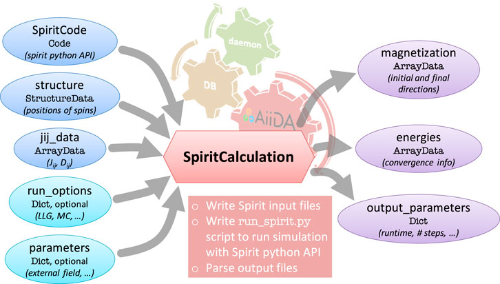
FIGURE 1. Layout of the SpiritCalculation that is at the heart of the AiiDA-Spirit plugin. On the left hand side the possible input nodes are shown which are translated by the SpiritCalculation into the appropriate input files needed to execute Spirit. The run_options and parameters input nodes are optional that default to a basic LLG calculation starting from random orientation of the spins and without external fields or temperature. The typical output nodes for a LLG calculation are shown on the right hand side.
Additionally, input modes that trigger special features of the Spirit code such as disorder and defects in the structure or pinning of spins to certain directions can be controlled with the corresponding optional input nodes. The SpiritCalculation then implements the functionality to translate this information into the appropriate input files and runs the calculation using the Spirit Python API. The AiiDA daemon automatically takes care of creating a suitable job script, copying necessary input files, and of submitting and monitoring the calculation run. Once the calculation job finishes, important output files are copied back to the retrieved folder in the AiiDA file repository associated to the AiiDA database. Then, the SpiritParser extracts useful information that should be stored in the database. For the example of a LLG calculation this entails settings such as the number of LLG steps until convergence, the used wall clock time on the computer where the calcualtion ran, an array of the energies (i.e. exchange energy per spin), and the initial and final directions of the spins in the magnetization array.
Apart from the SpiritCalculation and SpiritParser, AiiDA-Spirit comes with some tools that can be used in the typical jupyter notebook environment that is often used in the context of AiiDA. In particular we mention the show_spins tool of AiiDA-Spirit which provides the Spirit visualization capabilities in a simple Python API. This consists of a WebAssembly and WebGL version of the VFRendering library (Vfrendering, 2021) in combination with a JavaScript interface that can be used to visualize the directions of the spins from the web-browser based environment natural to jupyter notebooks.
2.3 DFT-Based Calculation of Exchange Coupling Constants
The density functional theory (DFT) results of this work were produced within the generalized gradient approximation (GGA-PBE) (Perdew et al., 1996) using the full-potential scalar-relativistic Korringa-Kohn-Rostoker Green’s function method (KKR) (Ebert et al., 2011) as implemented in the JuKKR code package (The JuKKR developers, 2021). We use an ℓmax = 3 cutoff in the angular momentum expansion with an exact description of the atomic cells (Stefanou et al., 1990; Stefanou and Zeller, 1991). After the self-consistent DFT calculations, the method of infinitesimal rotations (Liechtenstein et al., 1987) was used to compute the exchange interaction parameters Jij. The series of DFT calculations in this study are orchestrated using the AiiDA-KKR (Rüßmann et al., 2021a) plugins to the AiiDA infrastructure (Huber et al., 2020). The complete dataset that includes the full provenance of the calculations is made publicly available in the materials cloud repository (Talirz et al., 2020; Rüßmann et al., 2021).
3 Results
3.1 Automated Landau-Lifshitz-Gilbert Calculations for Model Parameter Exploration
To illustrate the usage of AiiDA-Spirit we first consider a toy model consisting of a single layer of spins in a simple-cubic lattice. The complete example is part of the dataset that accompanies this publication (Rüßmann et al., 2021). We assume only nearest neighbor interactions with isotropic exchange J1 = 10 meV and Dzyaloshinskii-Moriya interactions with a strength of D1 = 6 meV. This choice of parameters does not reflect any concrete physical system but is chosen for illustration purposes because it is known to produce skyrmions with small radii. The generation of the corresponding input node for the SpiritCalculation where including the directions of the DMI vectors can be seen in the following code snippet.
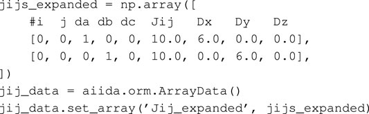
Here i, j index the lattice site in the unit cell (situated at
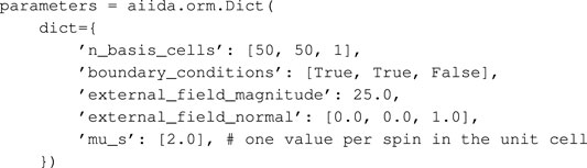
Starting from random orientations of the spins we then perform a time evolution using the LLG method with the Depondt solver (Depondt and Mertens, 2009). The parameters for the LLG calculations are summarized in Table 1.
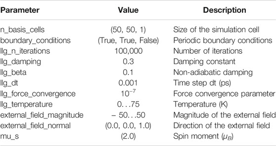
TABLE 1. Parameters for the LLG calculations of the toy model. Arrays are indicated by the square brackets. Except for external_field_magnitude and llg_temperature all parameters are kept fixed in the simulations.
To harness the high-throughput capabilities of the AiiDA-Spirit plugin we perform a series of SpiritCalculations to screen a range of external fields and temperatures. We change the temperature from 0 to 75 K in 2.5 K steps and vary the external field from − 50 T to + 50 T in steps of 2.5 T. The calculations for each parameters set are repeated 5 times starting from different random orientations of the spins for statistical averaging. This amounts to 31 × 41 × 5 = 6,355 individual SpiritCalculations that were submitted to an in-house compute cluster. We stress that the AiiDA daemon (Uhrin et al., 2021) conveniently takes care of creating submission scripts and automatically retrieves and parses the outcome of the calculations without the need for any user interaction. A visualization of the dataset and the provenance graph for this application is shown in Figure 2.
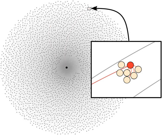
FIGURE 2. Provenance graph of the SpiritCalculations discussed in section 3.1. The graph consists of several thousand calculations that all use the same crystal structure as input (the black circle in the center) with which they are connected. The inset shows a magnified view of one of these calculations (red circle) which is connected to outgoing nodes (colored in light orange).
In order to analyze the outcome of the SpiritCalculations we chose to investigate the topological charge in the simulation cell at the end of the LLG simulation. For a continuous vector field
We added a custom post-processing step to the SpiritCalculation which uses the get_topological_charge function of the spirit Python API. This function calculates the topological charge from the discretized form of Eq. 2 as a summation over all contributions of triangles formed by neighboring spins in the simulation cell (Müller et al., 2019).
Figure 3 shows the outcome of these simulations where the topological charge is shown for all 1,271 pairs (T, Bz) together with selected spin configurations of representative calculations marked by the symbols (Figures 3B–G). The real-space spin configuration at the end of the LLG calculations were visualized using the show_spins tool of the AiiDA-Spirit plugin. It can be seen that a small external field leads to the appearance of skyrmions which in this case have a topological charge of ± 1, depending whether they form in a ferromagnetic background of spins pointing in − z (Figure 3C) or + z (Figure 3E) direction. In general, the topological charge counts the difference between the amount of skyrmions in up-domains (ρT > 0) and skyrmions in down-domains (ρT < 0) as seen for vanishing external field in (Figure 3D) where several skyrmions with opposite topological charges lead to a near cancellation of the total topological charge.
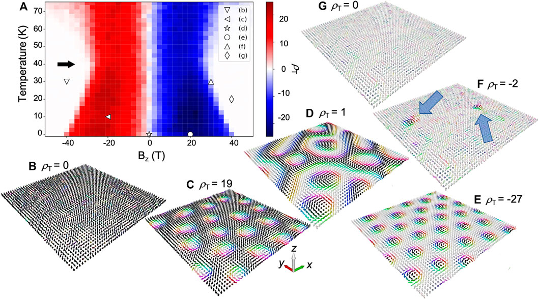
FIGURE 3. Topological charge of the toy model discussed in the text. (A) Dependence of the topological charge ρT on the external magnetic field and temperature calculated from the final spin texture after an LLG calculation. The black arrow highlights the inflection point where |ρT(Bz)| has a minimum with respect to Bz. For the parameters marked by the symbols (B–G) the resulting spin textures are shown in the corresponding panels. The arrows in (F) highlight the two skyrmions that result in a topological charge of ρT = − 2.
At very large fields, the Zeeman exchange coupling term becomes larger than the DMI energy and a homogeneous ferromagnet forms (Figures 3B,G). Temperature fluctuations tend to deform the skyrmions (Figure 3F) and destabilize them. Thus, at elevated temperatures smaller magnitudes of the external magnetic field leads to a vanishing topological charge. As highlighted by the black arrow in (Figure 3A), this is however only true up to a certain critical temperature. For T > 40 K the topological charge increases again which can be explained by the energy barrier of skyrmion formation and destruction. At these elevated temperatures the fluctuations of the spin directions are larger than 40 K ⋅ kB ≈ 3.45 meV which we conjecture is the energy barrier for skyrmion formation. While the energy barrier can in principle be calculated by performing geodesic nudged elastic band calculations, this is beyond the scope of this paper and therefore will be omitted. The larger temperature fluctuations also prohibit reaching the force convergence criterion set in the LLG calculation which means that the LLG simulation runs until the maximal simulation time of 100 ps is reached. During this simulation time, skyrmions can spontaneously form and disappear which results in a finite topological charge measured at the end of the run. In the future the real time dynamics of skyrmion creation and collapse may be the focus of the investigation. However, this approach may become unfeasible for situations where the skyrmion lifetime is very long compared to the typical time step in LLG calculations. Finally, we highlight that with increasing temperature fluctuations we also find a larger variance in the number of skyrmions when averaging over the five different starting configuration for each pair (T, Bz). This supports our interpretation that skyrmions are spontaneously created and annihilated by temperature fluctuations.
3.2 Curie Temperature Using Monte Carlo
The Monte Carlo (MC) method is a well established tool in physics which, when applied to spin systems, allows to estimate the critical temperature of the magnetic ordering (Curie temperature) (Binder and Heermann, 1997). The Spirit code (Müller et al., 2019) implements a Metropolis algorithm which can be used from AiiDA-Spirit by choosing the mc simulation method (instead of the previously used LLG method). We demonstrate the MC at the example of a simple-cubic ferromagnet with only nearest neighbor interactions J1 = 1 meV. We perform calculations for varying supercell sizes between 10 × 10 × 10 and 40 × 40 × 40 with the MC parameters given in Table 2. The results of the calculation are shown in Figure 4 where, together with the total magnetization M, the isothermal susceptibility
with
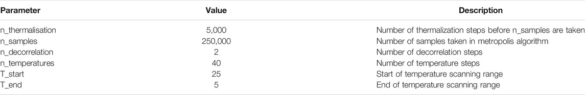
TABLE 2. Parameters for the MC calculations of the simple-cubic ferromagnet discussed in the text. Note that the chosen settings result in temperature steps of 0.5 K.
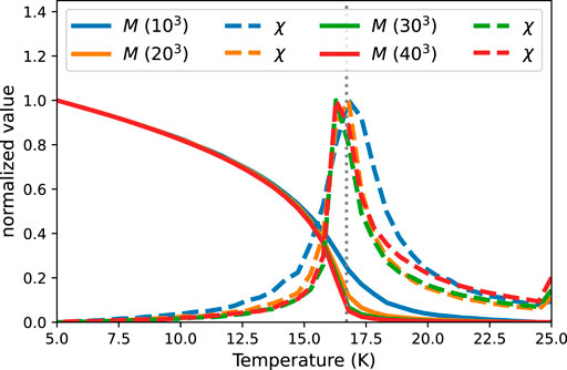
FIGURE 4. Results of the Monte Carlo calculations for a simple-cubic ferromagnetic with nearest neighbor J1 = 1 meV exchange interactions. Shown are results for 10 × 10 × 10 to 40 × 40 × 40 supercells where the solid lines show the normalized value of the total magnetization M and the dashed lines the corresponding susceptibility χ. The dashed vertical line indicate the expected value of the critical temperature at Tc = 16.71 K.
3.3 Multi-Scale Modeling: γ–Fe
We now demonstrate how the integration of the Spirit code into the AiiDA framework through the AiiDA-Spirit plugin can facilitate multi-scale modeling for magnetic materials. In this example we first calculate the exchange interaction parameters for γ–Fe using density functional theory which are then passed to the AiiDA-Spirit plugin for LLG simulations.
The γ phase of Fe is a metastable high-temperature phase where the atoms crystallize in the fcc lattice (Knöpfle et al., 2000; Sjöstedt and Nordström, 2002). This has a drastic consequence on the exchange interactions where, in contrast to the ferromagnetic bcc Fe, frustrated exchange interactions can lead to the formation of spin-spirals. Experimentally this structure of Fe can be realized in a Cu matrix (Tsunoda, 1989; Tsunoda et al., 1993). It is known that a variation of the lattice constant of γ–Fe can have drastic consequences for the magnetic ordering (Sjöstedt and Nordström, 2002). Here, we investigate bulk crystals of γ–Fe for varying lattice constants between
Figure 5 summarizes the results of the DFT calculations that were done with the AiiDA-KKR plugin (see methods section for numerical details). The total energy as a function of the lattice constant (shown in panel Figure 5A) reveals a phase transition from the low-spin state (for
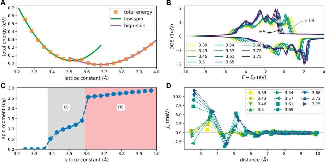
FIGURE 5. Results of the DFT calculations for γ–Fe. Total energy as a function of the lattice constant (A) where the green and violet lines show parabolic fits to low-spin
In the following, the consequences of this change for the magnetic ordering are investigated based on a series of LLG calculations using the AiiDA-Spirit plugin. In the DFT calculation we use the primitive cell which contains a single atom in the unit cell. For the spirit calculations we map the calculated exchange interactions onto the conventional unit cell consisting of four atoms. The parameters of the LLG simulations are summarized in Table 3. We study the magnetic ordering in a 40 × 40 × 40 × 4 = 256,000 spins supercell without external magnetic fields and at temperature T = 0 K. Here we focus on the ground state that forms and therefore neglect effects of temperature fluctuations and external fields which can, for example if T is high enough, overcome the energy barrier between different (metastable) magnetic orderings. We further neglect the influence of anisotropy (K⊥ = 0) in this work and we also do not include higher order exchange terms (Ki,j,k,l = 0). We choose open boundary conditions in order to not bias the eventually resulting spin-spiral wavelength by the periodicity of the supercell. Table 4 summarizes the DFT calculated values for magnetic moments and exchange coupling constants for varying lattice constants that were used in the respective SpiritCalculations. Note that the exchange coupling constants are only shown up to the seventh shell of neighbors but the calculations included pairs up to the 15th shell that are however much smaller than the values reported in Table 4.
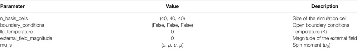
TABLE 3. Parameters for the LLG calculations for γ–Fe. Note that the simulation cell consists of 40 × 40 × 40 × 4 = 256,000 atoms due to the choice of the conventional unit cell with four atoms. The spin moment μ is extracted from the DFT calculation at the respective lattice constant and open boundary conditions are chosen. Parameters not listed here are set to the same value as in Table 1.
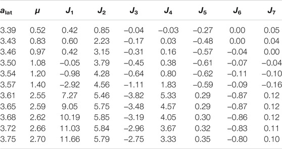
TABLE 4. Input parameters extracted from DFT that are used in the SpiritCalculations for γ–Fe for different lattice constants alat (given in Å). Listed are the magnetic moment μ (in μB per spin) and the exchange coupling parameters Jij for the first seven shells (denoted J1 to J7) which are given in meV.
We start the discussion of the LLG calculations with the results for γ–Fe in the lattice constant of Cu
with j = y, z computed with the fast Fourier transform algorithm (FFT) is shown in (Figure 6D). As expected, the FFT of the predominantly ferromagnetically ordered spins along the y-direction
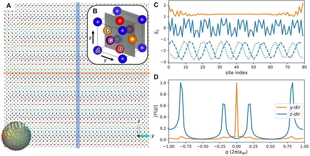
FIGURE 6. Spin-spiral ground state for γ–Fe at a lattice constant of
Figure 7 summarizes the LLG calculations for γ–Fe for varying lattice constants using the respective set of exchange parameters shown in Figure 5D. The lines in Figure 7A show the energy at the end of the LLG calculation starting either from a random spin configuration (E, dashed orange) or from the ferromagnetic (EFM, solid blue) state. We find that for lattice constants
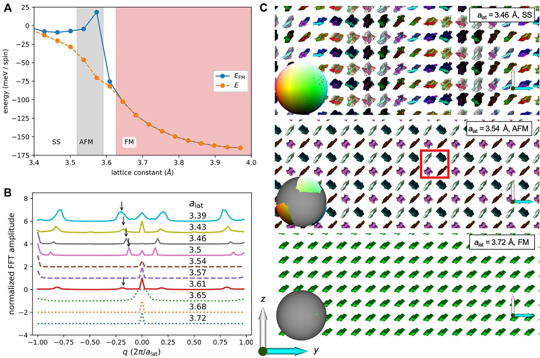
FIGURE 7. Magnetic ground state in γ–Fe from spin-dynamics simulations via the AiiDA-Spirit plugin. (A) Calculated energies per spin of the final state after an LLG calculation. Each data point uses the exchange constants computed from DFT (cf. Figure 5D). The solid blue and dashed orange lines indicate the energy computed starting from random spin configuration or the ferromagentic (FM) state. The white, grey and red shaded areas indicate if, respectively, a spin-spiral (SS), antiferromagnetic (AFM) or FM ordering is found to be the ground state. (B) Normalized Fourier transform of the z-component of the magnetization in the yz-plane for different lattice constants, shifted for clarity. Solid lines correspond to SS, dashed lines to AFM and dotted lines to FM solutions, respectively. The arrows highlight the principal wavenumber of the spin-spiral and highlight their change with the lattice constant. (C) Visualization of representative spin structures for (from top to bottom) SS, AFM and FM states where the red box in the AFM structure highlights a unit cell with the four sub-lattices. The colored points on the grey sphere in the lower left panels show a projection of the direction of the spins onto the unit sphere.
In the SS state the magnetization rotates from left to right (i.e. along the y-axis) and shows antiparallel alignment of the rows in z-direction. Along the x-axis (direction perpendicular to the drawn plane) the spins are aligned ferromagnetically, except for boundary effects at the open ends of the simulation cell (seen in the direction of the first layer of spins). In z-direction, adjacent layers are antiferromagnetically ordered. Thus the spin-spiral wavevector for these lattice constants has the form
In the AFM phase the direction of the spins separate into four sub-lattices that correspond to the four atoms in the conventional fcc unit cell. Within each sub-lattice the spins are aligned parallel and form a right angle with their neighboring spins from different sub-lattices. This is highlighted with a red box in the middle panel of (Figure 7C). In the FM phase (lower panel) all spins point in the same direction. Note that in all these calculations the spins can collectively rotate since we neglected contributions from single-ion anisotropies and do not apply an external field.
The summed magnitude of the Fourier transform along the three cardinal axes
is shown in Figure 7B for different lattice constants. Note that we have summed here over the symmetry-equivalent directions along the x- y- and z-directions because of the rotational invariance of the complete spin-structure. Starting from the smallest lattice constant of
The appearance of the AFM phase for
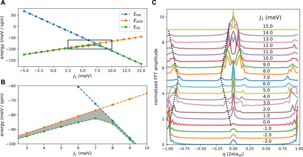
FIGURE 8. (A) Spin-spiral (SS) energies as a function of the nearest neighbor interaction J1 in comparison to ferromagnetic (FM) and antiferromagnetic (AFM) states. Exchange coupling constants were taken from the
Overall we can conclude that the resulting spin-texture in the 256,000 spin unit cell with open boundary conditions is a result of the complex competition of distance-dependent exchange couplings that favor ferromagnetic or antiferromagnetic alignments of spins or can compete and stabilize spin-spiral ground states.
4 Discussion
In this article we have presented the AiiDA-Spirit plugin that connects the spin-dynamics code Spirit to the AiiDA framework. AiiDA enables high-throughput calculations while automatically keeping track of the data provenance (Huber et al., 2020). We have demonstrated the capabilities of the AiiDA-Spirit plugin with three examples; 1) high-throughput spin-dynamics calculations based on the Landau-Lifshitz-Gilbert (LLG) equation for a toy model that shows skyrmions, 2) Monte Carlo calculations for finding the critical temperature of a simple-cubic model ferromagnet, and 3) multi-scale modelling combining density functional calculations with spin-dynamics simulations for γ–Fe.
In our high-throughput LLG calculations we performed more than 6,000 simulations of a model system consisting of a 2D lattice of spins in the simple-cubic lattice. The model parameters were chosen such that topologically nontrivial skyrmions appear in the magnetic textures. We varied the temperature and the external magnetic field as external parameters and investigate the change in the topological charge, which is a measure of the number of skyrmions that appear in the system. We find that, starting from T = 0, the transition to the homogeneous ferromagnetic phase happens at lower magnetic fields. At a certain critical temperature however the number of skyrmions starts increasing again. We interpret this as the surpassing of the energy barrier for skyrmion formation which can be overcome by temperature fluctuations of the spins. This goes hand in hand with a larger variance in the topological charge that we measure from averaging multiple runs for each pair of (T, Bz). These calculations demonstrate the possibility to employ the AiiDA-Spirit plugin for high-throughput spin-dynamics simulations which make parameter exploration easier accessible.
In our Monte Carlo calculations we showed how the complex series of calculations necessary for finding the ordering temperature of a simple-cubic ferromagnet (several calculations across the transition region from ferromagnetically ordered to paramagnetic state have to be performed) can be found from a single SpiritCalculation of the AiiDA-Spirit plugin. Our simulation result is in good agreement with the theoretically expected result. The ease-of-use for these calculations facilitate the incorporation of AiiDA-Spirit calculations in complex workflows in materials informatics for magnetic materials. Here, finding the critical temperature of a magnetic material is a very common problem.
Finally, we discussed the use case of LLG calculations for the study of the magnetic ordering of γ–Fe, which is the high-temperature fcc phase of Fe. From experiments, where Fe clusters were embedded in a Cu matrix, it is known that a spin-spiral ground state with wavevector
In contrast to the spin-spiral energy calculations of Refs. (Knöpfle et al., 2000; Sjöstedt and Nordström, 2002) we calculate the exchange parameters for the extended Heisenberg model from the method of infinitesimal rotations (Liechtenstein et al., 1987) around the collinear, ferromagnetically ordered state. These parameters are then used in the SpiritCalculations where the collective magnetic ordering is investigated in a 256,000 spin supercell. We find a strong influence of exchange interactions on the lattice constant of γ–Fe which results in a competition of ferromagnetic, antiferromagnetic and spin-spiral orderings. In our analysis of the spin-spiral wavevectors we chose to study the Fourier transform of the z-component of the spin around the three cardinal axes which are symmetry-equivalent in our approach. At the lattice constant of Cu
The change of the ordering to the antiferromagnetic state and then the reappearance of the spin-spiral state at even smaller lattice constant compared to the lattice constant of Cu on the other hand agrees well with the previously stated observation of competing magnetic orders, which are very close in energy and could coexist (Sjöstedt and Nordström, 2002). We further demonstrated the sensitivity of the magnetic ordering with a numerical experiment where we chose to modify the strength of the nearest neighbor exchange interaction J1. The resulting strong change in the spin-spiral wavevector and the magnetic ordering highlights the rich energy landscape that is underlying the complex magnetic ordering in γ–Fe.
In conclusion, we have shown how augmenting spin-dynamics calculations with the Spirit code through the AiiDA-Spirit plugin enables high-throughput spin-dynamics simulations via the AiiDA infrastructure. This was applied to model systems and, in combination with DFT calculations through the AiiDA-KKR plugin, to the multi-scale problem of the magnetic ordering in γ–Fe. Our results demonstrate that typical spin-dynamics simulations benefit from the possibility to run a large number of calculations in a high-throughput fashion. Automation of SpiritCalculations through AiiDA can be a great asset when complex model parameter spaces (i.e. external fields, temperatures, different geometries, …) are screened in order to find structure-property relations of magnetic materials. The feature of AiiDA to keep track of the data provenance is here indispensable to get reproducible results and to eventually engineer recipes for the creation and control of unconventional topological solitons in magnetic structures such as skyrmions or hopfions in the future.
Data Availability Statement
The datasets presented in this study can be found in online repositories. The names of the repository/repositories and accession number(s) can be found below: https://archive.materialscloud.org/record/2021.203 Materials Cloud Archive 2021.203 (2021). doi: 10.24435/materialscloud:9s-tx.
Author Contributions
PR and JRS programmed the first version of AiiDA-Spirit and MS and FR contributed to the further development of the plugin where FR was responsible for the spin_view functionality of AiiDA-Spirit. PR performed the DFT calculations and PR and MS performed the AiiDA-Spirit calculations. All authors discussed the results and contributed in writing the manuscript.
Funding
We acknowledge support by the Joint Lab Virtual Materials Design (JL-VMD) and thank for computing time granted by the JARA Vergabegremium (project number jara0191) and provided on the JARA Partition part of the supercomputer CLAIX at RWTH Aachen University. This work was funded by the Deutsche Forschungsgemeinschaft (DFG, German Research Foundation) under Germany’s Excellence Strategy—Cluster of Excellence Matter and Light for Quantum Computing (ML4Q) EXC 2004/1—390534769.
Conflict of Interest
The authors declare that the research was conducted in the absence of any commercial or financial relationships that could be construed as a potential conflict of interest.
Publisher’s Note
All claims expressed in this article are solely those of the authors and do not necessarily represent those of their affiliated organizations, or those of the publisher, the editors, and the reviewers. Any product that may be evaluated in this article, or claim that may be made by its manufacturer, is not guaranteed or endorsed by the publisher.
References
Back, C., Cros, V., Ebert, H., Everschor-Sitte, K., Fert, A., Garst, M., et al. (2020). The 2020 Skyrmionics Roadmap. J. Phys. D: Appl. Phys. 53, 363001. doi:10.1088/1361-6463/ab8418
Bessarab, P. F., Uzdin, V. M., and Jónsson, H. (2012). Harmonic Transition-State Theory of thermal Spin Transitions. Phys. Rev. B 85, 184409. doi:10.1103/physrevb.85.184409
Bessarab, P. F., Uzdin, V. M., and Jónsson, H. (2015). Method for Finding Mechanism and Activation Energy of Magnetic Transitions, Applied to Skyrmion and Antivortex Annihilation. Comput. Phys. Commun. 196, 335–347. doi:10.1016/j.cpc.2015.07.001
Binder, K., and Heermann, D. W. (1997). Monte Carlo Simulation in Statistical Physics. Berlin: Springer-Verlag.
Bogolubsky, I. L. (1988). Three-dimensional Topological Solitons in the Lattice Model of a Magnet with Competing Interactions. Phys. Lett. A 126, 511–514. doi:10.1016/0375-9601(88)90049-7
Depondt, P., and Mertens, F. G. (2009). Spin Dynamics Simulations of Two-Dimensional Clusters with Heisenberg and Dipole-Dipole Interactions. J. Phys. Condens. Matter 21, 336005. doi:10.1088/0953-8984/21/33/336005
Dupé, B., Hoffmann, M., Paillard, C., and Heinze, S. (2014). Tailoring Magnetic Skyrmions in Ultra-thin Transition Metal Films. Nat. Commun. 5, 4030–4036. doi:10.1038/ncomms5030
Ebert, H., Ködderitzsch, D., and Minár, J. (2011). Calculating Condensed Matter Properties Using the KKR-Green's Function Method-Recent Developments and Applications. Rep. Prog. Phys. 74, 096501. doi:10.1088/0034-4885/74/9/096501
Gilbert, T. L. (2004). Classics in Magnetics A Phenomenological Theory of Damping in Ferromagnetic Materials. IEEE Trans. Magn. 40, 3443–3449. doi:10.1109/tmag.2004.836740
Glasbrenner, J. K., Mazin, I. I., Jeschke, H. O., Hirschfeld, P. J., Fernandes, R. M., and Valentí, R. (2015). Effect of Magnetic Frustration on Nematicity and Superconductivity in Iron Chalcogenides. Nat. Phys 11, 953–958. doi:10.1038/nphys3434
Heinze, S., Von Bergmann, K., Menzel, M., Brede, J., Kubetzka, A., Wiesendanger, R., et al. (2011). Spontaneous Atomic-Scale Magnetic Skyrmion Lattice in Two Dimensions. Nat. Phys 7, 713–718. doi:10.1038/nphys2045
Himanen, L., Geurts, A., Foster, A. S., and Rinke, P. (2019). Data‐Driven Materials Science: Status, Challenges, and Perspectives. Adv. Sci. 6, 1900808. doi:10.1002/advs.201900808
Hoffmann, M., and Blügel, S. (2020). Systematic Derivation of Realistic Spin Models for Beyond-Heisenberg Solids. Phys. Rev. B 101, 024418. doi:10.1103/physrevb.101.024418
Hoffmann, M., Zimmermann, B., Müller, G. P., Schürhoff, D., Kiselev, N. S., Melcher, C., et al. (2017). Antiskyrmions Stabilized at Interfaces by Anisotropic Dzyaloshinskii-Moriya Interactions. Nat. Commun. 8, 308–309. doi:10.1038/s41467-017-00313-0
Hoffmann, M., Müller, G. P., Melcher, C., and Blügel, S. (2021). Skyrmion-antiskyrmion Racetrack Memory in Rank-One Dmi Materials. Front. Phys. 9, 668. doi:10.3389/fphy.2021.769873
Huber, S. P., Zoupanos, S., Uhrin, M., Talirz, L., Kahle, L., Häuselmann, R., et al. (2020). AiiDA 1.0, a Scalable Computational Infrastructure for Automated Reproducible Workflows and Data Provenance. Sci. Data 7, 300. doi:10.1038/s41597-020-00638-4
Kent, N., Reynolds, N., Raftrey, D., Campbell, I. T. G., Virasawmy, S., Dhuey, S., et al. (2021). Creation and Observation of Hopfions in Magnetic Multilayer Systems. Nat. Commun. 12, 1562–1567. doi:10.1038/s41467-021-21846-5
Knöpfle, K., Sandratskii, L. M., and Kübler, J. (2000). Spin Spiral Ground State of γ-Iron. Phys. Rev. B 62, 5564–5569. doi:10.1103/PhysRevB.62.5564
Krönlein, A., Schmitt, M., Hoffmann, M., Kemmer, J., Seubert, N., Vogt, M., et al. (2018). Magnetic Ground State Stabilized by Three-Site Interactions: Fe/Rh(111). Phys. Rev. Lett. 120, 207202. doi:10.1103/physrevlett.120.207202
Landau, L., and Lifshitz, E. (1935). On the Theory of the Dispersion of Magnetic Permeability in Ferromagnetic Bodies. Phys. Z. Sowjet. 851, 153.
Lebert, B. W., Gorni, T., Casula, M., Klotz, S., Baudelet, F., Ablett, J. M., et al. (2019). Epsilon Iron as a Spin-Smectic State. Proc. Natl. Acad. Sci. USA 116, 20280–20285. doi:10.1073/pnas.1904575116
Liechtenstein, A. I., Katsnelson, M. I., Antropov, V. P., and Gubanov, V. A. (1987). Local Spin Density Functional Approach to the Theory of Exchange Interactions in Ferromagnetic Metals and Alloys. J. Magnetism Magn. Mater. 67, 65–74. doi:10.1016/0304-8853(87)90721-9
Müller, G. P., Sallermann, M., Mavros, S., Rhiem, F., Schürhoff, D., Meyer, I., et al. (2021). Spirit: Spin Simulation Software. Available at: https://github.com/spirit-code/spirit (Accessed November 25, 2021).
Müller, G. P., Hoffmann, M., Dißelkamp, C., Schürhoff, D., Mavros, S., Sallermann, M., et al. (2019). Spirit : Multifunctional Framework for Atomistic Spin Simulations. Phys. Rev. B 99, 224414. doi:10.1103/PhysRevB.99.224414
Mühlbauer, S., Binz, B., Jonietz, F., Pfleiderer, C., Rosch, A., Neubauer, A., et al. (2009). Skyrmion Lattice in a Chiral Magnet. Science 323, 915–919. doi:10.1126/science.1166767
Perdew, J. P., Burke, K., and Ernzerhof, M. (1996). Generalized Gradient Approximation Made Simple. Phys. Rev. Lett. 77, 3865–3868. doi:10.1103/PhysRevLett.77.3865
Pizzi, G., Cepellotti, A., Sabatini, R., Marzari, N., and Kozinsky, B. (2016). AiiDA: Automated Interactive Infrastructure and Database for Computational Science. Comput. Mater. Sci. 111, 218–230. doi:10.1016/j.commatsci.2015.09.013
Rüßmann, P., Bertoldo, F., Bröder, J., Wasmer, J., Mozumder, R., Chico, J., et al. (2021). JuDFTteam/aiida-kkr: AiiDA Plugin for the JuKKR Codes. doi:10.5281/zenodo.3628251
Rüßmann, P., Bertoldo, F., and Blügel, S. (2021). The AiiDA-KKR Plugin and its Application to High-Throughput Impurity Embedding into a Topological Insulator. Npj Comput. Mater. 7, 13. doi:10.1038/s41524-020-00482-5
Rüßmann, P., Ribas Sobreviela, J., Sallermann, M., Hoffmann, M., Rhiem, F., and Blügel, S. (2021b). The AiiDA-Spirit Plugin for Automated Spin-Dynamics Simulations and Multi-Scale Modelling Based on First-Principles Calculations. Mater. Cloud Archive, 203. doi:10.24435/materialscloud:9s-tx
Sjöstedt, E., and Nordström, L. (2002). Noncollinear Full-Potential Studies of γ−Fe. Phys. Rev. B 66, 014447. doi:10.1103/PhysRevB.66.014447
Skubic, B., Hellsvik, J., Nordström, L., and Eriksson, O. (2008). A Method for Atomistic Spin Dynamics Simulations: Implementation and Examples. J. Phys. Condens. Matter 20, 315203. doi:10.1088/0953-8984/20/31/315203
Stefanou, N., Akai, H., and Zeller, R. (1990). An Efficient Numerical Method to Calculate Shape Truncation Functions for Wigner-Seitz Atomic Polyhedra. Comput. Phys. Commun. 60, 231–238. doi:10.1016/0010-4655(90)90009-P
Stefanou, N., and Zeller, R. (1991). Calculation of Shape-Truncation Functions for Voronoi Polyhedra. J. Phys. Condens. Matter 3, 7599–7606. doi:10.1088/0953-8984/3/39/006
Sutcliffe, P. (2018). Hopfions in Chiral Magnets. J. Phys. A: Math. Theor. 51, 375401. doi:10.1088/1751-8121/aad521
Szilva, A., Costa, M., Bergman, A., Szunyogh, L., Nordström, L., and Eriksson, O. (2013). Interatomic Exchange Interactions for Finite-Temperature Magnetism and Nonequilibrium Spin Dynamics. Phys. Rev. Lett. 111, 127204. doi:10.1103/physrevlett.111.127204
Talirz, L., Kumbhar, S., Passaro, E., Yakutovich, A. V., Granata, V., Gargiulo, F., et al. (2020). Materials Cloud, a Platform for Open Computational Science. Sci. Data 7, 299. doi:10.1038/s41597-020-00637-5
The AiiDA-Spirit developers (2021). The Aiida-Spirit Plugin. Available at: https://github.com/JuDFTteam/aiida-spirit (Accessed November 25, 2021)
The AiiDA team, (2021). AiiDA Plugin Registry. Available at: https://aiidateam.github.io/aiida-registry/ (Accessed November 25, 2021).
The JuKKR developers, (2021). The Jülich KKR Codes. Available at: https://jukkr.fz-juelich.de (Accessed November 25, 2021).
Tsunoda, Y., Nishioka, Y., and Nicklow, R. M. (1993). Spin Fluctuations in Small γ-Fe Precipitates. J. Magnetism Magn. Mater. 128, 133–137. doi:10.1016/0304-8853(93)90867-2
Tsunoda, Y. (1989). Spin-density Wave in Cubic γ-Fe and γFe100-xCox precipitates in Cu. J. Phys. Condens. Matter 1, 10427–10438. doi:10.1088/0953-8984/1/51/015
Uhrin, M., Huber, S. P., Yu, J., Marzari, N., and Pizzi, G. (2021). Workflows in AiiDA: Engineering a High-Throughput, Event-Based Engine for Robust and Modular Computational Workflows. Comput. Mater. Sci. 187, 110086. doi:10.1016/j.commatsci.2020.110086
Vfrendering, (2021). A Vector Field Rendering Library. Available at: https://github.com/FlorianRhiem/VFRendering (Accessed November 25, 2021).
Weißenhofer, M., Rózsa, L., and Nowak, U. (2021). Skyrmion Dynamics at Finite Temperatures: Beyond Thiele's Equation. Phys. Rev. Lett. 127, 047203. doi:10.1103/PhysRevLett.127.047203
Wilkinson, M. D., Dumontier, M., Aalbersberg, I. J., Appleton, G., Axton, M., Baak, A., et al. (2016). The FAIR Guiding Principles for Scientific Data Management and Stewardship. Sci. Data 3, 160018. doi:10.1038/sdata.2016.18
Xu, Q., Bergman, A., Delin, A., and Chico, J. (2021). The UppASD-AiiDA Plugin. Available at: https://github.com/UppASD/aiida-uppasd (Accessed November 25, 2021).
Keywords: spin-dynamics simulation, high-throughput computation, Landau-Lifshitz-Gilbert equation, Monte-Carlo simulation, spin-spiral state, gamma-Fe, skyrmion, antiskyrmion
Citation: Rüßmann P, Ribas Sobreviela J, Sallermann M, Hoffmann M, Rhiem F and Blügel S (2022) The AiiDA-Spirit Plugin for Automated Spin-Dynamics Simulations and Multi-Scale Modeling Based on First-Principles Calculations. Front. Mater. 9:825043. doi: 10.3389/fmats.2022.825043
Received: 29 November 2021; Accepted: 21 January 2022;
Published: 22 February 2022.
Edited by:
Simone Taioli, European Centre for Theoretical Studies in Nuclear Physics and Related Areas (ECT∗), ItalyReviewed by:
Tommaso Morresi, UMR7590 Institut de Minéralogie, de Physique des Matériaux et de Cosmochimie (IMPMC), FranceMichele Casula, Université Pierre et Marie Curie, France
Copyright © 2022 Rüßmann, Ribas Sobreviela, Sallermann, Hoffmann, Rhiem and Blügel. This is an open-access article distributed under the terms of the Creative Commons Attribution License (CC BY). The use, distribution or reproduction in other forums is permitted, provided the original author(s) and the copyright owner(s) are credited and that the original publication in this journal is cited, in accordance with accepted academic practice. No use, distribution or reproduction is permitted which does not comply with these terms.
*Correspondence: Philipp Rüßmann, cC5ydWVzc21hbm5AZnotanVlbGljaC5kZQ==