Machine Learning Assisted Design of Experiments for Solid State Electrolyte Lithium Aluminum Titanium Phosphate

Lithium-ion batteries with solid electrolytes offer safety, higher energy density and higher long-term performance, which are promising alternatives to conventional liquid electrolyte batteries. Lithium aluminum titanium phosphate (LATP) is one potential solid electrolyte candidate due to its high Li-ion conductivity. To evaluate its performance, influences of the experimental factors on the materials design need to be investigated systematically. In this work, a materials design strategy based on machine learning (ML) is employed to design experimental conditions for the synthesis of LATP. In the variation of parameters, we focus on the tolerance against the possible deviations in the concentration of the precursors, as well as the influence of sintering temperature and holding time. Specifically, models built with different design selection strategies are compared based on the training data assembled from previous laboratory experiments. The best one is then chosen to design new experiment parameters, followed by measuring the corresponding properties of the newly synthesized samples. A previously unknown sample with ionic conductivity of 1.09 × 10⁻³ S cm⁻¹ is discovered within several iterations. In order to further understand the mechanisms governing the high ionic conductivity of these samples, the resulting phase compositions and crystal structures are studied with X-ray diffraction, while the microstructures of sintered pellets are investigated by scanning electron microscopy. Our studies demonstrate the advantages of applying machine learning in designing experimental conditions by the synthesis of desired materials, which can effectively help researchers to reduce the number of required experiments.

1 Introduction

Energy is one of the core issues to be solved in the development of human society. Currently, lithium ion batteries (LIBs) are widely used, as they show great promise as an effective energy storage technology for a wide range of applications from mobile devices to electric vehicles. However, commercial LIBs confront hidden risks which are due to the utilization of fluid electrolytes, which may cause a variety of safety and performance problems, such as the potential ignition of the flammable solvent. To address these problems, lithium-ion batteries with solid electrolytes have potentials to be safer and longer-lasting alternatives with higher energy density compared to conventional liquid electrolyte batteries by allowing the use of high-voltage cathodes, which can decrease flammability, and suppress dendrite formation (Goodenough and Kim, 2010). However, the principal design challenge of solid electrolytes is their restricted ionic conductivity, which is typically many orders of magnitude lower than that of liquids (10⁻² S cm⁻¹) (Aravindan et al., 2011). The feasibility of these concepts depends on the applied solid-state electrolyte, for which a wide range of materials is being considered (Manthiram et al., 2017). One of the promising materials is the family of lithium containing NASICON (sodium super ionic conductor) materials, such as lithium aluminum titanium phosphate (LATP, Li_1+xAl_xTi_2-x(PO₄)₃), one of the most often investigated materials (Aono et al., 1990). They have received wide attention as they have emerged as particularly promising solid electrolyte candidates due to their high ionic conductivity, low cost, and stability (Rossbach et al., 2018).

The ionic conductivity of LATP is particularly high for the composition Li_1.3Al_0.3Ti_1.7(PO₄)₃, and several studies have reported values up to 10⁻³ S cm⁻¹ (Narváez-Semanate and Rodrigues, 2010; Pérez-Estébanez et al., 2014; Bucharsky et al., 2015; Ma et al., 2016). Li_1.3Al_0.3Ti_1.7(PO₄)₃ ceramics have been successfully synthesized by different routes, such as calcination of stoichiometric mixtures of oxide precursors (Arbi et al., 2002), by glass crystallization (Narváez-Semanate and Rodrigues, 2010), or by sol-gel (Bucharsky et al., 2015). However, these studies are usually limited to laboratory scale, i.e., in small quantities and under experimental environments. In order to make ceramic electrolytes usable and competitive in the next generation of batteries, it is necessary to identify processing routes for the upscale production. The sol-gel route has already been adopted successfully for the mass production of many materials for industry and therefore provides a good basis for LATP synthesis. For the sake of quality maintenance and reproducibility, the crucial processing parameters have to be identified. As the first step towards the upscaling of LATP production via the sol-gel route, influence of possible deviations in the concentration of the precursors was investigated in our previous study (Schiffmann et al., 2021). This applies especially to phosphoric acid which is difficult to specify due to its hygroscopicity. In the case when precursors are not exactly stoichiometric, this can easily lead to the second-phase formation. In particular, for LATP, such second phases have a great influence on the densification and the ionic conductivity. Hupfer et al. (2017) report how the second phases AlPO₄ and LiTiOPO₄ can have impacts on the properties of LATP. In this work, synthesis of LATP is studied by varying concentration of the reactants, dwell time, and sintering temperature while microstructures, phase compositions, and ionic conductivities of the samples are further analyzed.

A key challenge in developing better materials is the large potential search space for the optimal chemistries and processing conditions. Traditionally, the development of new materials requires a vast number of experiments guided by intuition, trial and error, and is complemented by simulations and other tools to analyze the mechanism or optimize the design (Wang et al., 2015). As a result, this process is time-consuming, challenging and is often accompanied by detours or serendipity. Recently, the use of machine learning methods to accelerate materials development has received a lot of attention and many advances using this kind of technique have been made in the study of solid-state electrolytes, such as screening fast ion conductor candidates in supervised (Sendek et al., 2017) or unsupervised (Zhang et al., 2019) manner, filtering electrolytes in consideration of suppression of dendrite formation in lithium metal anodes (Ahmad et al., 2018), and developing good candidates combining theoretical calculations as well as experimental data sets (Fujimura et al., 2013).

Among the many approaches, accelerating the research of novel materials through automated experiments (Alberi et al., 2018; Häse et al., 2019; Stein and Gregoire, 2019) instructed by artificial intelligence (AI) (Tran and Ulissi, 2018) has recently attracted a lot of interest. In particular, AI sampling algorithms (Coley et al., 2020) hold great promise for resource-constrained tasks such as materials research, since they can reduce the number of experiments required to achieve a desired property (Vasudevan et al., 2019). Among them, the Bayesian decision-theoretic approach naturally lends itself to adaptive sampling and active learning (Cohn et al., 1996). Hence, a series of active learning methods based on Bayesian optimization can be used to find the optimal material composition or to optimize the experimental parameters. This type of method has been successfully applied in different materials system, such as low thermal hysteresis shape memory alloys (Xue et al., 2016), BaTiO₃-based ceramics with better dielectric energy storage density (Yuan et al., 2019), fast ion conductors for rechargeable batteries (Jalem et al., 2018; Harada et al., 2020; Homma et al., 2020; Yang et al., 2020), oxygen evolution reaction catalyst (Rohr et al., 2020), and organic thin films (MacLeod et al., 2020).

In this work, we use a Gaussian process (GP) based Bayesian optimization (Ki Williams, 2006) to optimize the synthesis of a popular electrolyte material for solid-state lithium-ion batteries, LATP (Li_1.3Al_0.3Ti_1.7(PO₄)₃). Via the sol-gel route, it is possible to prepare the material at laboratory scale with high purity and with a maximum Li-ion conductivity in the order of 1 × 10⁻³ S cm⁻¹ at room temperature. However, for a potential commercial usage, battery-cell upscaling of the synthesis is required. Based on our previous study (Schiffmann et al., 2021), we further explore the effects of deviations in the concentration of the precursors H₃PO₄, sintering temperature and holding time on the conductivity of the synthesized electrolytes. We use machine learning methods to guide us to reduce the number of required experiments as much as possible to produce LATP with higher ionic conductivity. We train the initial model using the data points from previous experiments (sampled from an equidistant grid and this is noted as grid search) and predict the next optimal experimental configurations. The results show that newly synthesized samples guided by the model can achieve a good performance with the maximum ionic conductivity of 1.09 × 10⁻³ S cm⁻¹, in the same order of magnitude of the maximum Li-ion conductivity which LATP can achieve. This method can help to quickly narrow down the search space and assist the experimentalists in designing and analyzing experiments.

2 Experiments and Machine Learning Methods

2.1 Experiments

In our experiments, LATP powders are prepared following a modified sol-gel synthesis route described by (Bucharsky et al., 2015). Appropriate amounts of lithium acetate Li(C₂H₃O₂) ⋅2H₂O (purity $\ge 99\%$, Alfa Aesar GmbH & Co KG, Germany), aluminum nitrate Al(NO₃)₃ ⋅9H₂O (purity $\ge 98.5\%$, Merck KGaA, Germany), titanium-isopropoxide Ti[OCH(CH₃)₂]₄ (purity $\ge 98\%$, Merck KGaA, Germany) are used as precursors. Lithium acetate and aluminum nitrate are dissolved in distilled water under constant stirring. Titanium-Isopropoxide is then added dropwise to the solution. By adding the phosphoric acid slowly through a drip funnel, a white gel forms, which is then dried at room temperature for 24 h. The subsequent heat treatment is performed in two steps: first, samples are heat treated at 400°C for 6 h to achieve the precursor formation and to eliminate reaction gases; second, samples are then processed at 900°C for 8 h to complete the reaction to crystalline LATP. One sol-gel batch is prepared with all precursors in stoichiometric quantities (marked as 0.0 wt%). To test whether the sol-gel route is tolerant against possible deviations in the concentration of the precursors, we also explore different sol-gel batches with either an excess up to +7.5 wt%, or a deficiency up to −15.0 wt% of phosphoric acid compared to the stoichiometric composition.

To ensure a high sinterability, the obtained powders are further processed in a planetary ball mill. The pellets are formed by uniaxial pressing and then further densified by cold isostatic pressing at 400 MPa. All pressed samples have a green density of approximately 62% relative density. Samples are sintered at temperatures ranging from 850 to 1,050°C and isothermal sintering time between 30 and 540 min. After sintering, samples are cooled down to room temperature in furnace and their corresponding densities are determined by Archimedes’ method. For the ionic conductivity measurements, impedance analysis is performed at room temperature over the frequency range from 0.1 Hz to 1 MHz with an AC amplitude of 50 mV in the frequency response analyzer (AMTEK GmbH, VersaSTAT 4, Pennsylvania, United States). For further details of the experimental part please refer to our previous work (Schiffmann et al., 2021).

To apply machine learning methods in guiding the experimental study, 80 initial data points from the aforementioned phosphoric acid deviation study are used to train the Gaussian process regression based Bayesian optimization (GPR-BO) model. These data points are sampled from an equidistant grid from −22.5 wt% to +7.5 wt% deviation of phosphoric acid compared to the stoichiometric composition. Sintering parameters with temperatures ranging from 800°C up to 1,100°C in steps of 100°C and isothermal durations of 10, 30, 60 and 480 min are applied. To further investigate the effect of these synthesis and sintering conditions on the properties of LATP, the machine learning model is used to predict promising candidate to investigate. Considering the long time needed to synthesize samples with different acid concentrations, we expand the experimental conditions available to the model in two steps: for the first two iterations (1–2), we only allow the model to make a choice among the available samples; for the last two iterations (3–4), we expand the selection range of acid concentrations. Such kind of condition setting is derived from the results of our previous grid search study and offers an efficient compromise that would address the otherwise excessively large search space. In total, we have synthesized 22 new samples in 4 iterations following the model’s predictions. Detailed settings for the experiments are listed in Table 1.

TABLE 1

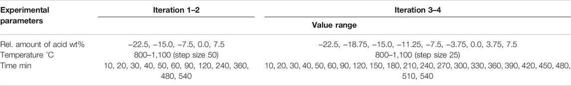
TABLE 1. Range of experimental parameters for selection.

2.2 Machine Learning Methods

2.2.1 Design Loop

Our method of applying Bayesian optimization (BO) in guiding experiments is schematically illustrated in Figure 1. The whole process is mapped as a workflow containing an iterative loop with feedback steps and it is also collectively referred to as “adaptive design.” First, the model fits the initial data points. Then the next candidate configuration is predicted and the accompanying experiment and measurements are performed. Finally, the resulting new data point is fed back into the data set for the next iteration. Key ingredients of this process for our problem are as follows: 1) collecting the training data set of the solid state electrolyte LATP, where samples are described by features, here: experimental conditions and their measured properties of interest (e.g., ionic conductivity); 2) training an inference model (Gaussian process regressor) to learn to map the input-output relationship with associated uncertainties. Then, the trained model predicts the outputs (i.e., ionic conductivities) along with their corresponding uncertainties for the whole search space; 3) choosing the combination of experimental parameters, which is expected to produce the material with better characteristics (e.g., higher ionic conductivity) by balancing the trade-off between exploitation and exploration, that is, taking both prediction (of the best known so far) and uncertainty into consideration; 4) performing experiments and measuring the corresponding properties; 5) adding the new sample to the training data set, which allows the subsequent iterative improvement of the inference model. This loop continues until performance (e.g., we have synthesized a sample with a satisfying performance) or a break condition, such as a maximum number of iterations, is met. In this work, the research data infrastructure Kadi4Mat (Brandt et al., 2021) is used to share and manage data for continuously updating the machine learning model. Besides, the whole workflow will also be integrated into this platform and serves as a demonstration for data-driven and machine learning based optimization of solid state electrolyte.

FIGURE 1

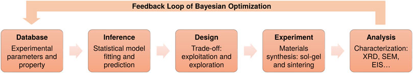
FIGURE 1. An overview of the Bayesian optimization workflow. It consists of five main components and forms an iterative loop: (i) collecting some initial data points (input-output pairs) from experiments and aggregating them into a database which will be used for training the machine learning model; (ii) fitting an inference model (e.g., a Gaussian process regression model); based on the existing data set; (iii) predicting the property in the search space along with uncertainty, taking both prediction (of the best known so far) and uncertainty (i.e., exploitation vs. exploration) into consideration for selecting the next optimal experimental configuration which has the potential to yield a better property; (iv) performing the experiment to synthesize new sample and (v) validating the new sample’s performance using different characterization techniques. The resulting sample is fed back into the initial training data set for the next iteration.

2.2.2 Bayesian Optimization

Bayesian optimization (BO) is a class of machine-learning-based optimization methods focusing on solving the problem arg max_x∈χ f(x) within a domain $\chi \subset {\mathbb{R}}^d$ as the bounding box. Its ability to optimize expensive black-box derivative-free functions makes BO extremely versatile (Shahriari et al., 2015). Recently, it has become extremely popular for tuning hyper-parameters in machine learning algorithms, especially deep neural networks (Snoek et al., 2012). A typical Bayesian optimization algorithm involves two primary components: a method for statistical inference, typically Gaussian process (GP) (Rasmussen, 2003; Williams and Rasmussen, 2006); and an acquisition function that decides where to sample. For the latter, there are many options such as PI [probability of improvement (Kushner, 1964)], EI [expected improvement (Močkus, 1975; Jones et al., 1998)] or UCB [upper confidence boundary (Auer et al., 2002)]. GP (Gaussian process) is a widely used surrogate for modeling objective functions in Bayesian optimization. The function f is typically assumed to be a GP which is determined by a mean function μ and a covariance kernel K, f ∼ $\mathcal{G}\mathcal{P}(\mu ,K)$. Given the observed data set D, the question would be where the next point to observe the function is. The meta-approach in Bayesian optimization is to design an acquisition function a(x). The acquisition function is usually an inexpensive function, which defines a balance between exploring new areas in the objective space and exploiting areas that are already known to have favorable values (Frazier, 2018). This strategy is important for helping to find the global optimum efficiently instead of being trapped in a local optimum. In short, by adopting this method, the original optimization problem is replaced with another optimization problem based on a much-cheaper function a(x).

PI is one of the earliest acquisition functions designed for Bayesian optimization which suggests maximizing the probability of improvement over the current best observed value f(x⁺), where $x^{+}={\arg \max }_{x\in D_{1:t}}f(x)$ with the observed data set D_1:t, so that

$x_{t+1}=\underset{x\in \chi }{\arg \max }{a}_{PI}\left(x\right)=\underset{x\in \chi }{\arg \max }P\left(f\left(x\right)\ge f\left(x^{+}\right)\right)=\underset{x\in \chi }{\arg \max }\mathrm{\Phi }\left(\frac{{\mu }_t\left(x;D_{1:t}\right)-f\left(x^{+}\right)}{{\sigma }_t\left(x;D_{1:t}\right)}\right)$

where Φ(⋅) is the normal cumulative distribution function, μ_t and σ_t are the posterior mean and posterior standard deviation at iteration t.

Alternatively, maximizing the expected improvement (EI) over the current best value can also be chosen, which accounts for the size of the improvement (while PI does not). It can be computed analytically as:

$x_{t+1}=\underset{x\in \chi }{\arg \max }{a}_{EI}\left(x\right)=\underset{x\in \chi }{\arg \max }\left[\left({\mu }_t\left(x;D_{1:t}\right)-f\left(x^{+}\right)\right)\mathrm{\Phi }\left(Z\right)+{\sigma }_t\left(x;D_{1:t}\right)\varphi \left(Z\right)\right]$

$Z=\frac{{\mu }_t\left(x;D_{1:t}\right)-f\left(x^{+}\right)}{{\sigma }_t\left(x;D_{1:t}\right)}$

where Φ(⋅) and ϕ(⋅) are the cumulative distribution function (CDF) and probability density function (PDF) of the standard normal distribution, respectively.

The acquisition function of UCB takes the form:

$x_{t+1}=\underset{x\in \chi }{\arg \max }{a}_{UCB}\left(x\right)=\underset{x\in \chi }{\arg \max }\left[{\mu }_t\left(x;D_{1:t}\right)+\kappa {\sigma }_t\left(x;D_{1:t}\right)\right].$

This function can be intuitively interpreted as a weighted sum of prediction of f(x) and its uncertainty. κ is a tunable hyper-parameter (usually set to be 1.96 as it represents the 95% confidence interval and generally has good performance) which controls how much of the variance in the predicted values should be taken into account. Higher value favours the exploration over exploitation and vice versa.

To predict optimal experimental parameters in an effective way, the search strategy also needs to follow the aforementioned principle, i.e., combining exploration and exploitation. The model should not only focus on the local region where the known maximum value is located, but also explore the whole search space wisely. Here, we adopt one of the widely used Bayesian optimization methods named GP-UCB [Gaussian Process Upper Confidence Boundary (Srinivas et al., 2009)], which is an intuitive algorithm inspired by the multi-armed bandit problem. We show how the GP-UCB method can be used for materials discovery, as this allows us to choose potential candidates which aims at maximizing the target property of the material. A schematic diagram of the working principle is illustrated in Figure 2. This figure shows the fitting of model with the H₃PO₄ acid at stoichiometry (namely, .0 wt%), where the x-axis stands for dwell time and the y-axis represents the sintering temperature. Larger values of the ionic conductivity are marked with brighter color. The left diagram shows what the prediction (inference) based on known data points from the grid search study looks like in the search space and the right diagram illustrates the prediction with uncertainty. It can be clearly seen that when taking the uncertainty into account, the search surface becomes significantly rugged and the location of the possible optimal value has shifted. The model will select regions worth exploring according to both the prediction and the degree of uncertainty.

FIGURE 2

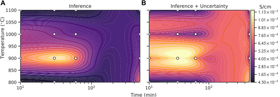
FIGURE 2. Illustration of the prediction (A) based on known data points (white points) and prediction with uncertainty (B) from the Gaussian process regression with UCB model in the search space. It shows the ionic conductivity (S cm⁻¹) of LATP with stoichiometric H₃PO₄ (0.0 wt%), where higher values are indicated with brighter color. The x-axis represents the holding time, while the y-axis represents the sintering temperature. It can be seen that the position of the possible optimum (the lightest area) has shifted when considering the uncertainty.

In addition to UCB, we also compare the above mentioned two other common acquisition functions: PI and EI. The detailed results will be discussed in the model selection section shown in Figure 3. In performing the experiments, we greedily choose the next experimental condition for the synthesis of LATP with the best predicted value from the model. In order to make full use of our experiment facilities, it is better that the model can suggest several samples simultaneously in the pre-defined search space in each iteration of BO. However, one of the limitations of Bayesian optimization is that the acquisition is myopic and permits only a single sample per iteration (Brochu et al., 2010). To alleviate this problem, the so-called Kriging believer approach (Cressie, 1990) is used to suggest 5–6 samples at the same time during each iteration of BO in our study: to suggest more than 1 sample in each iteration, this approach (temporarily) adds each predicted sample to the training data set for updating the model, and then predicts another sample subsequently.

FIGURE 3

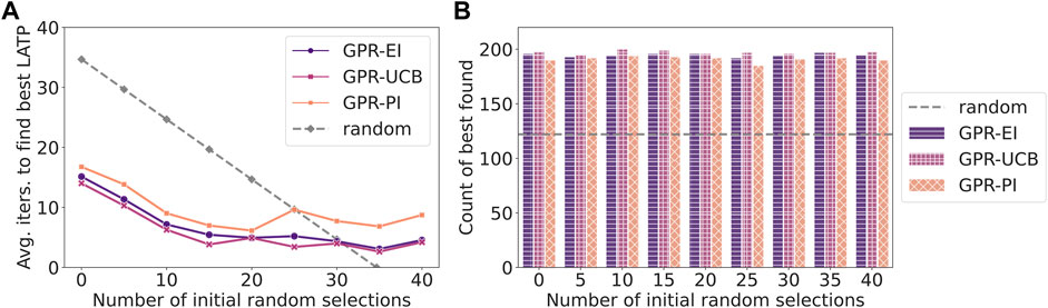
FIGURE 3. Comparison of GPR based Bayesian optimization with different acquisition functions, EI (dark purple), UCB (light purple), PI (orange) and random selection (grey dashed): (A) number of counts to find the global maximum in the repeated 200 virtual experiments, where random selection (grey dashed line) can find 126 times (63%); (B) number of additional tries of different strategies needed after n initial random selections (x-axis) to find the global maximum of ionic conductivity (1.09 × 10⁻³ S cm⁻¹) in the training data set (grid search). On average random selection takes about 34.7 tries to arrive at the maximum. It is noticeable that only those cases where the global minimum is found are counted to calculate the average.

3 Results and Discussions

3.1 Data Set

The initial 80 training data points are listed in Supplementary Table S1.

3.2 Model Selection

As there is no clear indication of which optimization strategy to use (according to the “no-free-lunch theorem” (Wolpert and Macready, 1997), there is no universal optimizer for all problems), we compare the optimization efficiencies of BOs with random search, EI, UCB and PI strategies with the 80 initial points from the grid search study. The strategy of achieving the maximum ionic conductivity (1.09 × 10⁻³ S cm⁻¹) with the least number of average iterations is considered to be optimal. During the experiment of comparing these strategies, random noise is added to the observations and the sample is allowed to be picked more than once (namely, with replacement). In detail, we randomly select a given number of samples from the training data with replacement as initial data points, then train the model using a given acquisition function and count the total number of extra tries (after initial random picks) needed to find the best sample (that is, the one with the largest ionic conductivity) in the grid search study. The model is only allowed to make up to m attempts (m = 80 − number of initial data points) to find the maximum value. This process is called “virtual experiment” and is repeated 200 times with different sets of randomly selected samples. In the overall count, the initial random picks are excluded. Detailed results of comparing different strategies of acquisition functions are shown in Figure 3.

Figure 3A illustrates how many times different strategies can find the global maximum (1.09 × 10⁻³ S cm⁻¹) within the 80 tries in 200 virtual experiments. The grey dashed line represents how many counts the random selection can find the global maximum. Among the 200 virtual experiments, the random selection can find 126 times (63%) and it acts as the base line for evaluating the performance of other models. From the figure it can be seen that GPR model with an EI (dark purple) or UCB (light purple) acquisition function can find the maximum in most virtual experiments $(\ge 95\%)$, where UCB performs slightly better than EI in some cases. In contrast, PI (orange) performs slightly worse than the other two, but still much better than the random selection. We speculate that PI sometimes gets stuck in the local optimum, making it difficult for the model to reach the global maximum. As a result, it fails to find the global maximum in some cases.

Figure 3B illustrates the average number of extra tries (after a given number of initial data points) required for the models with different acquisition functions to find the global maximum. The random selection takes on average 34.7 tries to find the global maximum, which is marked as grey dashed line in the figure. It can be seen that all the three models perform much better than the random selection. Performance of EI and UCB is similar, with UCB being slightly better and it takes the fewest extra tries to achieve the best result. More specifically, the number of extra tries needed to find the global maximum for EI and UCB decreases quickly with more initial data points, which is reasonable as the models’ ability to fit and predict is gradually enhanced. After more than 15 initial data points, the gain of introducing more initial data points gradually decreases and the required extra tries finally stabilizes at about 5. This phenomenon is very beneficial for experiments because the model can achieve good performance even with only a small number of initial data points, significantly reducing the number of attempts required. In contrast, the performance of PI is worse than the other two strategies as it requires more steps to obtain the global optimum. Therefore, we choose the model with UCB acquisition function and use it to predict the optimal experimental conditions, as it is more robust and takes fewer steps to reach the global optimum.

3.3 Result of Newly Synthesized Lithium Aluminum Titanium Phosphate Samples

As the search space becomes larger, it is difficult to manually determine the experimental conditions to obtain samples with better performance. Hence, a machine learning model is employed to help to explore the unknown experimental space quickly in order to reduce the number of required trials. The experimental conditions predicted by the model and their measured properties of the resulting new samples, namely, relative density after sintering and ionic conductivity, are listed in Table 2. All samples have a green density of approximately 62% so this property is not listed. Starting with 80 data points, we have performed 4 iterations (each predicting 5–6 samples) to optimize the experimental conditions to obtain LATP with higher ionic conductivity. At the end of each iteration, the newly synthesized samples are fed back to the model, which is then retrained. After the update, new experimental conditions are predicted for the next iteration. This process forms a loop, which is repeated until the target number of iterations has been achieved. In total 22 new samples are synthesized.

TABLE 2

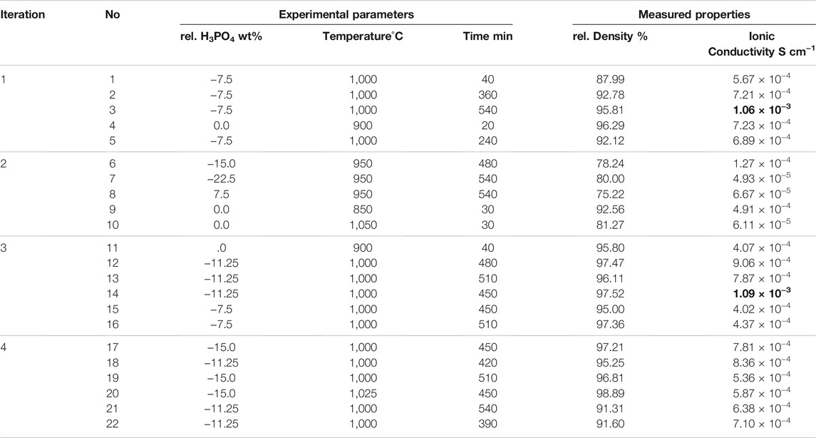
TABLE 2. Recommended samples using BO and measured properties.

It can be seen from Table 2 that the model quickly discovers a new sample (sample No. 3) with second highest ionic conductivity (1.06 × 10⁻³ S cm⁻¹) in the first iteration. The ionic conductivity of this sample is very close to the highest one of all samples (1.09 × 10⁻³ S cm⁻¹), which shows a very good performance of our model. The comparison of experimental conditions shows that even though the sintering time of the new sample (540 min) is 60 min longer than that of the known maximum sample (480 min, with a deficiency of −7.25% H₃PO₄ at 900°C), it can still maintain good performance. This indicates that LATP samples synthesized under this condition are stable against long holding time. On the other hand, comparing the densities of samples No. 2 (360 min) and No. 5 (240 min) it can be concluded that shorter holding time is not enough for the samples to get fully sintered as the densities of these samples are less than those with longer holding time. Therefore, the ionic conductivities of these samples are significantly lower than those of the fully sintered ones.

As the Bayesian optimization process is a trade-off process between exploration and exploitation, it is important to explore unknown areas efficiently, which can help to find the global optimum in a scientific way. This can be well reflected in our experiments. It can be seen that in the first iteration, the model explores experimental conditions with holding time at 360 min (sample No. 2) and 240 min (sample No. 5), as the original experimental conditions of grid search have a large gap (uncertainty) of holding time between 60 and 480 min. Similarly, this can also explain why the model in the second iteration explores the temperature intervals that have never been explored before, as these areas are subject to relatively large degrees of uncertainties. Though samples obtained in the second iteration show poor ionic conductivity (on average 1.59 × 10⁻⁴ S cm⁻¹), it does not render this iteration a failure. This attempt is reasonable and can help the model to quickly explore this unknown region and excludes the possibility of an optimal value appearing in that region, which effectively reduces the number of tries it needs compared to the exhaustive method. Notably, starting from the third iteration, we expand the range of experimental conditions that can be chosen, more centrally, we expand the extent to which the amount of precursor H₃PO₄ can be adjusted, as its preparation can take a long time. It can be clearly seen that the model also undergoes a competitive process between exploration and exploitation in the third and fourth iterations. It first makes predictions (samples No. 12–14) with experimental conditions with a deficiency of −11.25% H₃PO₄, which has never been explored before (exploration). At this point, the model finds a new sample (sample No. 14) with a value of ionic conductivity which is as large as the previous maximum (1.09 × 10⁻³ S cm⁻¹). Then the model begins to make the most of this information and makes several attempts (samples No. 18, 21, 22) around this point (exploitation). It can be seen that properties (ionic conductivity) of later samples are inferior to that of sample No. 14, indicating that the model has a good predictive performance. As a result, it can find the optimal value efficiently and quickly, reducing the number of required experiments.

The values of ionic conductivity (black line) during the four iterations and the values of the maximum (grey line) are plotted in Figure 4. It can be noted that the overall result shows a step-wise upward trend, illustrating the improvement of new samples during iterations. During the iteration, the model goes through a process of exploration and exploitation, which can be reflected in the fluctuating experimental results of ionic conductivity. The model first selects a sample which yields moderate performance (5.67 × 10⁻⁴ S cm⁻¹). Afterwards, the performance of samples increases with iterations and it quickly finds the second highest maximum (sample No. 3). Starting from the sample No. 11, the search space is extended (marked as the vertical grey dashed line in the middle) and the model quickly finds another global maximum (sample No. 14, marked as red star). Another schematic diagram (similar to Figure 2) is shown in the supporting material (Supplementary Figure S1) to illustrate the above working principle and to better visualize the evolution of changes in the predictions of the model during different iterations. Overall, results of predictions prove that our model has a good ability to help us to find another sample with maximum ionic conductivity under different experimental condition where it has never been explored before. By using the Bayesian optimization model, it can help the experimentalist to quickly narrow the search space and hence can reduce the number of required experiments effectively.

FIGURE 4

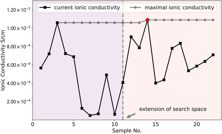
FIGURE 4. The values of ionic conductivity for each sample (black line) during the four iterations and the values of the maximum (grey line). The results of experiments show a fluctuating trend, reflecting the exploration vs. exploitation in the optimization process. The overall result exhibits a step-wise upward trend and it can be seen that the model has found the largest values of ionic conductivity (marked as red star) within several iterations.

To further explore why these samples (e.g., sample No. 14) have better performances than others, characterization measurement are performed to investigate the mechanisms governing the high ionic conductivity. Details are given in the next section.

3.4 Characterization of Lithium Aluminum Titanium Phosphate Samples

A standard stoichiometric LATP sample reaches the highest ionic conductivity at a sintering temperature of 900°C and a holding time of 30 min. With the aid of machine learning algorithms, the best properties are achieved for the sample No. 14, which is sintered from a LATP batch synthesized with a deficit of −11.25 wt% in phosphoric acid and sintered at 1,000°C for 450 min. For a better understanding why this sample has also reached ionic conductivity performance in the order of 1 × 10⁻³ S cm⁻¹, even though synthesis and sintering conditions deviated from the standard procedure, the microstructure is analyzed. Figure 5 shows a comparison of the X-ray diffraction patterns of the standard stoichiometric LATP (0.0 wt%) sample and another LATP (−11.25 wt%) sample. While the stoichiometric sample is still phase pure in the expected NZP-structure after sintering, clear foreign peaks can be seen in the LATP (−11.25 wt%) sample. Among the foreign phases that have formed in addition to the NZP-structure, TiO₂ could be identified as a second phase.

FIGURE 5

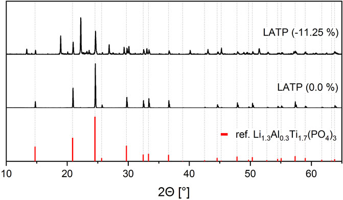
FIGURE 5. X-ray diffraction patterns for the LATP (−11.25 wt%) sample sintered at 1,000°C for 450 min and one LATP (0.0 wt%) sample sintered at 900°C for 30 min. A standard X-ray diffraction pattern of Li_1.3Al_0.3Ti_1.7(PO₄)₃ from the database is shown in red color for reference.

In addition, the different microstructure developments are shown in Figure 6. Figure 6A shows the LATP (0.0 wt%) sample sintered at 900°C with a holding time of 30 min. There, the ionic conductivity in the order of 1 × 10⁻³ S cm⁻¹ is achieved by a homogeneous and dense microstructure with small and uniform grains as well as very small and finely distributed pores. Despite the significantly different sintering parameters, Figure 6B shows a similar homogeneous microstructure with only slightly larger grains and pores for the LATP (−11.25 wt%) sample. The homogeneous grain size and dense structure is not typical for LATP sintered at this high temperature as the comparison in Figure 6C with LATP (0.0 wt%) sintered with these parameters shows. There, abnormal grain growth and the related microcracks in these large grains, due to a high thermal expansion anisotropy between a and c lattice parameters, shatter the microstructure and cause a drastic decrease in ionic conductivity (Jackman and Cutler, 2012; Hupfer et al., 2016; Waetzig et al., 2016). Grain growth seems to be suppressed for the LATP (−11.25 wt%) sample by second-phase particles, which are visible as homogeneously distributed bright dots throughout the structure at the triple points of the grain boundaries. The evaluation of the corresponding XRD-pattern leads to the assumption that the second phase is TiO₂ and this is reinforced by the results of the EDX (Energy dispersive X-Ray) analysis of one of these particles shown in Figure 7. The line-scan shows a clear increase in the titanium intensity in the EDX measurement at the position of the bright particle. The interaction between second-phase particles and migrating grain boundaries is known as Zener-type mechanism in ceramic materials and can reduce grain growth. This is likely to be the reason for the moderate grain growth of the LATP (−11.25 wt%) sample at these high sintering temperatures (Rahaman, 2007). It allows for a densification of the microstructure that in turn results in a ionic conductivity in the order of 1 × 10⁻³ S cm⁻¹. The above analysis serves to explain the possible mechanism why samples like No. 14 have better performances than others, which agrees well with the conclusions from our previous study (Schiffmann et al., 2021) where a deficiency of phosphoric acid in the synthesis can lead to the formation of LiTiOPO₄ and TiO₂. It seems that the second phases are the reason for the prevention of abnormal grain growth for sintering temperatures up to 1,000°C. Because the small grains are less susceptible to microcracking, a dense structure with high ionic conductivity is achievable even sintered at these high sintering temperatures. Experimental parameters for other samples, such as the sample No. 3 (1.06 × 10⁻³ S cm⁻¹) synthesized with parameters (−7.5 wt%, 1,000°C, 540 min), are comparable to one of the samples (−7.5 wt%, 1,000°C, 480 min with ionic conductivity of 1.09 × 10⁻³ S cm⁻¹) in the paper mentioned above and one can therefore assume that a comparable microstructure is the reason for the high ionic conductivity of this sample as well.

FIGURE 6

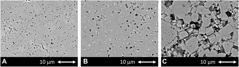
FIGURE 6. Microstructure of (A) LATP (0.0 wt%) sample sintered at 900°C for 30 min; (B) LATP (−11.25 wt%) sample sintered at 1,000°C for 450 min and (C) LATP (0.0 wt%) sample sintered at 1,000°C for 450 min.

FIGURE 7

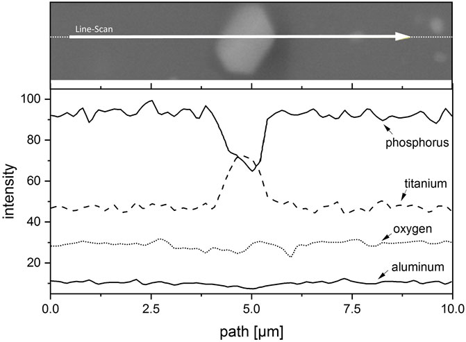
FIGURE 7. EDX-line-scan of a bright second phase particle in the structure of the sintered LATP (−11.25 wt%) sample. A significant increase can be clearly seen in titanium intensity at the position of the bright region, which indicates that the second phase is highly possible to be TiO₂.

4 Conclusion

Our work shows that a data-driven materials design strategy based on Bayesian optimization using Gaussian process regression can be employed in effectively designing experimental conditions for synthesizing LATP, which is one of the potential solid electrolyte candidates for batteries. The whole design strategy is divided into several sections: first, to find the most suitable model for our study, virtual experiments are performed to compare models built with several combinations of design strategies using the training data assembled from previous laboratory studies. In our study, we find that the model with UCB (upper confidence boundary) strategy can achieve the best performance. Second, the best model is then selected to design new experimental parameters in order to synthesize new sample with the largest possible value of ionic conductivity. Third, the corresponding properties of the newly sintered samples are measured and these results are fed back to update the model for the next iteration of the design process. Our results show that within several iterations, newly synthesized samples guided by the model can achieve a good performance with maximum value of 1.09 × 10⁻³ S cm⁻¹, which is in the same order of magnitude of the maximum Li-ion conductivity that LATP can achieve. In addition, the range of search space can be dynamically adjusted during the experiment, making this method flexible according to researchers’ needs. Besides, it can help the researcher to quickly explore the boundary of the range of experimental parameters which may yield samples with good performance, hence it can be assisted in designing experiments in an effective and reasonable way to reduce the number of required experiments. It is worth noting here that the main focus of this work is on single-objective optimization, that is, only the ionic conductivity is paid attention to. Admittedly, this is a simplification of the optimization problem, since other properties (e.g., sintered density) can also affect our interested property. As a result, taking them into consideration and regarding it as a multi-objective optimization problem (previous studies concerning similar question can be found in (Harada et al., 2020; Yang et al., 2020)) may further improve the performance of the model and may hence result in better samples. This question deserves to be explored in details and is left for the future research.

In order to further understand the reasons governing the high ionic conductivity of these samples, the resulting crystal structures and phase compositions are studied with X-ray diffraction and energy dispersive X-Ray analysis, while the microstructures of sintered pellets are investigated by scanning electron microscopy. The formation of secondary phases such as TiO₂, is demonstrated to be substantially influenced by the initial concentration of the precursors, which can influence ionic conductivity, densification behavior, and microstructure evolution.

In summary, our studies demonstrate the advantages of adopting machine learning for an accelerated design of experimental parameters by the synthesis of materials with targeted properties, which can help experimentalists to explore the search space effectively and narrow the parameter range quickly. This is a general method that can be mapped to other research systems and the whole workflow will be kept sustainable within the Kadi4Mat framework, which can reduce the number of required experiments and accelerate the process of developing materials.

Data Availability Statement

The original contributions presented in the study are included in the article/Supplementary Material, further inquiries can be directed to the corresponding author.

Author Contributions

All authors listed have made a substantial, direct, and intellectual contribution to the work and approved it for publication.

Funding

This work is supported by the German Federal Ministry of Education and Research (BMBF) within the “FESTBATT” consortium (Grant No. 03XP0174E). Contribution to the integration of the methods into the Kadi4Mat research data infrastructure is provided by the Helmholtz Association of German Research Centres through the program “MTET” (Grant No. 38.02.01).

Conflict of Interest

The authors declare that the research was conducted in the absence of any commercial or financial relationships that could be construed as a potential conflict of interest.

Publisher’s Note

All claims expressed in this article are solely those of the authors and do not necessarily represent those of their affiliated organizations, or those of the publisher, the editors and the reviewers. Any product that may be evaluated in this article, or claim that may be made by its manufacturer, is not guaranteed or endorsed by the publisher.

Supplementary Material

The Supplementary Material for this article can be found online at: https://www.frontiersin.org/articles/10.3389/fmats.2022.821817/full#supplementary-material

References

Ahmad, Z., Xie, T., Maheshwari, C., Grossman, J. C., and Viswanathan, V. (2018). Machine Learning Enabled Computational Screening of Inorganic Solid Electrolytes for Suppression of Dendrite Formation in Lithium Metal Anodes. ACS Cent. Sci. 4, 996–1006. doi:10.1021/acscentsci.8b00229

PubMed Abstract | CrossRef Full Text | Google Scholar

Alberi, K., Nardelli, M. B., Zakutayev, A., Mitas, L., Curtarolo, S., Jain, A., et al. (2018). The 2019 Materials by Design Roadmap. J. Phys. D Appl. Phys. 52, 013001. doi:10.1088/1361-6463/aad926

CrossRef Full Text | Google Scholar

Aono, H., Sugimoto, E., Sadaoka, Y., Imanaka, N., and Adachi, G.-y. (1990). Ionic Conductivity and Sinterability of Lithium Titanium Phosphate System. Solid State Ionics 40-41, 38–42. doi:10.1016/0167-2738(90)90282-v

CrossRef Full Text | Google Scholar

Aravindan, V., Gnanaraj, J., Madhavi, S., and Liu, H.-K. (2011). Lithium-ion Conducting Electrolyte Salts for Lithium Batteries. Chem. Eur. J. 17, 14326–14346. doi:10.1002/chem.201101486

PubMed Abstract | CrossRef Full Text | Google Scholar

Arbi, K., Mandal, S., Rojo, J. M., and Sanz, J. (2002). Dependence of Ionic Conductivity on Composition of Fast Ionic Conductors Li1+xTi2-xAlx(PO4)3, 0 ≤ X ≤ 0.7. A Parallel NMR and Electric Impedance Study. Chem. Mater. 14, 1091–1097. doi:10.1021/cm010528i

CrossRef Full Text | Google Scholar

Auer, P., Cesa-Bianchi, N., and Fischer, P. (2002). Finite-time Analysis of the Multiarmed Bandit Problem. Machine Learn. 47, 235–256. doi:10.1023/a:1013689704352

CrossRef Full Text | Google Scholar

Brandt, N., Griem, L., Herrmann, C., Schoof, E., Tosato, G., Zhao, Y., et al. (2021). Kadi4mat: A Research Data Infrastructure for Materials Science. Data Sci. J. 20. doi:10.5334/dsj-2021-008

CrossRef Full Text | Google Scholar

Brochu, E., Cora, V. M., and De Freitas, N. (2010). A Tutorial on Bayesian Optimization of Expensive Cost Functions, with Application to Active User Modeling and Hierarchical Reinforcement Learning. arXiv. arXiv preprint arXiv:1012.2599.

Google Scholar

Bucharsky, E. C., Schell, K. G., Hintennach, A., and Hoffmann, M. J. (2015). Preparation and Characterization of Sol-Gel Derived High Lithium Ion Conductive NZP-type Ceramics Li1+x AlxTi2−x(PO4)3. Solid State Ionics 274, 77–82. doi:10.1016/j.ssi.2015.03.009

CrossRef Full Text | Google Scholar

Cohn, D. A., Ghahramani, Z., and Jordan, M. I. (1996). Active Learning with Statistical Models. JAIR 4, 129–145. doi:10.1613/jair.295

CrossRef Full Text | Google Scholar

Coley, C. W., Eyke, N. S., and Jensen, K. F. (2020). Autonomous Discovery in the Chemical Sciences Part Ii: Outlook. Angew. Chem. Int. Ed. 59, 23414–23436. doi:10.1002/anie.201909989

CrossRef Full Text | Google Scholar

Cressie, N. (1990). The Origins of Kriging. Math. Geol. 22, 239–252. doi:10.1007/bf00889887

CrossRef Full Text | Google Scholar

Frazier, P. I. (2018). A Tutorial on Bayesian Optimization. arXiv. arXiv preprint arXiv:1807.02811.

Google Scholar

Fujimura, K., Seko, A., Koyama, Y., Kuwabara, A., Kishida, I., Shitara, K., et al. (2013). Accelerated Materials Design of Lithium Superionic Conductors Based on First-Principles Calculations and Machine Learning Algorithms. Adv. Energ. Mater. 3, 980–985. doi:10.1002/aenm.201300060

CrossRef Full Text | Google Scholar

Goodenough, J. B., and Kim, Y. (2010). Challenges for Rechargeable Li Batteries. Chem. Mater. 22, 587–603. doi:10.1021/cm901452z

CrossRef Full Text | Google Scholar

Häse, F., Roch, L. M., and Aspuru-Guzik, A. (2019). Next-generation Experimentation with Self-Driving Laboratories. Trends Chem. 1, 282–291. doi:10.1016/j.trechm.2019.02.007

CrossRef Full Text | Google Scholar

Harada, M., Takeda, H., Suzuki, S., Nakano, K., Tanibata, N., Nakayama, M., et al. (2020). Bayesian-optimization-guided Experimental Search of Nasicon-type Solid Electrolytes for All-Solid-State Li-Ion Batteries. J. Mater. Chem. A. 8, 15103–15109. doi:10.1039/d0ta04441e

CrossRef Full Text | Google Scholar

Homma, K., Liu, Y., Sumita, M., Tamura, R., Fushimi, N., Iwata, J., et al. (2020). Optimization of a Heterogeneous Ternary Li3PO4-Li3BO3-Li2SO4 Mixture for Li-Ion Conductivity by Machine Learning. J. Phys. Chem. C 124, 12865–12870. doi:10.1021/acs.jpcc.9b11654

CrossRef Full Text | Google Scholar

Hupfer, T., Bucharsky, E. C., Schell, K. G., Senyshyn, A., Monchak, M., Hoffmann, M. J., et al. (2016). Evolution of Microstructure and its Relation to Ionic Conductivity in Li1+xAlxTi2−x(PO4)3. Solid State Ionics 288, 235–239. doi:10.1016/j.ssi.2016.01.036

CrossRef Full Text | Google Scholar

Hupfer, T., Bucharsky, E. C., Schell, K. G., and Hoffmann, M. J. (2017). Influence of the Secondary Phase LiTiOPO 4 on the Properties of Li 1+x Al X Ti 2−x (PO 4 ) 3 (X = 0; 0.3). Solid State Ionics 302, 49–53. doi:10.1016/j.ssi.2016.10.008

CrossRef Full Text | Google Scholar

Jackman, S. D., and Cutler, R. A. (2012). Effect of Microcracking on Ionic Conductivity in Latp. J. Power Sourc. 218, 65–72. doi:10.1016/j.jpowsour.2012.06.081

CrossRef Full Text | Google Scholar

Jalem, R., Kanamori, K., Takeuchi, I., Nakayama, M., Yamasaki, H., and Saito, T. (2018). Bayesian-driven First-Principles Calculations for Accelerating Exploration of Fast Ion Conductors for Rechargeable Battery Application. Sci. Rep. 8, 5845–5910. doi:10.1038/s41598-018-23852-y

PubMed Abstract | CrossRef Full Text | Google Scholar

Jones, D. R., Schonlau, M., and Welch, W. J. (1998). Efficient Global Optimization of Expensive Black-Box Functions. J. Glob. Optimizat. 13, 455–492. doi:10.1023/a:1008306431147

CrossRef Full Text | Google Scholar

Ki Williams, C. (2006). Gaussian Processes Formachine Learning. Taylor & Francis Group.

Google Scholar

Kushner, H. J. (1964). A New Method of Locating the Maximum point of an Arbitrary Multipeak Curve in the Presence of Noise. J. Basic Eng. 86 (1), 97–106. doi:10.1115/1.3653121

CrossRef Full Text | Google Scholar

Ma, Q., Xu, Q., Tsai, C.-L., Tietz, F., and Guillon, O. (2016). A Novel Sol-Gel Method for Large-Scale Production of Nanopowders: Preparation of Li1.5Al0.5Ti1.5(PO4)3as an Example. J. Am. Ceram. Soc. 99, 410–414. doi:10.1111/jace.13997

CrossRef Full Text | Google Scholar

MacLeod, B. P., Parlane, F. G. L., Morrissey, T. D., Häse, F., Roch, L. M., Dettelbach, K. E., et al. (2020). Self-driving Laboratory for Accelerated Discovery of Thin-Film Materials. Sci. Adv. 6, eaaz8867. doi:10.1126/sciadv.aaz8867

PubMed Abstract | CrossRef Full Text | Google Scholar

Manthiram, A., Yu, X., and Wang, S. (2017). Lithium Battery Chemistries Enabled by Solid-State Electrolytes. Nat. Rev. Mater. 2, 1–16. doi:10.1038/natrevmats.2016.103

CrossRef Full Text | Google Scholar

Močkus, J. (1975). “On Bayesian Methods for Seeking the Extremum,” in Optimization Techniques IFIP Technical Conference (Springer), 400–404.

Google Scholar

Narváez-Semanate, J. L., and Rodrigues, A. C. M. (2010). Microstructure and Ionic Conductivity of Li1+Al Ti2−(PO4)3 NASICON Glass-Ceramics. Solid State Ionics 181, 1197–1204. doi:10.1016/j.ssi.2010.05.010

CrossRef Full Text | Google Scholar

Pérez-Estébanez, M., Isasi-Marín, J., Többens, D. M., Rivera-Calzada, A., and León, C. (2014). A Systematic Study of Nasicon-type Li1+xMxTi2−x(PO4)3 (M: Cr, Al, Fe) by Neutron Diffraction and Impedance Spectroscopy. Solid State Ionics 266, 1–8. doi:10.1016/j.ssi.2014.07.018

CrossRef Full Text | Google Scholar

Rahaman, M. N. (2007). Sintering of Ceramics. CRC Press.

Google Scholar

Rasmussen, C. E. (2003). “Gaussian Processes in Machine Learning,” in Summer School on Machine Learning (Springer), 63–71.

Google Scholar

Rohr, B., Stein, H. S., Guevarra, D., Wang, Y., Haber, J. A., Aykol, M., et al. (2020). Benchmarking the Acceleration of Materials Discovery by Sequential Learning. Chem. Sci. 11, 2696–2706. doi:10.1039/c9sc05999g

PubMed Abstract | CrossRef Full Text | Google Scholar

Rossbach, A., Tietz, F., and Grieshammer, S. (2018). Structural and Transport Properties of Lithium-Conducting Nasicon Materials. J. Power Sourc. 391, 1–9. doi:10.1016/j.jpowsour.2018.04.059

CrossRef Full Text | Google Scholar

Schiffmann, N., Bucharsky, E. C., Schell, K. G., Fritsch, C. A., Knapp, M., and Hoffmann, M. J. (2021). Upscaling of Latp Synthesis: Stoichiometric Screening of Phase Purity and Microstructure to Ionic Conductivity Maps. Ionics 27, 2017–2025. doi:10.1007/s11581-021-03961-x

CrossRef Full Text | Google Scholar

Sendek, A. D., Yang, Q., Cubuk, E. D., Duerloo, K.-A. N., Cui, Y., and Reed, E. J. (2017). Holistic Computational Structure Screening of More Than 12 000 Candidates for Solid Lithium-Ion Conductor Materials. Energy Environ. Sci. 10, 306–320. doi:10.1039/c6ee02697d

CrossRef Full Text | Google Scholar

Shahriari, B., Swersky, K., Wang, Z., Adams, R. P., and De Freitas, N. (2015). Taking the Human Out of the Loop: A Review of Bayesian Optimization. Proc. IEEE 104, 148–175. doi:10.1109/JPROC.2015.2494218

CrossRef Full Text | Google Scholar

Snoek, J., Larochelle, H., and Adams, R. P. (2012). Practical Bayesian Optimization of Machine Learning Algorithms. arXiv. arXiv preprint arXiv:1206.2944.

Google Scholar

Srinivas, N., Krause, A., Kakade, S. M., and Seeger, M. (2009). Gaussian Process Optimization in the Bandit Setting: No Regret and Experimental Design. arXiv. arXiv preprint arXiv:0912.3995.

Google Scholar

Stein, H. S., and Gregoire, J. M. (2019). Progress and Prospects for Accelerating Materials Science with Automated and Autonomous Workflows. Chem. Sci. 10, 9640–9649. doi:10.1039/c9sc03766g

PubMed Abstract | CrossRef Full Text | Google Scholar

Tran, K., and Ulissi, Z. W. (2018). Active Learning across Intermetallics to Guide Discovery of Electrocatalysts for CO2 Reduction and H2 Evolution. Nat. Catal. 1, 696–703. doi:10.1038/s41929-018-0142-1

CrossRef Full Text | Google Scholar

Vasudevan, R. K., Choudhary, K., Mehta, A., Smith, R., Kusne, G., Tavazza, F., et al. (2019). Materials Science in the Artificial Intelligence Age: High-Throughput Library Generation, Machine Learning, and a Pathway from Correlations to the Underpinning Physics. MRS Commun. 9, 821–838. doi:10.1557/mrc.2019.95

CrossRef Full Text | Google Scholar

Waetzig, K., Rost, A., Langklotz, U., Matthey, B., and Schilm, J. (2016). An Explanation of the Microcrack Formation in Li 1.3 Al 0.3 Ti 1.7 (PO 4 ) 3 Ceramics. J. Eur. Ceram. Soc. 36, 1995–2001. doi:10.1016/j.jeurceramsoc.2016.02.042

CrossRef Full Text | Google Scholar

Wang, Y., Richards, W. D., Ong, S. P., Miara, L. J., Kim, J. C., Mo, Y., et al. (2015). Design Principles for Solid-State Lithium Superionic Conductors. Nat. Mater 14, 1026–1031. doi:10.1038/nmat4369

PubMed Abstract | CrossRef Full Text | Google Scholar

Williams, C. K., and Rasmussen, C. E. (2006). Gaussian Processes for Machine Learning, Vol. 2. Cambridge, MA: MIT press.

Google Scholar

Wolpert, D. H., and Macready, W. G. (1997). No Free Lunch Theorems for Optimization. IEEE Trans. Evol. Computat. 1, 67–82. doi:10.1109/4235.585893

CrossRef Full Text | Google Scholar

Xue, D., Balachandran, P. V., Hogden, J., Theiler, J., Xue, D., and Lookman, T. (2016). Accelerated Search for Materials with Targeted Properties by Adaptive Design. Nat. Commun. 7, 11241–11249. doi:10.1038/ncomms11241

PubMed Abstract | CrossRef Full Text | Google Scholar

Yang, Z., Suzuki, S., Tanibata, N., Takeda, H., Nakayama, M., Karasuyama, M., et al. (2020). Efficient Experimental Search for Discovering a Fast Li-Ion Conductor from a Perovskite-type LixLa(1-x)/3NbO3 (LLNO) Solid-State Electrolyte Using Bayesian Optimization. J. Phys. Chem. C 125, 152–160. doi:10.1021/acs.jpcc.0c08887

CrossRef Full Text | Google Scholar

Yuan, R., Tian, Y., Xue, D., Xue, D., Zhou, Y., Ding, X., et al. (2019). Accelerated Search for BaTiO 3 ‐Based Ceramics with Large Energy Storage at Low Fields Using Machine Learning and Experimental Design. Adv. Sci. 6, 1901395. doi:10.1002/advs.201901395

PubMed Abstract | CrossRef Full Text | Google Scholar

Zhang, Y., He, X., Chen, Z., Bai, Q., Nolan, A. M., Roberts, C. A., et al. (2019). Unsupervised Discovery of Solid-State Lithium Ion Conductors. Nat. Commun. 10, 5260–5267. doi:10.1038/s41467-019-13214-1

PubMed Abstract | CrossRef Full Text | Google Scholar