 Youdong Zhang
 Guijian Xiao
95% of researchers rate our articles as excellent or good
Learn more about the work of our research integrity team to safeguard the quality of each article we publish.
Find out more
ORIGINAL RESEARCH article
Front. Mater. , 13 May 2022
Sec. Environmental Degradation of Materials
Volume 9 - 2022 | https://doi.org/10.3389/fmats.2022.765401
This article is part of the Research Topic Machining Technology and Environmental Degradation Mechanism of Surface Microstructure of Special Materials View all 10 articles
Abrasive belt grinding has unique advantages in avoiding machining defects and improving surface integrity while grinding hard materials such as superalloys. However, the random distribution of abrasive particles on the abrasive belt surface is uncontrollable, and chatter and machining errors accompany the machining process, leading to unclear mapping relationship between process parameters and surface roughness, which brings great challenges to the prediction of surface roughness of superalloy. Traditional empirical equations are highly dependent on empirical knowledge and the development of scientific theories and can only solve problems with relatively simple and clear mechanisms, but cannot effectively solve complex and mutually coupled problems. The method based on data-driven patterns has a better idea for mining the implicit mapping relationship and eliminating the uncertainty of complex problems. This study presents a data-driven roughness prediction method for GH4169 superalloy. First, a superalloy grinding platform is built. According to the grinding empirical equation, the mapping relationship between process parameters and surface roughness is analyzed, and a prediction model is established based on the error back propagation (BP) algorithm. Second, genetic algorithm (GA) and particle swarm optimization (PSO) algorithm are used to optimize the weights and thresholds of the neural network, and the global optimal solution is obtained. Finally, the prediction performance of different algorithms is compared. The results show that the non-uniform absolute errors of the BP algorithm, GA-BP algorithm, and PSO-BP algorithm are 0.12, 0.085, and 0.078, respectively. The results show that the roughness prediction algorithm based on PSO-BP is more suitable for GH4169 superalloy.
High-temperature alloys have been widely used in the aerospace field due to their high strength and good oxidation resistance. At present, the high-temperature alloy materials are mainly processed by die forging and precision milling, while this processing method inevitably has defects such as thermal stress concentration and large plastic deformation, which also leads to tool adhesion and chatter. In turn, it is easy for the large force to cause some surface defects such as burns, micro-cracks, and tensile stress on the surface of the workpiece, which makes it difficult to ensure the surface integrity of the parts (Zhu et al., 2020). Abrasive belt grinding can effectively improve the surface quality of superalloy materials with the advantages of low temperature and strong vibration absorption performance, so it has been widely applied in aeronautic and astronautic fields (Huang et al., 2016; Xiao et al., 2021; Xiao et al., 2022; Zhou et al., 2022).
Since the surface integrity of components has an important impact on their fatigue life, it can improve the surface integrity and performance of the workpiece (Li et al., 2022; Gao et al., 2021). The surface topography after grinding has an important influence on the service performance (Cui et al., 2021). Among them, the surface roughness has an important influence on the surface properties of the workpiece after processing (Zhang et al., 2020). Obtaining surface roughness is the main unfavorable factor affecting the fatigue life of the workpiece. By analyzing the surface roughness, topography characteristics, and residual stress distribution of the workpiece, the influence of surface integrity characteristics on fatigue life is studied. At the same time, a method to improve fatigue life by optimizing process parameters is proposed (Wang et al., 2020). Considering the stress concentration on the surface of the external load and the residual stress of shot peening, the position of the dangerous section after processing was calculated, and experimental verification is also conducted. In the above research, it is found that better surface quality can improve the service life of the workpiece. The prediction of the surface integrity characteristics can ensure that the workpiece can be replaced in time, minimize the loss of resources, and achieve sustainability development.
However, due to the uneven distribution of abrasives, there is inherently weak rigidity, as well as the high degree of nonlinearity and coupling in the grinding process parameters and surface roughness, resulting in unstable surface characteristics after grinding. At present, there are two kinds of main predictions for the roughness of the ground surface.
The traditional surface roughness prediction method is to use online monitoring and surface inspection after grinding to analyze the grinding mechanism and then build a physical model of the surface roughness after grinding. A force-based temperature modeling method is proposed to predict the surface integrity of nickel-based alloy broaching (Klocke et al., 2014). Theoretical and experimental research studies are carried out on the polishing mechanism of complex curved parts, and the roughness prediction model is obtained (Slatineanu et al., 2010; Huang et al., 2020; Huang et al., 2018). A preliminary analysis of the weak stiffness characteristics of the system is carried out, and the vibration mechanism of the system is revealed from the perspective of dynamic analysis. On the basis of the theoretical model, the stable conditions and factors affecting the processing stability are put forward by analyzing the influence of important factors. According to the adjustment of the grinding parameters, the optimization of the surface roughness is realized. Using numerical simulation and advanced measurement methods to study the surface characteristics and formation process of the method of micro-stiffener belt polishing (MSBP) titanium alloys has become a new method (Xiao and Huang, 2019). In addition, different surface characteristics can be obtained by adjusting the feed velocity and pressure. The surface contour line is obtained through the contour map, and the surface roughness distribution is obtained according to the contour line. The experimental results show that the surface characteristics, surface morphology, surface roughness, and residual stress all meet the given requirements. However, this method still has some limitations. The prediction accuracy, the generalization ability, and the transferability of the method are relatively low, so it is difficult to adapt to the complex grinding conditions.
With the development of artificial intelligence, many domestic and foreign researchers have applied the intelligent algorithms to the processing predictions. These intelligent algorithms have incomparable advantages in dealing with nonlinear, fuzzy, and unclear pattern features and high coupling problems. At the same time, these algorithms can also achieve accurate prediction of processing results. The input features of the algorithm are very important for predicting the results, and the selection of features can currently rely on sensor and machine data to build a multi-feature hybrid input model. Input features are selected by analyzing the correlation between input features and surface roughness, as well as hardware and time costs (Guo et al., 2021). A sequential deep learning framework long and short-term memory (LSTM) network was used to predict surface roughness. The convergence of the GA is relatively high, and the self-adaptive characteristics of the GA can be used to predict the surface roughness after processing (Cao et al., 2020). Experiments proved that this method could effectively improve grinding efficiency and obtain better surface roughness. By taking the grinding wheel velocity, workpiece velocity, cutting depth, and grinding wheel material as the research objects, production cost, production rate, and surface roughness are taken as the optimization goals. In the actual machining process, the influence of tool wear on the surface roughness is very important, and it has become the main trend to properly consider the real-time state of the tool in the algorithm (Xu et al., 2020). With the breakthrough of deep learning theory, the prediction method of grinding roughness based on the deep learning algorithm can effectively improve the prediction accuracy (Alavijeh and Amirabadi, 2019). In recent years, error back propagation (BP) has been used to predict tool life, and the radial basis function (RBF) network model are excellent in approximation ability, learning rate, and so on (Ding et al., 2010). At present, surface roughness prediction based on BP neural network algorithm is the key direction (Wu, 2007). Many experts at home and abroad have adopted the RBF network model to solve complex engineering problems. At the same time, other evolutionary algorithms are used to optimize the original model, and the model parameter values are dynamically optimized to improve the performance of the model (Gu et al., 2021; Zhang et al., 2012). The sensor is used to monitor the processing process in real time, process and analyze the detection signal, and propose the signal characteristics. The constructed roughness prediction model can further expand the application prospect (Pandiyan et al., 2018). Chang et al. used the experimental data as the training parameters of the SVM model by using bearings as materials for belt grinding experiments (Chang et al., 2019). This model could effectively shorten the grinding process optimization time and obtain the global optimal solution of the grinding surface integrity. However, the adjustment range of the radial basis center and other parameters was small during the correction process, and it was easy to fall into the local optimal solution, which restricted the generalization ability of RBF. The research shows that the improved particle swarm algorithm and the GA with excellent search performance are used to optimize the RBF parameters, search the optimal parameters in a wider range, and improve the prediction performance of the model (Golbabai and Mohebianfar, 2017).
The abrasive belt is a particular form of a coated belt, which is intensified by a tensioning mechanism and a driven wheel to make it move at a high velocity. It can achieve grinding by the workpiece’s shape, processing requirements, the shape of the workpiece, and processing requirements. Besides, belt grinding is widely known as precision machining because of its high material removal precision (the highest accuracy can reach 0.1 µm), flexible machining, and other characteristics. It has significant advantages for the precision machining of some typical difficult-to-machine materials.
Figure 1 is the material removal model of belt grinding. The abrasive belt attached to the driving wheel moves with the rotation of the wheel. Abrasive particles perform micro-cutting and removal of material on the surface of the workpiece material. The results show that the grinding parameters such as belt linear velocity, feed velocity, grinding pressure, and grinding depth have great influence on the surface integrity of the workpiece.
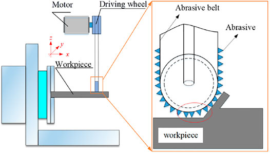
FIGURE 1. Belt grinding system.
The scholars in the previous research study have constructed the mathematical model of process parameters and surface roughness, as shown in Eq. 1:
where Ra is the surface roughness, vs is the linear belt velocity, vf is the feed velocity, Fn is the grinding pressure, ds is the grinding depth, P1 is the constant, and m, n, p, and q are relevant indexes. According to empirical Eq. 1, Ra is related to vs, vf, Fn, and ds, and the four parameters are highly nonlinear and highly coupled.
Due to the characteristics of abrasive grains and the influence of processing, there are significant problems in constructing the mathematical model between process parameters and Ra. The prediction accuracy has always restricted the development of roughness prediction. However, the traditional back propagation (BP) algorithm causes some iterations to fall into the optimal local solution due to the influence of the characteristics of the algorithm. The PSO algorithm and GA are introduced to optimize the BP algorithm’s initial weight and threshold to avoid the optimal local solution and obtain the optimal global solution. Simultaneously, the predicted results error after grinding is controlled within 5.00% to make the predicted value as accurate as possible. According to previous studies, linear belt velocity, feed velocity, grinding pressure, and grinding depth are the main factors that affect the surface roughness of the workpiece. The prediction model will give the surface roughness values obtained under the same grinding environment and grinding time for these four parameters. The grinding process parameters vs, vf, Fn, and ds are taken as the input of the neural network, and the surface roughness was taken as the output.
Figure 2 shows the topology of the neural network. According to the principle of the neural network algorithm, the number of neurons in the hidden layer p is determined by the following empirical function:
where p is the number of neurons in the hidden layer, n represents the number of input layers, and a represents a random value. For the convenience of calculation, the value is 10. According to the empirical Eq. 2, we choose 12 neurons in the hidden layer. x is the input vector, y is the output vector, w is the connection weight vector, b is the bias of the neural network, and f(x) is the activation function. f1(x) = tanhx and f2(x) = x are taken as activation functions of the hidden layer and the output layer, respectively.
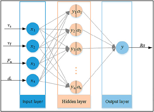
FIGURE 2. Propagation process diagram of the neural network.
For a given training set D = {(xk, yk): xk = [xk1, xk2,⋯, xkn ]T, y = [yk1, yk2, ⋯, ykm]T, k = 1, 2, ⋯, N}, and for a training sample (xj, yj)∈D. Neural network forward propagation method. Input layer: xj = [xj1, xj2, ⋯, xjn]T. Hidden layer: input vector x as the input vector. The neuron in the kth hidden layer has the connection weight w1k = [w1k1, w1k2, ⋯, w1kp] and the offset b2k. The output hk is given by Eq. 4:
Use the output value of all neurons hj = [hj1, hj2, ⋯, hjp]T as the output vector of the entire network. The first k of output layer neurons has the right to connect w2k = [w2k1, w2k2, ⋯, w2kp] and offset b2k, output
For a training case, the prediction accuracy of the training cases is evaluated as an index of Eq. 6:
Ej represents the loss function,
For the whole training example, the prediction accuracy is measured by the mean square error (MSE):
Before the neural network algorithm is trained, all the connection weights and thresholds are usually generated randomly by using the normal distribution. This makes the training effect of a simple BP neural network unstable. In order to improve the training effect of the algorithm, GA and PSO can be used to optimize the initial weight and threshold value of the neural network algorithm to the neural network, so that the iterative process is at a better starting point and many local optimal solutions can be avoided before the training iteration (Figure 3). The neural network iteration converges to a better local optimal solution or optimal global solution. Therefore, surface roughness can achieve higher accuracy and prediction accuracy based on the current data.
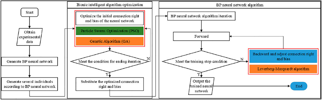
FIGURE 3. Flow chart of BP neural network optimization algorithm.
PSO algorithm is applied to construct a new vector because of BP algorithm connection weights and thresholds:
where µi represents the moving speed of each particle, and U represents the set of moving speeds of all particles. According to the principle of the algorithm, the computer randomly generates the initial position and speed according to the normal distribution. In particle motion, it is assumed that the ith particle’s proven optimal solution is pi, and all particles’ proven global optimal solution is G.
During the iteration of the algorithm, the velocity change of the ith particle is closely related to the particle’s current position. Using the optimization method of the PSO algorithm, the optimal global solution of particles is obtained as follows:
where w is the weight of the particle, c1 is the individual learning factor, c2 is the group learning factor, and a1 and a2 are random numbers. After the particle velocity vector is iteratively updated, the particle moves immediately. The new position of the particle is shown in Eq. 10:
After several iterations, all particles tend to move toward the optimal global solution. Simultaneously, the GA can be used for the optimization of complex systems and has better robustness. Compared with the traditional optimization method, it can directly take fitness as the search information, uses the search information of multiple points, and has implicit parallelism characteristics.
The GA optimizes the initial weights and thresholds. Using the characteristics of GA to optimize the initial parameters of BP algorithm can avoid the problem of local optimum caused by random parameters.
It comprises five parts: the input layers and the hidden layers, weight, threshold, and output layer. The difference between the predicted value and the expected value of the sample is selected as the error value, the obtained error value is formed into an error matrix, and the norm of the matrix is used as the objective function. The fitness function adopts the sorting of the appropriate allocation function. The selection operator simulates the “survival of the fittest,” selects highly adaptable individuals, increases relevant weights, and inherits these individuals to the next generation.
The basic steps of the GA algorithm are as follows:
1) In this study, the fitness function uses training data to train the BP neural network, and the prediction error of training data is regarded as the individual fitness value.
2) The selection operation uses roulette to select individuals with good fitness from the population to form a new population.
3) In crossover operation, two individuals are selected from the population and a new individual is obtained by crossing at a certain intersection.
4) Mutation operation selects an individual randomly from the population and obtains a new individual according to a certain probability of mutation.
On the contrary, particles with poor adaptability will be given a smaller weight and will not be inherited by the next generation during the training process. In this study, the roulette selection method is chosen. ΣFi represents the sum of the population’s fitness function, and fi represents the fitness value of the ith chromosome of the people. The ratio of fitness to offspring is fi/ΣFi.
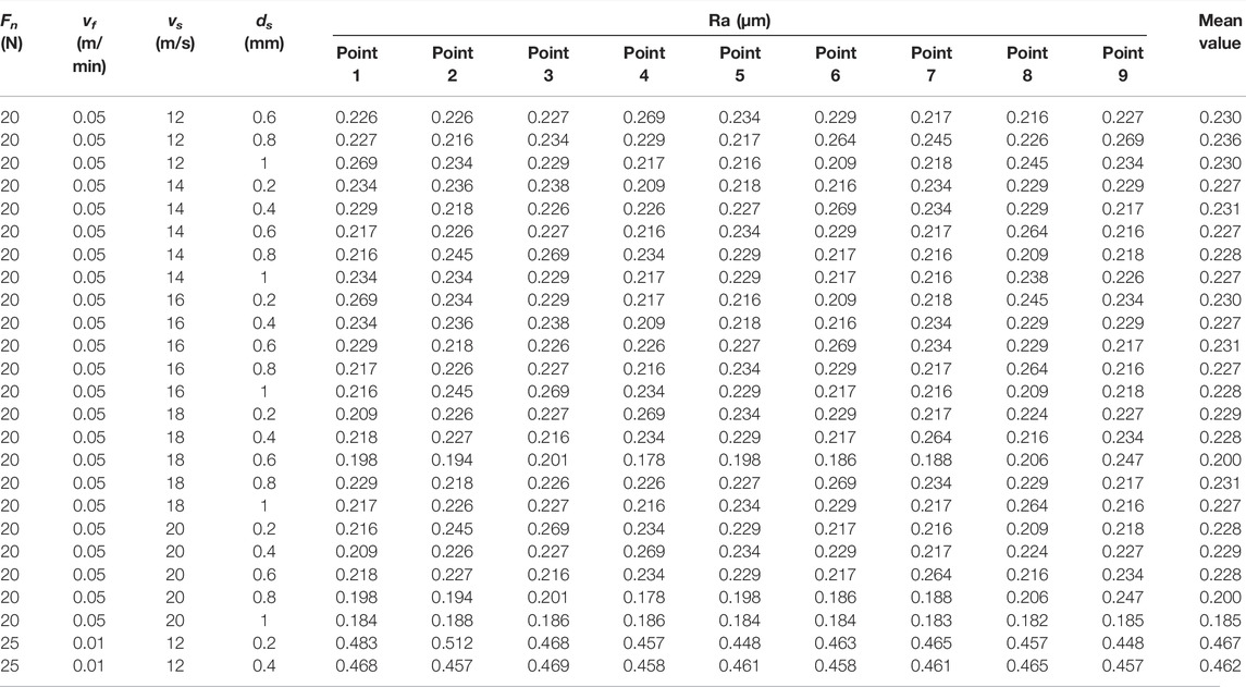
Figure 4 is the test equipment and surface roughness detection diagram. A seven-axis six-link abrasive belt grinder is used to grind the workpiece, and a roughness profiler is used to detect the workpiece. The grinding surface under different process parameters was detected by using a testing instrument, and the surface roughness of the workpiece was obtained, which is used as training data of the algorithm. The experimental material is a GH4169 superalloy sheet, and its size is 170 × 100 × 2 mm. vs, Fn, vf, and ds are selected as experimental variables and also as the input of the algorithm simulation. The experimental data obtained in the experiment is used as the input parameter of the algorithm. The 600 sets of experimental data obtained are used as the data for the algorithm, 500 sets are used as the algorithm training data, and 100 sets are used as the data for the algorithm test.
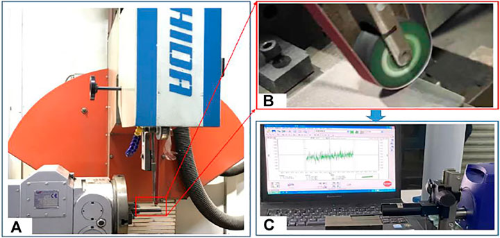
FIGURE 4. Experimental equipment and testing equipment. (A) Seven-axis six-linkage CNC belt grinding machine. (B) Abrasive belt grinding process. (C) Roughness detection of superalloy.
In order to select the corresponding parameter range, exploratory experiments were carried out in the early stage of the experiment, and the corresponding smaller grinding parameters and larger grinding parameters were selected for the experiment. When the grinding parameters are too small, there are empty grinding and owe grinding on the grinding surface, as shown in Figure 5A. When the grinding parameters are too large, there are surface defects and surface burns on the machined surface, as shown in Figure 5B. In order to ensure the integrity of the processing surface and improve the accuracy of the algorithm application, the parameters of the experiment are specified. The linear belt velocity is 12–26 m/s, the feed velocity is distributed in the range of 0.01–0.05 m/min, the grinding pressure is distributed in the range of 10–30 N, and the grinding depth is distributed in the range of 0.2–1 mm.
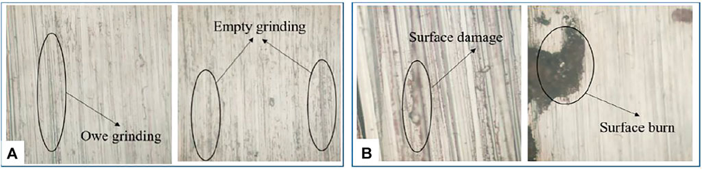
FIGURE 5. Experimental equipment and testing equipment. (A) Machined surface with small grinding parameters. (B) Machined surface with grinding parameters.
The predicted surface roughness under different models is obtained by MATLAB simulation. The predicted value calculated by the algorithm is compared with the parameter value used in the experiment, and the error of the experiment is analyzed, as shown in Figure 6.
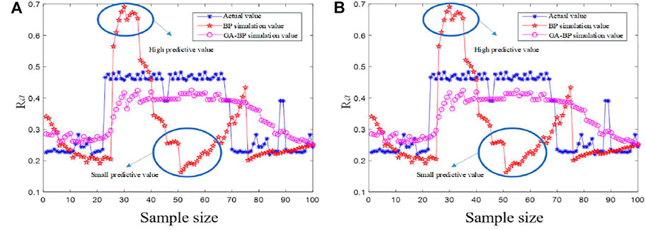
FIGURE 6. Comparison of actual roughness and roughness predicted by different algorithms. (A) BP and GA-BP prediction results analysis. (B) BP and PSO-BP prediction results analysis.
Comparing the prediction results of surface roughness by the BP algorithm, PSO-BP algorithm, and GA-BP algorithm, the results show that the predicted value of the BP algorithm is quite different from the actual value. The error value of the prediction effect is large, the precision is relatively low, and the local prediction value is different. The expected values of the GA-BP and PSO-BP algorithms are in good agreement with the actual values (Figure 6). The mean absolute error (MAE) is introduced to evaluate the algorithm’s stability, and the mean error value of different algorithms is tested according to the absolute error theory (Manuela et al., 2021). The MAEs of the BP, GA-BP, and PSO-BP algorithms are 0.120, 0.085, and 0.079, respectively. It can be known from the above analysis that the MAE value of the PSO-BP algorithm is relatively small, and the algorithm has better prediction results and higher accuracy. By comparing the effects of different algorithms, the expected value and actual value of the expected result of the PSO-BP algorithm have a minor error and a great fit.
GA and PSO are both bionic intelligent algorithms and have good effects on local optimal solutions. The principle of the bionic algorithm is to search for high-performance parts in the solution space and assign better values to greater weights. The optimization algorithm can effectively avoid local optimization, so the prediction effect is better than the BP algorithm. It can be known that all the particles generated in the PSO algorithm have better memory and can well inherit the training results. But the memory in the GA algorithm is not so good, because the related memory will be destroyed during the training process, and the genetic performance is relatively poor. Therefore, the theoretical prediction result of PSO-BP is better than that of GA-BP.
The error values of the BP algorithm, the GA-BP algorithm, and the PSO-BP algorithm are drawn into an error curve (Figure 7). The error generated by the BP algorithm is relatively large. Compared with the BP algorithm, the GA-BP and PSO-BP algorithms have smaller errors, which also proves that the bionic algorithm has optimized the BP algorithm to a certain extent. Error autocorrelation function and partial correlation function are introduced to measure the quality of the algorithm.
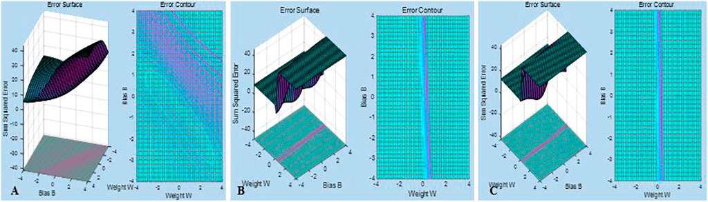
FIGURE 7. Error surface diagram of different optimization methods’ error. (A) Standard BP neural network error surface. (B) GA-BP neural network error surface. (C) PSO-BP neural network error surface.
Figure 8A is the error autocorrelation graph and partial correlation graph predicted by the BP algorithm. In the autocorrelation graph, it can be known that the correlation coefficient value is located on the zero axes for a long time to have a monotonic trend and a normal distribution. It does not have a periodic change trend. It is a non-stationary sequence, indicating that the possibility of autocorrelation is very high. So in the prediction process, the error generated is random and uncontrollable. Simultaneously, the partial correlation graph of samples can know the tailing structure, and some error values exceed the confidence interval. The standard BP neural network algorithm is not so useful for the prediction of the multivariate input model.
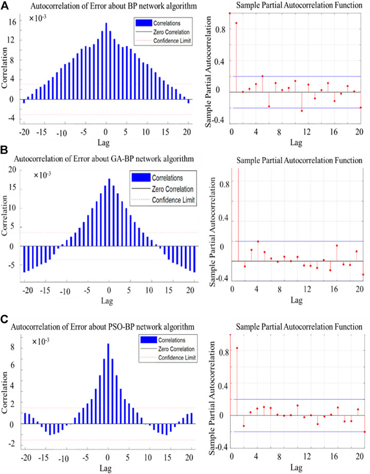
FIGURE 8. Autocorrelation and partial correlation of prediction errors of different algorithms. (A) Autocorrelation and partial correlation of standard BP neural network. (B) Autocorrelation and partial correlation of GA-BP neural network. (C) Autocorrelation and partial correlation of PSO-BP neural network.
Figure 8B is the error autocorrelation graph and partial correlation graph obtained by the GA-BP algorithm. It can be seen that the error autocorrelation graph of the optimized algorithm presents apparent sinusoidal fluctuations, and the autocorrelation coefficient is evenly distributed between positive and negative values. There is individual volatility, indicating that the error fluctuates around a specific value. It can be known that the error value is within a certain range and is controllable. Simultaneously, commemorating the partial correlation diagram of samples can know the tailing structure. All the values do not exceed the confidence interval, indicating that the roughness prediction algorithm has a better prediction effect.
Figure 8C is the error autocorrelation and partial correlation diagram of the PSO-BP algorithm. It can be seen that the algorithm has apparent sinusoidal fluctuations. The autocorrelation value is relatively small (less than the value produced by GA-BP), and there is large volatility, indicating that the error is around a certain one. The value fluctuates, showing that the predicted error value fluctuates within a specific range. The amplitude of the fluctuation is relatively small. Simultaneously, we can know the tailing structure by observing the partial correlation diagram of the samples. All the values do not exceed the confidence interval, indicating that the PSO-BP prediction algorithm’s prediction effect is better than the GA-BP prediction algorithm’s.
The algorithm iteration process of the BP algorithm, GA-BP algorithm, and PSO-BP algorithm is shown (Figure 9). The green, red, and blue lines represent the iterative process graphs for the validation set, test set, and training set, respectively. The BP algorithm meets the requirements of the 32nd generation iteration and is within the error requirements, but after the iteration, the error between the three lines is still relatively large, and the convergence performance is poor. It can be explained that there is an overfitting phenomenon, and the prediction model is not stable. The training results of the GA-BP neural network algorithm meet the requirements of the 13th generation. In the subsequent 6 iterations, the gap is small and the prediction model is very stable, effectively avoiding the phenomenon of overfitting. The predictions work well. Iterative flowchart of the PSO-BP algorithm. The training value can meet the requirements before and after the 31st generation, and the experimental data can also achieve sufficient training, and the error value is relatively small in the subsequent 6 iterations. The mean square error is introduced to measure the stability of different algorithms. After calculation, the MSE values of BP, GA-BP, and PSO-BP algorithms are 0.0213, 0.099, and 0.098, respectively. Therefore, the dataset in the PSO-BP algorithm can be fully trained to avoid overfitting imagination and have better prediction results.
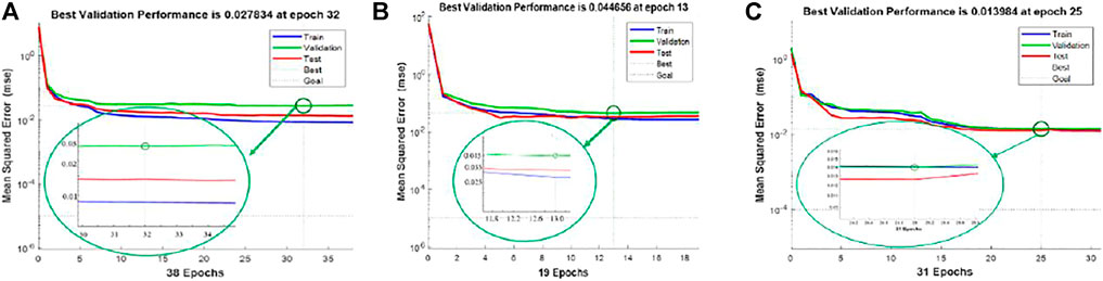
FIGURE 9. Training results of different algorithms. (A) Training result of the BP neural network algorithm. (B) Training result of the GA-BP neural network algorithm. (C) Training result of the PSO-BP neural network algorithm.
To further evaluate the algorithm, the relationship between the training parameters and the number of iterations is plotted (Figure 10). It can be observed that the BP algorithm reaches a minimum value at the 26th iteration and does not change for 6 consecutive iterations. The GA-BP algorithm shows that the optimal solution can be reached when the number of iterations is 13, but a local optimal solution will appear during the training process. The PSO-BP algorithm shows that the optimal solution is obtained after 31 iterations, and there are also some optimal solutions.
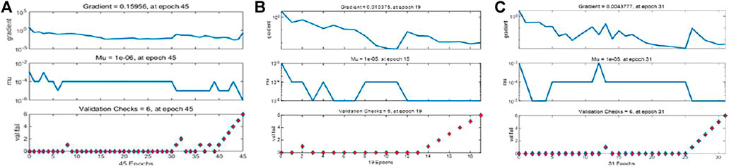
FIGURE 10. Relation diagram of training parameters and iteration times. (A) Relation of BP neural network algorithm. (B) Relation of GA-BP neural network algorithm. (C) Relation of PSO-BP neural network algorithm.
A simple regression analysis was used to evaluate the network training. The closer the R value was to 1 in the regression analysis, the better the effect of the algorithm. The regression analysis of the BP algorithm, the GA-BP algorithm, and the PSO-BP algorithm was carried out (Figure 11). During the training process of the standard BP neural network, the overall fitting value R was 0.946, the overall fitting degree of the GA-BP algorithm was 0.990, and the GA- The overall fitting degree of the BP algorithm is 0.994, and the results show that the PSO-BP algorithm has a good fitting effect.
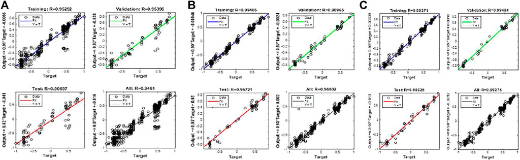
FIGURE 11. Schematic diagram of fitting of different prediction models. (A) Fitting diagram of BP. (B) Fitting diagram of GA-BP. (C) Fitting diagram of PSO-BP.
In this study, a data-driven surface roughness prediction model is proposed. The mapping relationship between processing parameters and surface roughness is established, which avoids the shortcomings of traditional models such as large interference and weak generalization ability and has a broader application prospect. The main conclusions of the article are as follows:
First, based on the BP algorithm model, GA and PSO algorithms are used to optimize the weights and thresholds of the network topology. A surface roughness prediction model for the belt grinding of the GH4169 superalloy is constructed.
Second, the simulation and comparison of BP, GA-BP, and PSO-BP algorithms are conducted by using experimental data as input. The expected values of the different algorithms are compared, which are 0.120, 0.085, and 0.079, respectively. The analysis shows that the prediction accuracy of the PSO-BP algorithm is higher, and it is more suitable for surface roughness prediction in belt grinding of GH4169 superalloy.
Finally, the pros and cons of the proposed algorithm are further analyzed, the error surface graphs of different algorithms are established, and the prediction errors are analyzed. The training process of the algorithm before and after optimization is also analyzed, and the PSO-BP algorithm can fully train the experimental parameters. In addition, the fitting degree of different algorithms is also analyzed in-depth, and the fitting degree of the PSO-BP algorithm can reach 0.993. It shows that the proposed algorithm is more applicable to the grinding of GH4169 superalloy.
However, the exploration of the algorithm principle in this study is relatively simple, and the improvement of the accuracy of the algorithm needs to be further improved. The amount of data in this study is still relatively small, and the training of the model needs to be further improved. For future research, a predictive model for multi-information fusion of multi-sensor inputs can be constructed.
The original contributions presented in the study are included in the article/Supplementary Material; further inquiries can be directed to the corresponding author.
GX, YH, and WL conceived and designed the study. YZ, HG, and BZ performed the experiments. WL and YZ wrote the manuscript. GX and YH reviewed and edited the manuscript. All authors read and approved the manuscript.
This work was supported by the National Natural Science Foundation of China (Grant No. 52175377), the National Science and Technology Major Project (Grant No. 2017-VII-0002-0095), and the National Natural Science Foundation of China (U1908232) (Grant No. CYB20009).
The authors declare that the research was conducted in the absence of any commercial or financial relationships that could be construed as a potential conflict of interest.
The reviewer LW declared a shared affiliation with the author GX to the handling editor at the time of review.
All claims expressed in this article are solely those of the authors and do not necessarily represent those of their affiliated organizations, or those of the publisher, the editors, and the reviewers. Any product that may be evaluated in this article, or claim that may be made by its manufacturer, is not guaranteed or endorsed by the publisher.
Alavijeh, M. S., and Amirabadi, H. (2019). Investigation and Optimization of the Internal Cylindrical Surface Lapping Process of 440c Steel. J. Mech. Sci. Technol. 33 (8), 3933–3941. doi:10.1007/s12206-019-0738-7
Cao, H., Zhou, J., Jiang, P., Hon, K. K. B., Yi, H., and Dong, C. (2020). An Integrated Processing Energy Modeling and Optimization of Automated Robotic Polishing System. Robotics and Computer-Integrated Manufacturing 65, 101973. doi:10.1016/j.rcim.2020.101973
Chang, Z., Jia, Q., Xing, Y., and Chen, Y-L. (2019). Optimization of Grinding Efficiency Considering Surface Integrity of Bearing Raceway. SN Appl. Sci. 1 (9-12), 4243–4252. doi:10.1007/s42452-019-0697-8
Cui, B., Sun, F., Ding, Q., Wang, H., Lin, Y., Shen, Y., et al. (2021). Preparation and Characterization of Sodium Aluminum Silicate-Polymer Composites and Effects of Surface Roughness and Scratch Directions on Their Flexural Strengths. Front. Mater. 8, 655156. doi:10.3389/fmats.2021.655156
Ding, Y., He, W-P., Zhang, W., Wang, W., Li, Y-J., and Dong, R. (2010). Tool Life Prediction Model Based on BP Neural Network. Aeronaut. Manuf. Technol. 6 (8), 93–96. doi:10.3969/j.issn.1671-833X.2010.08.019
Galati, M., Rizza, G., Defanti, S., and Denti, L. (2021). Surface Roughness Prediction Model for Electron Beam Melting (EBM) Processing Ti6Al4V. Precision Eng. 69 (2), 19–28. doi:10.1016/j.precisioneng.2021.01.002
Golbabai, A., and Mohebianfar, E. (2017). A New Method for Evaluating Options Based on Multiquadric RBF-FD Method. Appl. Mathematics Comput. 308, 130–141. doi:10.1016/j.amc.2017.03.019
Gao, H., Yang, Y., Xu, Q.-H., Wang, J.-L., and Wang, Y. (2021). Experimental Study on High Efficiency Grinding Process of 5G Copper Clad Laminate Composites. Diam. Abrasives. Eng. 41, 82–88. doi:10.13394/j.cnki.jgszz.2021.3.0012
Gu, Q., Deng, Z., Lv, L., Liu, T., Teng, H., Wang, D., et al. (2021). Prediction Research for Surface Topography of Internal Grinding Based on Mechanism and Data Model. Int. J. Adv. Manuf Technol. 113 (3), 821–836. doi:10.1007/s00170-021-06604-7
Guo, W., Wu, C., Ding, Z., and Zhou, Q. (2021). Prediction of Surface Roughness Based on A Hybrid Feature Selection Method and Long Short-Term Memory Network in Grinding. Int. J. Adv. Manuf Technol. 112 (9), 2853–2871. doi:10.1007/s00170-020-06523-z
Huang, Y., He, S., Xiao, G., Li, W., Jiahua, S., and Wang, W. (2020). Effects Research on Theoretical-Modelling Based Suppression of the Contact Flutter in Blisk Belt Grinding. J. Manufacturing Process. 54, 309–317. doi:10.1016/j.jmapro.2020.03.021
Huang, Y., Xiao, G-J., and Zou, L. (2016). Current Situation and Development Trend of Polishing Technology for Blisk. Chin. J. Aeronaut. 37 (7), 2045–2064. doi:10.7527/S1000-6893.2016.0055
Huang, Y., Xiao, G., Zhao, H., Zou, L., Zhao, L., Liu, Y., et al. (2018). Residual Stress of Belt Polishing for the Micro-stiffener Surface on the Titanium Alloys. Proced. CIRP 71, 11–15. doi:10.1016/j.procir.2018.05.007
Klocke, F., Gierlings, S., Brockmann, M., and Veselovac, D. (2014). Force-Based Temperature Modeling for Surface Integrity Prediction in Broaching Nickel-Based Alloys. Proced. CIRP 13, 314–319. doi:10.1016/j.procir.2014.04.053
Li, C., Piao, Y., Meng, B., Hu, Y., Li, L., and Zhang, F. (2022). Phase Transition and Plastic Deformation Mechanisms Induced by Self-Rotating Grinding of GaN Single Crystals. Int. J. Mach. Tools Manuf. 172, 103827. doi:10.1016/j.ijmachtools.2021.103827
Pandiyan, V., Caesarendra, W., Tjahjowidodo, T., and Tan, H. H. (2018). In-Process Tool Condition Monitoring in Compliant Abrasive Belt Grinding Process Using Support Vector Machine and Genetic Algorithm. J. Manufacturing Process. 31, 199–213. doi:10.1016/j.jmapro.2017.11.014
Slătineanu, L., Coteaţă, M., Dodun, O., Iosub, A., and Sîrbu, V. (2010). Some Considerations Regarding Finishing by Abrasive Flap Wheels. Int. J. Mater. Form. 3 (2), 123–134. doi:10.1007/s12289-009-0665-8
Wang, X., Xu, C-L., Li, Z-X., Pei, C-H., and Tang, Z-H. (2020). Effect of Shot Peening Intensity and Surface Coverage on Room-Temperature Fatigue Property of TC4 Titanium Alloy. Cailiao. Gongcheng. 48 (9), 138–143. doi:10.11868/j.issn.1001-4381.2019.000142
Wu, D-H. (2007). A Prediction Model for Surface Roughness in Milling Based on Least Square Support Vector Machine. Chin. J. Mech. Eng-en. 18 (07), 838–841. doi:10.3321/j.issn:1004-132X.2007.07.020
Xiao, G., Chen, B., Li, S., and Zhuo, X. (2022). Fatigue Life Analysis of Aero-Engine Blades for Abrasive Belt Grinding Considering Residual Stress. Eng. Fail. Anal. 131, 105846–10584614. doi:10.1016/j.engfailanal.2021.105846
Xiao, G., and Huang, Y. (2019). Micro-Stiffener Surface Characteristics with Belt Polishing Processing for Titanium Alloys. Int. J. Adv. Manuf Technol. 100 (1-4), 349–359. doi:10.1007/s00170-018-2727-x
Xiao, G., Zhang, Y-D., Huang, Y., Zhang, Y., Huang, Y., Song, S., et al. (2021). Grinding Mechanism of Titanium alloy: Research Status and prospect. J. Adv. Manuf. Sci. Tech. 1 (1), 2020001–2020012. doi:10.51393/j.jamst.2020001
Xu, L., Huang, C., Li, C., Wang, J., Liu, H., and Wang, X. (2020). An Improved Case Based Reasoning Method and its Application in Estimation of Surface Quality toward Intelligent Machining. J. Intell. Manuf. 32 (1), 313–327. doi:10.1007/s10845-020-01573-2
Zhang, M-J., Wang, C., and Chen, H. (2012). The Application Research on the Combination of IMF Energy and RBF Neural Network in Rolling Bearing Fault Diagnosis. Machinery 39 (06), 63–66+70. doi:10.3969/j.issn.1006-0316.2012.06.017
Zhang, S., Yang, Z., Jiang, R., Jin, Q., Zhang, Q., and Wang, W. (2021). Effect of Creep Feed Grinding on Surface Integrity and Fatigue Life of Ni3al Based Superalloy IC10. Chin. J. Aeronautics 34 (1), 438–448. doi:10.1016/j.cja.2020.02.025
Zhou, K., Xu, J., Xiao, G., and Huang, Y. (2022). A Novel Low-Damage and Low-Abrasive Wear Processing Method of Cf/Sic Ceramic Matrix Composites: Laser-Induced Ablation-Assisted Grinding. J. Mater. Process. Technology 302, 117503. doi:10.1016/j.jmatprotec.2022.117503
Keywords: belt grinding, GH4169 superalloy, roughness prediction, data driven, intelligent algorithm
Citation: Zhang Y, Xiao G, Gao H, Zhu B, Huang Y and Li W (2022) Roughness Prediction and Performance Analysis of Data-Driven Superalloy Belt Grinding. Front. Mater. 9:765401. doi: 10.3389/fmats.2022.765401
Received: 27 August 2021; Accepted: 28 March 2022;
Published: 13 May 2022.
Edited by:
Tadeusz Hryniewicz, Koszalin University of Technology, PolandReviewed by:
Liang Wu, Chongqing University, ChinaCopyright © 2022 Zhang, Xiao, Gao, Zhu, Huang and Li. This is an open-access article distributed under the terms of the Creative Commons Attribution License (CC BY). The use, distribution or reproduction in other forums is permitted, provided the original author(s) and the copyright owner(s) are credited and that the original publication in this journal is cited, in accordance with accepted academic practice. No use, distribution or reproduction is permitted which does not comply with these terms.
*Correspondence: Guijian Xiao, eGlhb2d1aWppYW5AY3F1LmVkdS5jbg==
Disclaimer: All claims expressed in this article are solely those of the authors and do not necessarily represent those of their affiliated organizations, or those of the publisher, the editors and the reviewers. Any product that may be evaluated in this article or claim that may be made by its manufacturer is not guaranteed or endorsed by the publisher.
Research integrity at Frontiers
Learn more about the work of our research integrity team to safeguard the quality of each article we publish.