Aluminum electron energy loss spectra. A comparison between Monte Carlo and experimental data

One of the most interesting applications of the Monte Carlo method consists in the simulation of the energy loss spectrum of backscattered electrons when a solid target is bombarded with an electron beam of given kinetic energy. Knowing the elastic and inelastic scattering cross-sections of the electrons in their interaction with the atoms of the target, it is possible to calculate the probabilities of angular diffusion and the loss of kinetic energy for each collision between the electrons of the incident beam and the atoms of the target. In this way, it is possible to model the history of each electron following its trajectory and calculating its energy losses, its final energy, and the exit point from the target surface whether and where it exists. By averaging over a large number of trajectories, it is possible to obtain a spectrum representing the energy distribution of the backscattered electrons from any given solid target. This paper compares experimental and Monte Carlo data concerning reflection electron energy loss spectra. In particular, the paper is aimed at understanding the interplay between surface and bulk features for incident electrons in Al.

1 Introduction

The Monte Carlo strategy is the best approach in the investigation of radiation effects on matter. It requires an accurate calculation of its main ingredients, i.e., the inelastic and the elastic scattering probabilities (Shimizu and Ding, 1992; Joy, 1995; Dapor, 2003; Dapor, 2017; Dapor, 2020).

Inelastic collisions are adequately taken into account by the evaluation of the differential inverse inelastic mean free path, which enables the accurate description of the statistical fluctuations of the energy losses (the so-called energy straggling). In dielectric theory, this quantity can be computed once the energy loss function is known (Ritchie, 1957; Mermin, 1970; Ritchie and Howie, 1977; Penn, 1987; Tanuma et al., 1988; Ashley, 1990; Abril et al., 1998; Tanuma et al., 2004; Denton et al., 2008; Bourke and Chantler, 2012; Dapor, 2015; de Vera and Garcia-Molina, 2019).

Elastic collisions, on the other hand, can be described by the numerical solution of the quantum-relativistic equations governing the electron interactions with a screened central potential (relativistic partial wave expansion method) (Mott, 1929; Riley et al., 1975; Kessler, 1985; Jablonski, 1991; Salvat and Mayol, 1993; Burke and Joachain, 1995; Dapor, 1995a; Dapor, 1995b; Dapor, 1996; Mayol and Salvat, 1997; Salvat, 2003; Jablonski et al., 2004; Salvat et al., 2005; Dapor, 2022a; Dapor, 2022b).

After explaining how to calculate these two important quantities, we describe their inclusion in a Monte Carlo program that takes into account both bulk and surface features.

The aim of this work is to perform Monte Carlo simulations of REEL spectra in the primary electron energy range from 1,000 eV to 10,000 eV in order to investigate the interaction between surface and bulk characteristics when electrons impinge on solid targets. Al is used as a case study.

Monte Carlo simulations are compared to experimental REEL spectra excited by 1,000 eV and 2,000 eV electrons in Al.

The REEL spectra concern energy losses of incident beam electrons as a result of inelastic interactions with the target’s atoms.

In the field of electron microscopy, secondary electrons are also very important. The secondary electrons, not dealt with in this work, are the result of the cascade of electrons produced by the ionizations of the target atoms.

The Monte Carlo method allows simulation of the entire secondary electron cascade and calculation of the secondary and total emission yield, very important quantities for aiding the analysis of secondary electron images. The present Monte Carlo code was indeed also used for simulating both the energy distribution of the secondary electrons and the secondary and total electron yields, by following the whole cascade of secondary electrons (see, for example, Refs. (Dapor, 2017; Dapor, 2020)). The study of secondary electrons also involves electron-phonon interaction, i.e., temperature effects (Dapor, 2020).

However, secondary electrons are not relevant for the present study, as here we are interested in electrons emerging from the target with energies higher than 900 eV, while secondary electrons emerge with typical energies smaller than 50 eV.

2 Theory

2.1 Inelastic processes

2.1.1 The original Drude–Lorentz theory

Let us consider an elastically bound electron, with elastic constant $m{\omega }_0^2$, natural frequency ω₀, and subject to a frictional damping effect described by the damping constant γ₀ (which is the reciprocal of the relaxation time τ₀). The electron displacement r satisfies the equation

$\frac{d^2\mathbf{r}}{d{t}^2}+{\gamma }_0\frac{d\mathbf{r}}{dt}+{\omega }_0^2\mathbf{r}=\frac{e}{m}\mathbf{E},(1)$

where

$\mathbf{E}={\mathbf{E}}_0\exp \left(i\omega t\right),(2)$

is the electric field, e is the electron charge, m is the electron mass, and ω is the oscillation frequency. We look for stationary solutions having the form

$\mathbf{r}={\mathbf{r}}_0\exp \left(i\omega t\right).(3)$

If n is the number of outer-shell electrons per unit volume in the solid, then the dielectric polarization density P of the material is given by

$\mathbf{P}=en\mathbf{r}.(4)$

On the other hand,

$\mathbf{P}=\chi \mathbf{E},(5)$

where χ is the electric susceptibility

$\chi =\frac{\epsilon -1}{4\pi }.(6)$

Here ɛ = ɛ(ω) is the dielectric function, so that the electric displacement D is given by

$\mathbf{D}=\mathbf{E}+4\pi \mathbf{P}=\left(1+4\pi \chi \right)\mathbf{E}=\epsilon \mathbf{E}.(7)$

Since

$\mathbf{E}=\frac{\mathbf{P}}{\chi }=\frac{4\pi en}{\epsilon -1}\mathbf{r}=\frac{4\pi en}{\epsilon -1}{\mathbf{r}}_0\exp \left(i\omega t\right),(8)$

we obtain

$-{\omega }^2-i\omega {\gamma }_0+{\omega }_0^2=\frac{4\pi e^{2}n/m}{\epsilon -1}.(9)$

As a consequence

$\epsilon \left(\omega \right)=1-\frac{4\pi e^{2}n}{m}\frac{1}{{\omega }^2-{\omega }_0^2-i\omega {\gamma }_0}.(10)$

In the case of a superimposition of bound oscillators, the dielectric function can be written as:

$\epsilon \left(\omega \right)=1-\frac{4\pi e^{2}N{Z}_{\mathrm{V}}}{m}\sum _j\frac{f_j}{{\omega }^2-{\omega }_j^2-i\omega {\gamma }_j}.(11)$

where N is the number of atoms per unit volume in the target, Z_V the number of outer-shell electrons (n = NZ_V), γ_j are positive frictional damping coefficients, and f_j = Z_j/Z_V are the fractions of the electrons involved in the excitation and bound with energies ω_j, so that

$\sum _j{f}_j=1.(12)$

In the general case of the presence of free and bound electrons, if f₀ is the fraction of free electrons so that ω₀ = 0, we have

$\begin{array}{ll}\hfill \epsilon \left(\omega \right)& =1-\frac{4\pi e^{2}N{Z}_{\mathrm{V}}}{m}\frac{f_0}{{\omega }^2-i\omega {\gamma }_0}\hfill \\ \hfill & -\frac{4\pi e^{2}N{Z}_{\mathrm{V}}}{m}\sum _j\frac{f_j}{{\omega }^2-{\omega }_j^2-i\omega {\gamma }_j}.\hfill \end{array}(13)$

Up to now, we were interested only in the optical response due to the outer-shell electrons, so the total number of electrons involved in the excitation was the number of outer-shell electrons. The last term in the last equation then represents, according to Yubero and Tougaard (1992), the contribution of the interband transitions with energy ℏω_j, oscillator strength f_j, and lifetime ${\gamma }_j^{-1}$.

Neglecting interband transitions due to the bond electrons, so that f₀ = 1 and f_j = 0 ∀j ≠ 0, the above equation becomes

$\epsilon \left(\omega \right)=1-\frac{{\omega }_p^2}{{\omega }^2-i\omega {\gamma }_0}(14)$

where

${\omega }_p=\sqrt{\frac{4\pi e^{2}N{Z}_{\mathrm{V}}}{m}}=\sqrt{\frac{4\pi e^{2}n}{m}}(15)$

is the plasma frequency of the outer-shell electrons. The real part ɛ₁(ω) and the imaginary part ɛ₂(ω) of ɛ(ω) are given, in this case, respectively by

${\epsilon }_1\left(\omega \right)=1-\frac{{\omega }_p^2}{{\omega }^2+{\gamma }_0^2},(16)$

${\epsilon }_2\left(\omega \right)=-\frac{{\gamma }_0}{\omega }\frac{{\omega }_p^2}{{\omega }^2+{\gamma }_0^2}.(17)$

Please note that ɛ₁(ω) is equal to 0 when the frequency satisfies the equation:

${\omega }^2={\omega }_p^2-{\gamma }_0^2.(18)$

So, if we can neglect the frictional damping, i.e., if ${\omega }_p^2\gg {\gamma }_0^2$, the real part of the dielectric function is zero when the frequency is approximately equal to the plasma frequency.

2.1.2 Outer-shell and core electrons in Al

In the original Drude–Lorentz theory, we were interested in the optical response due to the outer-shell electrons only. On the other hand, when the frequency becomes high enough, core electrons become involved in the excitation as well, so the total number of electrons involved in the excitation is the atomic number Z. For Al, neglecting interband transitions and indicating with Z_L the number of electrons in the L − shell and with Z_K the number of electrons in the K − shell, we can write

$\begin{array}{ll}\hfill \epsilon \left(\omega \right)& =1-{\mathrm{\Omega }}_p^{2}Z\left[\frac{Z_{\mathrm{V}}/Z}{{\omega }^2-i\omega {\gamma }_{\mathrm{V}}}\right.\hfill \\ \hfill & +\left.\frac{Z_{\mathrm{L}}/Z}{{\omega }^2-{\omega }_{\mathrm{L}}^2-i\omega {\gamma }_{\mathrm{L}}}+\frac{Z_{\mathrm{K}}/Z}{{\omega }^2-{\omega }_{\mathrm{K}}^2-i\omega {\gamma }_{\mathrm{K}}}\right]\hfill \end{array}(19)$

where

$\hslash {\mathrm{\Omega }}_p=\sqrt{\frac{4\pi N{\hslash }^2{e}^2}{m}}=\sqrt{4\pi N{e}^4{a}_0}=9.13\mathrm{e}\mathrm{V}.(20)$

Please note that, for Al, N = 6.04 × 10²² atoms per cm³, Z = 13, Z_V = 3, Z_L = 8, Z_K = 2, ℏω_L = 130.62 eV, ℏω_K = 1,569.56 eV, ℏγ_V = 1.5 eV, ℏγ_L = 99.6 eV, and ℏγ_K = 1,116 eV. Please also note that the plasma energy due to the outer-shell electrons only, ℏω_p, is given by

$\hslash {\omega }_p=\hslash {\mathrm{\Omega }}_p\sqrt{Z_{\mathrm{V}}}=15.8\mathrm{e}\mathrm{V},(21)$

so that a bulk plasmon is expected to be found at 15.8 eV from the elastic peak in the reflection electron energy loss spectrum.

2.1.3 Energy loss function and sum rules

The energy loss function (ELF) is defined as the reciprocal of the imaginary part of the dielectric function (Ritchie, 1957). Since

$\epsilon \left(\omega \right)={\epsilon }_1\left(\omega \right)+i{\epsilon }_2\left(\omega \right),(22)$

in the optical limit (no momentum transfer) the ELF is thus defined as ¹

$f\left(\omega \right)=\mathrm{I}\mathrm{m}\left[\frac{1}{\epsilon \left(\omega \right)}\right]=-\frac{{ϵ}_2\left(\omega \right)}{{ϵ}_1^2\left(\omega \right)+{ϵ}_2^2\left(\omega \right)}(28)$

From Eq. 28 it is clear that a maximum of the ELF is obtained when the real part ϵ₁(ω) of the dielectric function is equal to 0. This resonance (assuming that the frictional damping effect can be neglected) occurs when the frequency is equal to the plasma frequency. In Figure 1 we have represented the calculated ELF of Al compared to the Henke et al. experimental optical data (Henke et al., 1993).

FIGURE 1

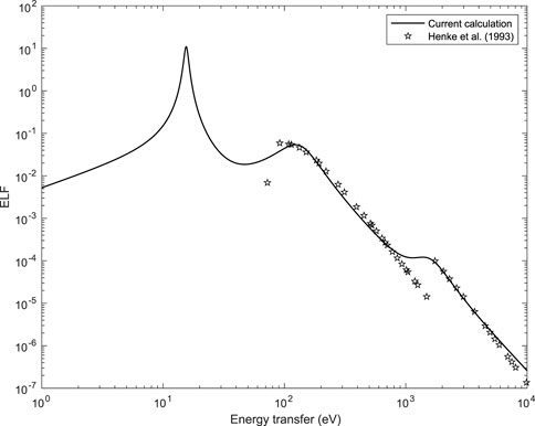
FIGURE 1. Long wavelength limit (k →0) of the ELF of Al (solid line) compared to experimental optical data from Ref. (Henke et al., 1993) (symbols). The dielectric function was calculated using Eqs 19, 20, 28 with N =6.04×10²² atoms per cm³, Z =13, Z_V =3, Z_L =8, Z_K =2, ℏω_L =130.62 eV, ℏω_K =1,569.56 eV, ℏγ_V = 1.5 eV, ℏγ_L = 99.6 eV, and ℏγ_K = 1,116 eV.

The ELF must satisfy the ps-sum rule (perfect screening sum rule). If

$-\frac{2}{\pi }{\int }_0^{{\omega }_{\text{max}}}\frac{1}{\omega }\mathrm{I}\mathrm{m}\left[\frac{1}{\epsilon \left(\omega \right)}\right]=P_{\text{eff}}\left({\omega }_{\text{max}}\right),(29)$

then

$\underset{{\omega }_{\text{max}}\to \infty }{\lim }{P}_{\text{eff}}\left({\omega }_{\text{max}}\right)=1.(30)$

P_eff was represented as a function of ℏω_max in Figure 2.

FIGURE 2

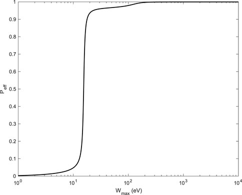
FIGURE 2. Plot of P_eff of Al as a function of W_max = ℏω_max. See Eq. 29. When W_max →∞, P_eff →1

The f-sum rule must also be satisfied. If

$-\frac{2}{\pi {\mathrm{\Omega }}_p^2}{\int }_0^{{\omega }_{\text{max}}}\omega \mathrm{I}\mathrm{m}\left[\frac{1}{\epsilon \left(\omega \right)}\right]=Z_{\text{eff}}\left({\omega }_{\text{max}}\right),(31)$

then

$\underset{{\omega }_{\text{max}}\to \infty }{\lim }{Z}_{\text{eff}}\left({\omega }_{\text{max}}\right)=Z.(32)$

Z_eff was represented as a function of ℏω_max in Figure 3, where contributions of valence, L-shell, and K-shell electrons were highlighted.

FIGURE 3

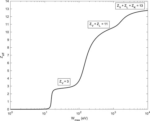
FIGURE 3. Plot of the effective atomic number Z_eff of Al as a function of W_max = ℏω_max. See Eq. 31. When W_max →∞, Z_eff → Z. Contributions of valence, L-shell, and K-shell electrons are pointed out.

2.1.4 Beyond the optical limit

Up to now, we have dealt with the approximation of the dielectric function without k dependence (optical limit). According to Yubero and Tougaard (1992), the k dependence of the dielectric function can be described by the use of the following approximation:

$\begin{array}{ll}\hfill \epsilon \left(k,\omega \right)& =1-{\mathrm{\Omega }}_p^2\left[\frac{Z_{\mathrm{V}}}{{\omega }^2-{\omega }_k^2-i{\gamma }_{\mathrm{V}}\omega }\right.\hfill \\ \hfill & +\left.\frac{Z_{\mathrm{L}}}{{\omega }^2-{\omega }_k^2-{\omega }_{\mathrm{L}}^2-i{\gamma }_{\mathrm{L}}\omega }+\frac{Z_{\mathrm{K}}}{{\omega }^2-{\omega }_k^2-{\omega }_{\mathrm{K}}^2-i{\gamma }_{\mathrm{K}}\omega }\right],\hfill \end{array}(33)$

where

$\hslash {\omega }_k=\frac{{\hslash }^2{k}^2}{2m},(34)$

so that the energy loss function itself is a function of both the energy loss ℏω and the momentum transfer ℏk according to the equation:

$f\left(k,\omega \right)=\mathrm{I}\mathrm{m}\left[\frac{1}{\epsilon \left(k,\omega \right)}\right].(35)$

The dispersion law represented by Eq. 34 satisfies the so-called Bethe ridge which establishes that, when k → ∞, ℏω_k should approach $\frac{{\hslash }^2{k}^2}{2m}$. Actually, Eq. 34 is valid for high momentum transfer. According to (Ritchie, 1957) and (Ritchie and Howie, 1977), the following dispersion law should be used

${\hslash }^2{\omega }_k^2=\frac{12E_{\mathrm{F}}}{5}\frac{{\hslash }^2{k}^2}{2m}+{\left(\frac{{\hslash }^2{k}^2}{2m}\right)}^2,(36)$

where E_F is the Fermi energy (E_F = 11.7 eV for Al (Ashcroft and Mermin, 1976)). This is the most general equation satisfying the constraint represented by the Bethe ridge that can be obtained within the so-called Random Phase Approximation (RPS) for a 3D electron gas. For intermediate values of k, the term $\frac{12E_{\mathrm{F}}}{5}\frac{{\hslash }^2{k}^2}{2m}$ in the dispersion law, Eq. 36, cannot be ignored. Please note that the Mermin dielectric function (Mermin, 1970) includes naturally the k dependence of ɛ without the necessity to introduce a dispersion law (Abril et al., 1998). As discussed in (Dapor, 2015), due to the quite large uncertainty in the experimental data, it is not always clear which theory provides results in better agreement with the experiment. Actually, both Mermin and Drude–Lorentz approaches seem to be compatible with the available experimental data about the inelastic mean free path. Even if the Mermin theory is more complete, the Drude–Lorentz theory is often used, for practical purposes, due to its great simplicity.

2.1.5 Differential inverse inelastic mean free path

Equation 35 allows calculating, according to Ritchie’s theory (Ritchie, 1957), the double differential inverse inelastic mean free path

$\frac{d^2{\lambda }_{\text{inel}}^{-1}}{d\hslash \omega d\hslash k}=\frac{1}{\pi a_{0}E}\frac{1}{\hslash k}f\left(k,\omega \right),(37)$

where E is the kinetic energy of the incident electron and a₀ is the Bohr radius. From conservation laws it follows that the minimum value ℏk_min and the maximum value ℏk_max of the momentum transfer ℏk are given, respectively, by

$\hslash k_{\text{min}}=\sqrt{2mE}-\sqrt{2m\left(E-\hslash \omega \right)},(38)$

$\hslash k_{\text{max}}=\sqrt{2mE}+\sqrt{2m\left(E-\hslash \omega \right)},(39)$

so that we can easily calculate the differential inverse inelastic mean free path as

$\frac{d{\lambda }_{\text{inel}}^{-1}}{d\hslash \omega }=\frac{1}{\pi a_{0}E}{\int }_{k_{\text{min}}}^{k_{\text{max}}}\frac{dk}{k}f\left(k,\omega \right).(40)$

2.1.6 Inelastic mean free path

Once the differential inverse inelastic mean free path is known, the inverse inelastic mean free path for a metal can be calculated by integrating from zero to the maximum energy loss ℏω_max:

${\lambda }_{\text{inel}}^{-1}={\int }_0^{\hslash {\omega }_{\text{max}}}\frac{d{\lambda }_{\text{inel}}^{-1}}{d\hslash \omega }d\hslash \omega .(41)$

Please note that, on the one hand, according to (Denton et al., 2008) the maximum energy loss should be given by

$\hslash {\omega }_{\text{max}}=\min \left(\frac{E}{2},E-E_{\mathrm{F}}\right),(42)$

where the integration limit of E/2 is attributed to the indistinguishability of the incident and the secondary electrons.

On the other hand, according to Bourke and Chantler (2012), when the dominant cause of inelastic losses is represented by plasmon excitations, this integration limit should be instead

$\hslash {\omega }_{\text{max}}=E-E_{\mathrm{F}},(43)$

as a plasmon is a distinct entity, so it is distinguishable from an electron. Please note that de Vera and Garcia-Molina discussed in detail the issue of the integration limits in energy (de Vera and Garcia-Molina, 2019).

Since we are interested in describing plasmon losses, Eq. 43 will be used. The inelastic mean free path calculated using Eqs 41, 43 is compared, in Figure 4, to the calculations by Ashley (1990) and by Tanuma et al. (1988), Tanuma et al. (2004).

FIGURE 4

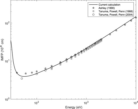
FIGURE 4. Inelastic mean free path of Al (solid line) as a function of the incident electron beam kinetic energy compared to (Ashley, 1990) and (Tanuma et al., 1988; Tanuma et al., 2004) (symbols).

2.1.7 Inelastic cumulative probability

The cumulative probability of inelastic scattering P_inel(W) is a central quantity in Monte Carlo simulations. It is given by

$P_{\text{inel}}\left(W\right)={\lambda }_{\text{inel}}{\int }_0^W\frac{d{\lambda }_{\text{inel}}^{-1}}{d\hslash \omega }d\hslash \omega .(44)$

2.1.8 Surface

Several theories have been developed that allow estimating the surface excitation probability. The so-called surface excitation parameter (SEP) represents the average number of surface excitations an electron experiences crossing the surface once. Knowledge of the SEP allows evaluating the probability P_s of a given number of surface excitations in a surface crossing (Werner et al., 2001). Based on the theoretical work of Tung et al. (1994), Werner et al. (2001) proposed the following formula for the calculation of P_s for an electron crossing the surface with an angle θ with respect to the surface normal:

$P_s\left(\theta ,E\right)=\frac{1}{a\sqrt{E}\cos \theta +1},(45)$

where a is a parameter depending on the material (a ≈ 0.12 for Al). A Monte Carlo simulation using Eq. 45 to deal with surface plasmons was described in Ref. (Dapor et al., 2011).

Dapor et al. (2012) calculated the energy loss spectra of Al and Si under the assumption that experimental spectra arise from electrons undergoing a single large-angle elastic scattering event (so-called V-type trajectories (Jablonski and Powell, 2004)) and describing inelastic scattering by the Chen and Kwei differential inverse inelastic mean free path, dependent on the distance from the surface (in the solid and in the vacuum) and on the angle of surface crossing (Chen and Kwei, 1996). Reasonable agreement was found between these calculations and available experimental data for bulk and surface plasmon peaks in the energy range from 500 eV to 2,000 eV (Dapor et al., 2012).

The surface is an interface between the bulk of the material and the vacuum. Since the dielectric function depends on the material, we expect the mean energy of the plasmons characterizing the surface (surface plasmons) to be different from the mean energy of the bulk plasmons.

Due to the continuity of the electric field at the interface between any two materials a and b, we have (Egerton, 2011)

${\epsilon }_a\left(\omega \right)+{\epsilon }_b\left(\omega \right)=0,(46)$

where ɛ_a(ω) and ɛ_b(ω) are the dielectric functions on either side of the interface, so that, neglecting frictional damping effects, the surface plasmons at the boundary between a metal and vacuum are expected to be observed when the frequency ω = ω_s satisfies the equation

$\left(1-\frac{{\omega }_p^2}{{\omega }_s^2}\right)+1=0.(47)$

Therefore

${\omega }_s^2=\frac{{\omega }_p^2}{2}.(48)$

As a consequence, indicating with E_p = ℏω_p = 15.8 eV the mean bulk plasmon energy of Al, the mean energy of the surface plasmon peaks in the Al REEL spectra should be found at energy $E_s=E_p/\sqrt{2}\approx 11.2$ eV.

Please note the existence of the begrenzungs effect, i.e., a reduction of the intensity of the bulk plasmon due to the boundary, which was discussed by Ritchie (1957). In the limit of large target thickness, Ritchie demonstrated that the total transition probability is given by two terms. The first one is just the target thickness times the transition probability per unit path length in an infinite target. The second one is proportional to

$\mathrm{I}\mathrm{m}\left[-\frac{{\left(1-\epsilon \right)}^2}{\epsilon \left(1+\epsilon \right)}\right]=\mathrm{I}\mathrm{m}\left(\frac{4}{\epsilon +1}-1-\frac{1}{\epsilon }\right).(49)$

The begrenzungs effect is represented by Im [ − 1–1/ɛ] (Egerton, 2011).

Chiarello et al. (1984), observed that the REEL spectrum can be described by the combination of two terms, arising from surface and bulk inelastic scattering. According to the approach of these authors, the bulk and surface excitations can be described by the combined effect of the bulk energy loss function given by Eq. 35 and the surface energy loss function which, according to (Chiarello et al., 1984), (Ohno, 1989), and (Yubero et al., 1990) can be described as

$f_s\left(k,\omega \right)=\mathrm{I}\mathrm{m}\left[\frac{1}{\epsilon \left(k,\omega \right)+1}\right](50)$

Attempts to include in Monte Carlo simulations the combination of surface and bulk energy loss functions, proposed by Chiarello et al. (1984), can be found in Refs. (Calliari et al., 2007; Dapor et al., 2008). With this paper, we are also presenting results obtained using the Chiarello et al. approach. We will show that, compared to the previously quoted investigations (Refs. (Calliari et al., 2007; Dapor et al., 2008)), a better agreement is found for the absolute values of the plasmon peaks. We attribute this observed better agreement to the inclusion of the contribution of the inner shell electrons in the calculation of the dielectric function and thus to a better description of the inelastic mean free path and of the inelastic cumulative probability for energies higher than 1,000 eV. ²

2.2 Elastic processes

2.2.1 Dirac equation in a central field

An electron in a central field is described by the two following equations (Bunyan and Schonfelder, 1965)

$\left[W-V\left(r\right)+1\right]F_l^{\pm }+\frac{d{G}_l^{\pm }}{dr}+\frac{1+k^{\pm }}{r}{G}_l^{\pm }=0,(52)$

$-\left[W-V\left(r\right)-1\right]G_l^{\pm }+\frac{d{F}_l^{\pm }}{dr}+\frac{1-k^{\pm }}{r}{F}_l^{\pm }=0,(53)$

where W and V(r) are the particle energy and the atomic potential energy, respectively, both expressed in units of mc², r is the distance from the atom expressed in ℏ/mc units, m is the electron mass, c is the speed of light, ℏ = h/2π, and h is the Planck’s constant. Here l = 0, 1, 2, … , ∞ and “±” signs refer to the spin: “+” applies to spin up, i.e., j = l + 1/2 while “−” corresponds to spin down, i.e., j = l − 1/2. k⁺ = −(l + 1) while k⁻ = l. Equations 52, 53 represent the Dirac description of an electron in a central potential.

2.2.2 Lin, Sherman, and Percus transformation

With the transformations

$G_l^{\pm }=A_l^{\pm }\frac{\cos {\varphi }_l^{\pm }\left(r\right)}{r}(54)$

$F_l^{\pm }=A_l^{\pm }\frac{\sin {\varphi }_l^{\pm }\left(r\right)}{r}(55)$

the first-order differential equation

$\frac{d{\varphi }_l^{\pm }\left(r\right)}{dr}=\frac{k^{\pm }}{r}\sin \left[2{\varphi }_l^{\pm }\left(r\right)\right]-\cos \left[2{\varphi }_l^{\pm }\left(r\right)\right]+W-V\left(r\right),(56)$

follows from Eqs 52, 53 (Lin et al., 1963).

2.2.3 Electrostatic atomic potential energy

The electrostatic atomic potential energy V(r) can be calculated as the product of the Coulomb potential energy multiplied by a screening function ξ(r) expressed as a superposition of Yukawa functions, given by (Cox and Bonham, 1967; Salvat et al., 1987)

$\xi \left(r\right)=\sum _{i=1}^p{\gamma }_i\exp \left(-{\lambda }_{i}r\right).(57)$

Exchange effects should be included in the calculation of the atomic potential energy. They can be described by using the Furness and McCarthy local approximation (Furness and McCarthy, 1973).

2.2.4 Phase shifts

Equation 56 has to be solved in order to evaluate

${\tilde{\varphi }}_l^{\pm }=\underset{r\to \infty }{\lim }{\varphi }_l^{\pm }.(58)$

Once ${\tilde{\varphi }}_l^{\pm }$ is known, the phase shifts ${\eta }_l^{\pm }$ of the scattered waves in an elastic scattering experiment may be calculated by (Kessler, 1985; Jablonski, 1991; Salvat and Mayol, 1993; Dapor, 1995a; Dapor, 1995b; Burke and Joachain, 1995; Dapor, 1996; Mayol and Salvat, 1997; Salvat, 2003; Salvat et al., 2005; Dapor, 2022a; Dapor, 2022b)

$\tan {\eta }_l^{\pm }=\frac{K{j}_{l+1}\left(Kr\right)-j_l\left(Kr\right)\left[\left(W+1\right)\tan {\tilde{\varphi }}_l^{\pm }+\left(1+l+k^{\pm }\right)/r\right]}{K{n}_{l+1}\left(Kr\right)-n_l\left(Kr\right)\left[\left(W+1\right)\tan {\tilde{\varphi }}_l^{\pm }+\left(1+l+k^{\pm }\right)/r\right]}(59)$

where

$K^2=W^2-1,(60)$

j_l are the regular spherical Bessel functions, and n_l are the irregular spherical Bessel functions (spherical Neumann functions).

2.2.5 Differential elastic scattering cross-section

If we indicate with P_l(x) the Legendre polynomials and

$P_l^1\left(x\right)=\sqrt{1-x^2}\frac{d{P}_l\left(x\right)}{dx},(61)$

once the phase shifts are known, the direct scattering amplitude f(ϑ) and the spin-flip scattering amplitude g(ϑ) are given by

$\begin{array}{ll}\hfill f\left(\vartheta \right)& =\frac{1}{2iK}\sum _{l=0}^{\infty }\left\{\left(l+1\right)\left[\exp \left(2i{\eta }_l^{+}\right)-1\right]\right.\hfill \\ \hfill & +\left.l\left[\exp \left(2i{\eta }_l^{-}\right)-1\right]\right\}{P}_l\left(\cos \vartheta \right),\hfill \end{array}(62)$

$g\left(\vartheta \right)=\frac{1}{2iK}\sum _{l=1}^{\infty }\left[-\exp \left(2i{\eta }_l^{+}\right)+\exp \left(2i\right.{\eta }_l^{-}\right]P_l^1\left(\cos \vartheta \right),(63)$

where ϑ represents the scattering angle.

The differential elastic scattering cross-section dσ/dΩ, for an unpolarized electron beam, is simply given by

$\frac{d{\sigma }_{\text{el}}}{d\mathrm{\Omega }}\left(\vartheta \right)=\left(|f\left(\vartheta \right){|}^2+|g\left(\vartheta \right){|}^2\right),(64)$

where dΩ is the differential of the solid angle,

$d\mathrm{\Omega }=\sin \vartheta d\vartheta d\phi ,(65)$

ϑ is the polar scattering angle ad φ the azimuthal angle.

The differential elastic scattering cross-sections for 1, 4, and 16 keV electron beams impinging on Al were calculated, as a function of the scattering angle, using the POLARe code, described in Ref. (Dapor, 2022b), and are presented in Figure 5 in comparison to the calculations by Riley et al. (1975).

FIGURE 5

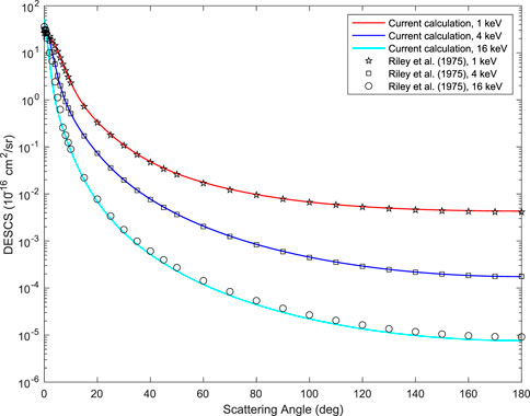
FIGURE 5. Differential elastic scattering cross-section of Al (solid line) as a function of the scattering angle (electron beam kinetic energy: 1 keV, 4 keV, 16 keV) compared to the Riley et al. calculations (Riley et al., 1975) (symbols).

2.2.6 Total elastic scattering cross-section and elastic mean free path

The total elastic scattering cross-section is given by

$\begin{array}{ll}\hfill {\sigma }_{\text{el}}& =\int \frac{d{\sigma }_{\text{el}}}{d\mathrm{\Omega }}d\mathrm{\Omega }\hfill \\ \hfill & ={\int }_0^{2\pi }d\phi {\int }_0^{\pi }d\vartheta \sin \vartheta \frac{d{\sigma }_{\text{el}}}{d\mathrm{\Omega }}\hfill \\ \hfill & =2\pi {\int }_0^{\pi }\frac{d{\sigma }_{\text{el}}}{d\mathrm{\Omega }}\sin \vartheta d\vartheta .\hfill \end{array}(66)$

Indicating with N the number of atoms per unit volume, the elastic mean free path is obtained by

${\lambda }_{\text{el}}=\frac{1}{N{\sigma }_{\text{el}}}.(67)$

2.2.7 Elastic cumulative probability

The cumulative probability P_el for elastic scattering collisions is another very important ingredient of the transport Monte Carlo method. It is given by

$P_{\text{el}}\left(\theta \right)=\frac{{\int }_0^{\theta }\frac{d{\sigma }_{\text{el}}}{d\mathrm{\Omega }}\sin \vartheta d\vartheta }{{\int }_0^{\pi }\frac{d{\sigma }_{\text{el}}}{d\mathrm{\Omega }}\sin \vartheta d\vartheta }=\frac{2\pi }{{\sigma }_{\text{el}}}{\int }_0^{\theta }\frac{d{\sigma }_{\text{el}}}{d\mathrm{\Omega }}\sin \vartheta d\vartheta .(68)$

2.3 Monte Carlo simulation

Monte Carlo modeling is very well known and we refer, in particular, to the code described in Ref. (Dapor, 2020). Details about the way in which we deal with the surface effects are described below. As usual, the step length Δs was calculated as

$\mathrm{\Delta }s=-\lambda \ln \mu ,(69)$

where μ is a random number uniformly distributed in the range [0,1] and λ = λ(E) is the electron mean free path, given by

$\lambda ={\left[{\lambda }_{\text{el}}^{-1}+{\lambda }_{\text{inel}}^{-1}\right]}^{-1}.(70)$

In this equation ${\lambda }_{\text{inel}}^{-1}$ is calculated using the bulk ELF, given by Eq. 35, if the electron is in the bulk. If, on the other hand, the electron is in the surface layer, ${\lambda }_{\text{inel}}^{-1}$ is calculated using the surface ELF, given by Eq. 50.

Ding et al. (2002) clarified that the surface scattering zone t_s extends into the solid and in the vacuum. Werner (2006) observed that the decay length of the surface excitations is of the order of t_s = v/ω_s, where v is the electron velocity. According to (Vicanek, 1999), we assume here that the thickness where surface plasmons are excited is given by v/2ω_s into the solid and v/2ω_s in the vacuum. Please note that, in the vacuum, ${\lambda }_{\text{el}}^{-1}=0$, so that if − v/2ω_s ≤ z ≤ 0 (z axis oriented from the surface toward the bulk), we have

$\lambda ={\lambda }_{\text{inel}},(71)$

where λ_inel is calculated using the surface ELF, given by Eq. 50. A similar approach is adopted for the calculation of the cumulative probabilities. If − v/2ω_s ≤ z ≤ v/2ω_s, then the inelastic cumulative probability is calculated using the surface ELF, given by Eq. 50. If z ≥ v/2ω_s, then the inelastic cumulative probability is calculated using the bulk ELF, given by Eq. 35. The cumulative probability of elastic scattering is calculated only when electrons are in the bulk.

The probability p_inel that the next collision be inelastic (surface or bulk, depending on z) is given by

$p_{\text{inel}}=\lambda {\lambda }_{\text{inel}}^{-1}.(72)$

Please note that, as a consequence, if − v/2ω_s ≤ z ≤ 0 then p_inel = 1.

Before each collision, if z ≥ 0, a random number uniformly distributed in the range [0,1] is generated and compared with the probability of inelastic scattering p_inel (surface or bulk, depending on z). If the random number is less than or equal to the probability of inelastic scattering, then the collision will be inelastic; otherwise, it will be elastic. On the other hand, if − v/2ω_s ≤ z ≤ 0, only surface plasmon excitations occur (no elastic collisions in this case).

In the case of inelastic collision, once the inelastic cumulative probability has been selected (surface or bulk), a random number uniformly distributed in the range [0,1] is generated and compared to the inelastic cumulative probability (as a function of the energy loss) in order to establish the energy loss. In the case of elastic collision, a random number uniformly distributed in the range [0,1] is generated and compared to the elastic cumulative probability (as a function of the scattering angle) in order to establish the scattering angle.

The azimuthal angle is calculated as a random number uniformly distributed in the range [0,2π].

The particles are followed in their trajectories until they leave the solid target or until their energy becomes lower than E₀-100 eV, where E₀ is the kinetic energy of the incident electron beam.

The present Monte Carlo program, written for simulating electron spectra and yields, is a user-friendly code freely obtainable on request to the author.

3 Results and discussion

Simulated spectra obtained according to our Monte Carlo model are presented in Figure 6 for electron initial kinetic energies 1,000, 2,000, 3,000, 5,000, and 10,000 eV. The number of simulated Monte Carlo trajectories for each spectrum was 10⁸. Monte Carlo simulation used the following conditions: 1) the angle between the sample surface normal and the incident electron beam’s direction was 0° (normal incidence), 2) the entrance aperture of the analyzer was from 0° to 90°, 3) the number of atoms per unit volume was N = 6.04 × 10²² atoms per cm³ (so the energy of the bulk plasmon peak derived from Eqs 20, 21 was 15.8 eV). All spectra were obtained by assuming a thickness t_s = v/ω_s for the region where surface plasmons are excited (−v/2ω_s ≤ z ≤ v/2ω_s). Over an energy loss region ranging from 0 to 100 eV, plasmon peaks up to the fifth order of scattering are clearly seen, while the sixth order of scattering plasmon peak is hardly observed. The mean energies of the higher-order peaks are multiple of the mean energy of the first-order plasmon peak for both bulk and surface inelastic scattering.

FIGURE 6

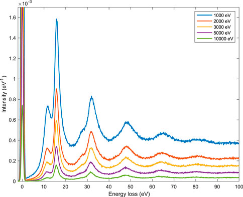
FIGURE 6. Simulated REEL spectra for 1,000–10,000 eV primary electrons. The number of simulated Monte Carlo trajectories was 10⁸. Monte Carlo simulation used the following conditions: (i) the angle between the sample surface normal and the incident electron beam’s direction was 0° (normal incidence), (ii) the entrance aperture of the analyzer was from 0° to 90°, (iii) the number of atoms per unit volume was N =6.04×10²² atoms per cm³ (so the energy of the bulk plasmon peak was 15.8 eV).

As for the first-order scattering, as expected the mean energy of the bulk plasmon peak is 15.8 eV. The surface plasmon peak is well resolved and its mean energy turns out to be ≈11.2 eV (in agreement with the theoretical prediction $\approx 15.8/\sqrt{2}$ eV = 11.2 eV). The ratio between the intensities of the surface and the bulk plasmon peaks decreases as the primary energy increases.

Please note that the simulated spectra were obtained assuming that the bulk plasmons’ relaxation time was twice the surface plasmons’ relaxation time. In this way, a reasonably good agreement was found between simulated and experimental data (see below).

The comparison between Monte Carlo and experimental data is shown in Figure 7 for the case of 1,000 eV initial kinetic energy and in Figure 8 for the case of 2,000 eV initial kinetic energy. The number of simulated Monte Carlo trajectories for these two simulations was 10⁹. For these two comparisons, Monte Carlo simulations used the experimental conditions, i.e., 1) the angle between the sample surface normal and the incident electron beam’s direction was 30°, 2) the entrance aperture of the analyzer was from 36° to 48°, 3) the number of atoms per unit volume was N = 5.47 × 10²² atoms per cm³. Please note that this lower density of the sample used for the measurement (as compared to the bulk and crystalline Al which is N = 6.04 × 10²² atoms per cm³) was experimentally determined. The lower density was ascribed to sputter-induced amorphization in the surface region. The energy of the bulk plasmon peak was, as a consequence, 15.0 eV instead of 15.8 eV. The lower density affects not only the mean energy of the plasmons but also the Fermi energy, the inelastic mean free path, and the elastic mean free path, which were, as a consequence, calculated according to this density before performing the Monte Carlo simulations presented in Figures 7, 8. Please note that, despite the proposed method’s simplicity, we found quite a good agreement between simulation and experiment, in particular for the first order of scattering plasmon peaks, presented in Figures 9, 10 for 1,000 eV and 2,000 eV electrons, respectively. The comparisons presented here show a better agreement with respect to similar approaches applied in the past (see, for example, Refs. (Calliari et al., 2007; Dapor et al., 2008; Dapor et al., 2011; Dapor et al., 2012)). It was obtained by the inclusion of the contribution of the inner shell electrons in the calculation of the dielectric function and to the consequent better description of the inelastic mean free path and of the inelastic cumulative probability for energies higher than 1,000 eV.

FIGURE 7

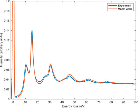
FIGURE 7. Experimental (blue line) and simulated (red line) REEL spectra for 1,000 eV primary electrons. The number of simulated Monte Carlo trajectories was 10⁹. Monte Carlo simulation used the experimental conditions: (i) the angle between the sample surface normal and the incident electron beam’s direction was 30°, (ii) the entrance aperture of the analyzer was from 36° to 48°, (iii) the number of atoms per unit volume was N =5.47×10²² atoms per cm³. Experimental data: Courtesy of Lucia Calliari and Massimiliano Filippi. The spectra were normalized to a common area of the zero-loss peak.

FIGURE 8

FIGURE 8. Experimental (blue line) and simulated (red line) REEL spectra for 2,000 eV primary electrons. The number of simulated Monte Carlo trajectories was 10⁹. Monte Carlo simulation used the experimental conditions: (i) the angle between the sample surface normal and the incident electron beam’s direction was 30°, (ii) the entrance aperture of the analyzer was from 36° to 48°, (iii) the number of atoms per unit volume was N =5.47×10²² atoms per cm³. Experimental data: Courtesy of Lucia Calliari and Massimiliano Filippi. The spectra were normalized to a common area of the zero-loss peak.

FIGURE 9

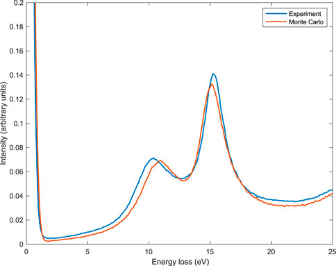
FIGURE 9. Experimental (blue line) and simulated (red line) REEL spectra for 1,000 eV primary electrons. The number of simulated Monte Carlo trajectories was 10⁹. Monte Carlo simulation used the experimental conditions: (i) the angle between the sample surface normal and the incident electron beam’s direction was 30°, (ii) the entrance aperture of the analyzer was from 36° to 48°, (iii) the number of atoms per unit volume was N =5.47×10²² atoms per cm³. Experimental data: Courtesy of Lucia Calliari and Massimiliano Filippi. The spectra were normalized to a common area of the zero-loss peak.

FIGURE 10

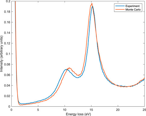
FIGURE 10. Experimental (blue line) and simulated (red line) REEL spectra for 2,000 eV primary electrons. The number of simulated Monte Carlo trajectories was 10⁹. Monte Carlo simulation used the experimental conditions: (i) the angle between the sample surface normal and the incident electron beam’s direction was 30°, (ii) the entrance aperture of the analyzer was from 36° to 48°, (iii) the number of atoms per unit volume was N =5.47×10²² atoms per cm³. Experimental data: Courtesy of Lucia Calliari and Massimiliano Filippi. The spectra were normalized to a common area of the zero-loss peak.

4 Conclusion

We simulated the reflection electron energy loss spectra for electron initial kinetic energies 1,000, 2,000, 3,000, 5,000, and 10,000 eV over an energy loss region ranging from 0 to 100 eV in order to investigate surface and bulk plasmon losses for incident electrons in Al. We observed plasmon peaks up to the fifth order of scattering and noted that, as expected, the ratio between the intensities of the surface and the bulk plasmon peaks decreases as the primary energy increases. We also compared experimental data to Monte Carlo simulations concerning reflection electron energy loss spectra. We found reasonable agreement between experimental and simulated data for 1,000 eV and 2000 eV assuming that the relaxation time of the bulk plasmons was two times the relaxation time of the surface plasmons.

Data availability statement

The original contributions presented in the study are included in the article/supplementary material, further inquiries can be directed to the corresponding author.

Author contributions

MD: Conceptualization, Methodology, Writing—original draft, Project administration, Funding acquisition.

Acknowledgments

I wish to express my sincere gratitude to Pablo de Vera (Murcia University) and to Giovanni Garberoglio and Simone Taioli (European Centre for Theoretical Studies in Nuclear Physics and Related Areas (ECT*-FBK) in Trento) for their invaluable and stimulating comments. I am also grateful to Maria Del Huerto Flammia (Fondazione Bruno Kessler) for assisting me with the proofreading of this article.

Conflict of interest

The author declares that the research was conducted in the absence of any commercial or financial relationships that could be construed as a potential conflict of interest.

Publisher’s note

All claims expressed in this article are solely those of the authors and do not necessarily represent those of their affiliated organizations, or those of the publisher, the editors and the reviewers. Any product that may be evaluated in this article, or claim that may be made by its manufacturer, is not guaranteed or endorsed by the publisher.

Footnotes

¹Please note that if, in the Drude-Lorenz theory, the field is described by the equation

$\mathbf{E}={\mathbf{E}}_0\exp \left(-i\omega t\right)(23)$

instead of Eq. 2, the following equation

$\mathbf{r}={\mathbf{r}}_0\exp \left(-i\omega t\right),(24)$

has to be used instead of Eq. 3. Then, for the case of free oscillators, for example, the dielectric function assumes the following form

$\epsilon \left(\omega \right)=1-\frac{{\omega }_p^2}{{\omega }^2+i\omega {\gamma }_0},(25)$

Using Eq. 14, ɛ₂(ω) is negative [see Eq. 17], while, using Eq. 25, ɛ₂(ω) is given by

${\epsilon }_2\left(\omega \right)=\frac{{\gamma }_0}{\omega }\frac{{\omega }_p^2}{{\omega }^2+{\gamma }_0^2},(26)$

and is positive. To make the ELF positive using Eq. 25, the energy loss function is defined as the imaginary part of the opposite of the dielectric function:

$f\left(\omega \right)=\mathrm{I}\mathrm{m}\left[-\frac{1}{\epsilon \left(\omega \right)}\right]=\frac{{ϵ}_2\left(\omega \right)}{{ϵ}_1^2\left(\omega \right)+{ϵ}_2^2\left(\omega \right)}.(27)$

So it is clear that the sign is just a matter of the choice of the function describing the time dependence of the electron displacement. In this paper, we will use Eq. 3 and the definition given by Eq. 28, so the ELF is defined as the imaginary part of the reciprocal of the dielectric function, since ɛ₂(ω) is negative.

²Please note that a further improvement of the description of the REEL spectra could be obtained taking into account that also the dispersion law is affected by surface effects. Due to a quasi-2D slab on the top of bulk, a more general dispersion law was proposed by Kyriakou et al. (2011), i.e.,

${\hslash }^2{\omega }_k^2=\hslash {\omega }_p\sqrt{\frac{6E_{\mathrm{F}}}{5}\frac{{\hslash }^2{k}^2}{2m}}+\frac{12E_{\mathrm{F}}}{5}\frac{{\hslash }^2{k}^2}{2m}+{\left(\frac{{\hslash }^2{k}^2}{2m}\right)}^2.(51)$

For the calculations presented in this paper, we did not use this dispersion law. Its inclusion in the calculations will be the subject of future investigations.

References

Abril, I., Garcia-Molina, R., Denton, C. D., Pérez-Pérez, F. J., and Arista, N. R. (1998). Dielectric description of wakes and stopping powers in solids. Phys. Rev. A . Coll. Park. 58, 357–366. doi:10.1103/physreva.58.357

CrossRef Full Text | Google Scholar

Ashcroft, N. W., and Mermin, N. D. (1976). Solid state physics. Belmont: Harcourt College Publishers.

Google Scholar

Ashley, J. C. (1990). Energy loss rate and inelastic mean free path of low-energy electrons and positrons in condensed matter. J. Electron Spectrosc. Relat. Phenom. 50, 323–334. doi:10.1016/0368-2048(90)87075-y

CrossRef Full Text | Google Scholar

Bourke, J. D., and Chantler, C. T. (2012). Electron energy loss spectra and overestimation of inelastic mean free paths in many-Pole models. J. Phys. Chem. A 116, 3202–3205. doi:10.1021/jp210097v

PubMed Abstract | CrossRef Full Text | Google Scholar

Bunyan, P. J., and Schonfelder, J. L. (1965). Polarization by mercury of 100 to 2000 eV electrons. Proc. Phys. Soc. 85, 455–462. doi:10.1088/0370-1328/85/3/306

CrossRef Full Text | Google Scholar

Burke, P. G., and Joachain, C. J. (1995). Theory of electron-atom collisions. New York: Plenum Press.

Google Scholar

Calliari, L., Dapor, M., and Filippi, M. (2007). Joint experimental and computational study of aluminum electron energy loss spectra. Surf. Sci. 601, 2270–2276. doi:10.1016/j.susc.2007.03.029

CrossRef Full Text | Google Scholar

Chen, Y. F., and Kwei, C. M. (1996). Electron differential inverse mean free path for surface electron spectroscopy. Surf. Sci. 364, 131–140. doi:10.1016/0039-6028(96)00616-4

CrossRef Full Text | Google Scholar

Chiarello, G., Colavita, E., De Crescenzi, M., and Nannarone, S. (1984). Reflection electron-energy-loss investigation of the electronic and structural properties of palladium. Phys. Rev. B 29, 4878–4889. doi:10.1103/physrevb.29.4878

CrossRef Full Text | Google Scholar

Cox, H. L., and Bonham, R. A. (1967). Elastic electron scattering amplitudes for neutral atoms calculated using the partial wave method at 10, 40, 70, and 100 kV for Z = 1 to Z = 54. J. Chem. Phys. 47, 2599–2608. doi:10.1063/1.1712276

CrossRef Full Text | Google Scholar

Dapor, M., Calliari, L., and Filippi, M. (2008). REEL spectra from aluminium: experiment and Monte Carlo simulation using two different dielectric functions. Surf. Interface Anal. 40, 683–687. doi:10.1002/sia.2711

CrossRef Full Text | Google Scholar

Dapor, M., Calliari, L., and Scarduelli, G. (2011). Comparison between Monte Carlo and experimental aluminum and silicon electron energy loss spectra. Nucl. Instrum. Methods Phys. Res. Sect. B Beam Interact. Mater. Atoms 269, 1675–1678. doi:10.1016/j.nimb.2010.11.030

CrossRef Full Text | Google Scholar

Dapor, M., Calliari, L., and Fanchenko, S. (2012). Energy loss of electrons backscattered from solids: Measured and calculated spectra for Al and Si. Surf. Interface Anal. 44, 1110–1113. doi:10.1002/sia.4835

CrossRef Full Text | Google Scholar

Dapor, M. (1995a). Elastic scattering of electrons and positrons by atoms. Differential and transport cross section calculations. Nucl. Instrum. Methods Phys. Res. Sect. B Beam Interact. Mater. Atoms 95, 470–476. doi:10.1016/0168-583x(95)00003-8

CrossRef Full Text | Google Scholar

Dapor, M. (1995b). Analytical transport cross section of medium energy positrons elastically scattered by complex atoms (Z=1–92). J. Appl. Phys. 77, 2840–2842. doi:10.1063/1.358697

CrossRef Full Text | Google Scholar

Dapor, M. (1996). Elastic scattering calculations for electrons and positrons in solid targets. J. Appl. Phys. 79, 8406–8411. doi:10.1063/1.362514

CrossRef Full Text | Google Scholar

Dapor, M. (2003). Electron-beam interaction with solids: Applications of the Monte Carlo method to electron scattering problems. Berlin: Springer.

Google Scholar

Dapor, M. (2015). Mermin differential inverse inelastic mean free path of electrons in polymethylmethacrylate. Front. Mater. 2, 1–3. doi:10.3389/fmats.2015.00027

CrossRef Full Text | Google Scholar

Dapor, M. (2017). Role of the tail of high-energy secondary electrons in the Monte Carlo evaluation of the fraction of electrons backscattered from polymethylmethacrylate. Appl. Surf. Sci. 391, 3–11. doi:10.1016/j.apsusc.2015.12.043

CrossRef Full Text | Google Scholar

Dapor, M. (2020). “Transport of energetic electrons in solids,” in Springer tracts in modern Physics (Springer Nature Switzerland AG), 271.

Google Scholar

Dapor, M. (2022a). Electron-atom collisions. Quantum-relativistic theory and exercises. Berlin: De Gruyter.

Google Scholar

Dapor, M. (2022b). Differential elastic scattering cross-section of spin-polarized electron beams impinging on uranium. J. Phys. B At. Mol. Opt. Phys. 55, 0952021–0952029. doi:10.1088/1361-6455/ac61ee

CrossRef Full Text | Google Scholar

de Vera, P., and Garcia-Molina, R. (2019). Electron inelastic mean free paths in condensed matter down to a few electronvolts. J. Phys. Chem. C 123, 2075–2083. doi:10.1021/acs.jpcc.8b10832

CrossRef Full Text | Google Scholar

Denton, C. D., Abril, I., Garcia-Molina, R., Moreno-Marin, J. C., and Heredia-Avalos, S. (2008). Influence of the description of the target energy-loss function on the energy loss of swift projectiles. Surf. Interface Anal. 40, 1481–1487. doi:10.1002/sia.2936

CrossRef Full Text | Google Scholar

Ding, Z. J., Li, H. M., Pu, Q. R., Zhang, Z. M., and Shimizu, R. (2002). Reflection electron energy loss spectrum of surface plasmon excitation of Ag: A Monte Carlo study. Phys. Rev. B 66, 085411–085417. doi:10.1103/physrevb.66.085411

CrossRef Full Text | Google Scholar

Egerton, R. F. (2011). Electron energy-loss spectroscopy in the electron microscope. Third Edition. Berlin: Springer.

Google Scholar

Furness, J. B., and McCarthy, I. E. (1973). Semiphenomenological optical model for electron scattering on atoms. J. Phys. B At. Mol. Phys. 6, 2280–3229 1. doi:10.1088/0022-3700/6/11/021

CrossRef Full Text | Google Scholar

Henke, B. L., Gullikson, E. M., and Davis, J. C. (1993). X-ray interactions: Photoabsorption, scattering, transmission, and reflection at E = 50 − 30, 000 eV, Z = 1 − 92. Atomic Data Nucl. Data Tables 54, 181–342. doi:10.1006/adnd.1993.1013

CrossRef Full Text | Google Scholar

Jablonski, A., and Powell, C. J. (2004). Information depth for elastic-peak electron spectroscopy. Surf. Sci. 551, 106–124. doi:10.1016/j.susc.2003.12.036

CrossRef Full Text | Google Scholar

Jablonski, A., Salvat, F., and Powell, C. J. (2004). Comparison of electron elastic-scattering cross sections calculated from two commonly used atomic potentials. J. Phys. Chem. Reference Data 33, 409–451. doi:10.1063/1.1595653

CrossRef Full Text | Google Scholar

Jablonski, A. (1991). Elastic electron backscattering from gold. Phys. Rev. B 43, 7546–7554. doi:10.1103/physrevb.43.7546

PubMed Abstract | CrossRef Full Text | Google Scholar

Joy, D. C. (1995). Monte Carlo modeling for electron microscopy and microanalysis. Oxford: Oxford University Press.

Google Scholar

Kessler, J. (1985). Polarized electrons. Berlin: Springer.

Google Scholar

Kyriakou, I., Emfietzoglou, D., Garcia-Molina, R., Abril, I., and Kostarelos, K. (2011). Simple model of bulk and surface excitation effects to inelastic scattering in low-energy electron beam irradiation of multi-walled carbon nanotubes. J. Appl. Phys. 110, 0543041–543112. doi:10.1063/1.3626460

CrossRef Full Text | Google Scholar

Lin, S.-R., Sherman, N., and Percus, J. K. (1963). Elastic scattering of relativistic electrons by screened atomic nuclei. Nucl. Phys. 45, 492–504. doi:10.1016/0029-5582(63)90824-1

CrossRef Full Text | Google Scholar

Mayol, R., and Salvat, M. (1997). Total and transport cross sections for elastic scattering of electrons by atoms. At. Data Nucl. Data Tables 65, 55–154. doi:10.1006/adnd.1997.0734

CrossRef Full Text | Google Scholar

Mermin, N. D. (1970). Lindhard dielectric function in the relaxation-time approximation. Phys. Rev. B 1, 2362–2363. doi:10.1103/physrevb.1.2362

CrossRef Full Text | Google Scholar

Mott, N. F. (1929). The scattering of fast electrons by atomic nuclei. Proc. R. Soc. Lond. 124, 425–442.

Google Scholar

Ohno, Y. (1989). Kramers-krönig analysis of reflection electron-energy-loss spectra measured with a cylindrical mirror analyzer. Phys. Rev. B 39, 8209–8219. doi:10.1103/physrevb.39.8209

PubMed Abstract | CrossRef Full Text | Google Scholar

Penn, D. R. (1987). Electron mean-free-path calculations using a model dielectric function. Phys. Rev. B 35, 482–486. doi:10.1103/physrevb.35.482

PubMed Abstract | CrossRef Full Text | Google Scholar

Riley, M. E., MacCallum, J., and Biggs, F. (1975). Theoretical electron-atom elastic scattering cross sections. Selected elements, 1 keV to 256 keV. At. Data Nucl. Data Tables 15, 443–476. doi:10.1016/0092-640X(75)90012-1

CrossRef Full Text | Google Scholar

Ritchie, R. H., and Howie, A. (1977). Electron excitation and the optical potential in electron microscopy. Philos. Mag. 36, 463–481. doi:10.1080/14786437708244948

CrossRef Full Text | Google Scholar

Ritchie, R. H. (1957). Plasma losses by fast electrons in thin films. Phys. Rev. 106, 874–881. doi:10.1103/physrev.106.874

CrossRef Full Text | Google Scholar

Salvat, F., and Mayol, R. (1993). Elastic scattering of electrons and positrons by atoms. Schrödinger and Dirac partial wave analysis. Comput. Phys. Commun. 74, 358–374. doi:10.1016/0010-4655(93)90019-9

CrossRef Full Text | Google Scholar

Salvat, F., Martinez, J. D., Mayol, R., and Parellada, J. (1987). Analytical Dirac-Hartree-Fock-slater screening function for atoms (Z=1-92). Phys. Rev. A . Coll. Park. 36, 467–474. doi:10.1103/physreva.36.467

PubMed Abstract | CrossRef Full Text | Google Scholar

Salvat, F., Jablonski, A., and Powell, C. J. (2005). ELSEPA - Dirac partial-wave calculation of elastic scattering of electrons and positrons by atoms, positive ions and molecules. Comput. Phys. Commun. 165, 157–190. doi:10.1016/j.cpc.2004.09.006

CrossRef Full Text | Google Scholar

Salvat, F. (2003). Optical-model potential for electron and positron elastic scattering by atoms. Phys. Rev. A . Coll. Park. 68, 0127081–127117. doi:10.1103/physreva.68.012708

CrossRef Full Text | Google Scholar

Shimizu, R., and Ding, Z. J. (1992). Monte Carlo modelling of electron-solid interactions. Rep. Prog. Phys. 55, 487–531. doi:10.1088/0034-4885/55/4/002

CrossRef Full Text | Google Scholar

Tanuma, S., Powell, C. J., and Penn, D. R. (1988). Calculations of electron inelastic mean free paths for 31 materials. Surf. Interface Anal. 11, 577–589. doi:10.1002/sia.740111107

CrossRef Full Text | Google Scholar

Tanuma, S., Powell, C. J., and Penn, D. R. (2004). Calculations of electron inelastic mean free paths. VIII. Data for 15 elemental solids over the 50-2000 eV range. Surf. Interface Anal. 36, 1–14. doi:10.1002/sia.1997

CrossRef Full Text | Google Scholar

Tung, C. J., Chen, Y. F., Kwei, C. M., and Chou, T. L. (1994). Differential cross sections for plasmon excitations and reflected electron-energy-loss spectra. Phys. Rev. B 49, 16684–16693. doi:10.1103/physrevb.49.16684

PubMed Abstract | CrossRef Full Text | Google Scholar

Vicanek, M. (1999). Electron transport processes in reflection electron energy loss spectroscopy (REELS) and X-ray photoelectron spectroscopy (XPS). Surf. Sci. 440, 1–40. doi:10.1016/s0039-6028(99)00784-0

CrossRef Full Text | Google Scholar

Werner, W. S. M., Smekal, W., Tomastik, C., and Stoöri, H. (2001). Surface excitation probability of medium energy electrons in metals and semiconductors. Surf. Sci. 486, L461–L466. doi:10.1016/s0039-6028(01)01091-3

CrossRef Full Text | Google Scholar

Werner, W. S. M. (2006). Differential surface and volume excitation probability of medium-energy electrons in solids. Phys. Rev. B 74, 075421–75514. doi:10.1103/physrevb.74.075421

CrossRef Full Text | Google Scholar

Yubero, F., and Tougaard, S. (1992). Model for quantitative analysis of reflection-electron-energy-loss spectra. Phys. Rev. B 46, 2486–2497. doi:10.1103/physrevb.46.2486

PubMed Abstract | CrossRef Full Text | Google Scholar

Yubero, F., Sanz, J. M., Elizalde, E., and Galán, L. (1990). Kramers-krönig analysis of reflection electron energy loss spectra (REELS) of Zr and ZrO₂. Surf. Sci. 237, 173–180. doi:10.1016/0039-6028(90)90529-h

CrossRef Full Text | Google Scholar