- 1Fraunhofer Institute for Mechanics of Materials IWM, Freiburg, Germany
- 2Intelligent Systems Research Group ISRG, Karlsruhe University of Applied Sciences, Karlsruhe, Germany
- 3Institute for Applied Materials—Computational Materials Sciences IAM-CMS, Karlsruhe Institute of Technology, Karlsruhe, Germany
In materials design, supervised learning plays an important role for optimization and inverse modeling of microstructure-property relations. To successfully apply supervised learning models, it is essential to train them on suitable data. Here, suitable means that the data covers the microstructure and property space sufficiently and, especially for optimization and inverse modeling, that the property space is explored broadly. For virtual materials design, typically data is generated by numerical simulations, which implies that data pairs can be sampled on demand at arbitrary locations in microstructure space. However, exploring the space of properties remains challenging. To tackle this problem, interactive learning techniques known as active learning can be applied. The present work is the first that investigates the applicability of the active learning strategy query-by-committee for an efficient property space exploration. Furthermore, an extension to active learning strategies is described, which prevents from exploring regions with properties out of scope (i.e., properties that are physically not meaningful or not reachable by manufacturing processes).
1 Introduction
1.1 Motivation
With regard to natural learning processes, Cohn et al. stated that “in many situations, the learner’s most powerful tool is its ability to act, to gather data, and to influence the world it is trying to understand” (Cohn et al., 1996). One attempt to transfer this ability to methods in the field of machine learning is called active learning. Active learning describes an interactive learning process in which machine learning models improve with experience and training (Settles, 2012). It is therefore contrary to the often used approach of gathering data a priori and learn from it afterwards. In fact, active learning couples both, sampling and training, what typically results in an efficient and broad data space exploration.
In terms of materials design, the exploration of data spaces is quite important. For a designer, it is essential to know all possible microstructure configurations and reachable properties of a material in order to increase the performance of a workpiece. How to delineate these configurations and properties is described for example in the microstructure sensitive design (MSD) approach (Adams et al., 2001). Two necessary steps for MSD are 1) to determine the design space yielding a hull of possible microstructures and 2) to calculate the corresponding properties defining a so-called property closure (Fullwood et al., 2010). For complex high-dimensional microstructure representations, exploring the design space is, however, challenging. It is even more challenging, if gathering data is cumbersome, because it is time-consuming (e.g., running complex numerical simulations), ties up manpower (e.g., labeling data manually) or laborious (e.g., performing experiments).
To the authors knowledge, the present work is the first one that uses the active learning strategy query-by-committee (Burbidge et al., 2007) for generating microstructure-property data in materials science. We show that the active learning strategy can be used to explore microstructure-property spaces efficiently and that the generated data is better suited to train accurate machine learning models than data generated via classical sampling approaches. Moreover, we present an extension to active learning approaches that aims to avoid sampling in regions with properties out of scope. This is necessary, as defining bounds for microstructure spaces is not always simple and it can happen that active learning techniques explore regions with properties that are physically not meaningful or not reachable by manufacturing processes.
1.2 Related Work
Active learning techniques can be grouped into three use-case specific classes, namely stream-based selective sampling, pool-based selective sampling and membership query synthesis (Settles, 2009). The first two mentioned are based either on a continuous data-stream or an a priori defined pool of data, from which the active learning algorithm can chose data points to be labeled. In membership query synthesis, in contrast, the algorithm is free of choice at which location new data points are created. Therefore, membership query synthesis is well suited for virtual data generation on the basis of numerical simulations.
Membership query synthesis goes back to Angluin (1988) for classification problems and to Cohn et al. (1996) for regression problems. The technique presented in Cohn et al. (1996) is called variance reduction. It aims to minimize the output variance of a machine learning model in order to minimize the future generalization error. Alternative approaches for regression problems are maximizing the expected change of a machine learning model when seeing new data (Cai et al., 2013) or committee-based approaches like query-by-committee (Burbidge et al., 2007), where the prediction variance of a committee consisting of multiple separately trained machine learning models is minimized. In the present study, we use the latter approach, as it is straightforward to implement and scales to complex models (i.e., neural networks). Recent research in active learning targets the application of deep learning models, see for example Stark et al. (2015) and Wang et al. (2016) for applications using convolutional neural networks and Zhu and Bento (2017), Sinha et al. (2019) and Mayer and Timofte (2020) for generative models.
Instead of actively sampling data spaces, classical space-filling sampling strategies can be used to generate data without considering the learning task, see Fang et al. (2000), Simpson et al. (2001) and Wang and Shan (2006) for an overview. In the following, we list some of the most popular space-filling sampling strategies. Latin hypercube design (McKay et al., 2000) aims to partition the dimensions of the input space into equidistant slices and places data points such that each slice is covered by one data point. Orthogonal arrays (Owen, 1992) are special matrices that define sampling with the aim to sample data spaces uniformly. In particular, orthogonal arrays can be used to generate uniform Latin hypercubes (Tang, 1993). Furthermore, low-discrepancy sequences can be used to cover spaces uniformly with data points, see for example Niederreiter (1988). Among others, popular sequences are the Hammersley sequence (Hammersley and Handscomb, 1964), Halton sequence (Halton, 1964) and Sobol sequence (Sobol, 1967). In addition to these methods, a common sampling strategy is to randomly draw samples from a uniform distribution. However, all of these approaches suffer from the curse of dimensionality, which means that the effort needed to sufficiently sample data spaces grows exponentially with the number of dimensions.
In materials design, the usage of classical sampling strategies is very common. The framework for data-driven analysis of materials that is presented in Bessa et al. (2017) for example, uses data generation on the basis of space-filling sampling methods, especially the Sobol sequence. In Gupta et al. (2015), dual-phase 2D-microstructures are generated by randomly placing particles in a steel matrix. In order to generate spatially resolved dual-phase microstructure volume elements, Liu et al. (2015b) uses evenly distributed data of phase volume fractions. Regarding homogenized microstructural features, in Iraki et al. (2021), Latin hypercube design is used to generate a data set of textures for cold rolled steel sheets. Even special sampling heuristics have been developed for generating sets of microstructure features, like in Johnson and Kurniawan, 2018.
Also, adaptive sampling techniques are used in materials design, however, in the sense of an optimization aiming to identify microstructures with targeted properties. In Liu et al. (2015a) and Paul et al. (2019), specific machine learning-based optimization approaches are presented that efficiently guide sampling to regions in the space of microstructures, where microstructures with desired properties are expected to be located. Further statistic-based approaches exist that use surrogate-based optimization (cf. Forrester and Keane, 2009), see Nikolaev et al. (2016), Balachandran et al. (2016), Lookman et al. (2017) and Lookman et al. (2019). Yet, as these approaches aim to find individual material compositions or microstructures for certain target properties, they are not applicable for sampling microstructure-property spaces broadly.
So far, only few publications exist, which describe the usage of active learning to train a machine learning model while generating microstructure-property data (Jung et al., 2019; Kalidindi, 2019; Castillo et al., 2019). The approaches presented therein are based on variance reduction using Bayesian models, like Gaussian process regression (GPR), cf. Seo et al. (2000). Such Bayesian approaches can have a tremendous advantage when working with experimental measurements. However, the computational complexity of GPR increases cubically with the number of data points. Furthermore, it is worth mentioning the Bayesian approach described in Tran and Wildey (2021) to solve stochastic inverse problems for property-structure linkages. It is the aim of the approach to model posterior probabilities for microstructures having desired properties. This is achieved by successively updating an a priori probability distribution with new sampled microstructure-property data points. These are generated by drawing microstructure samples from the actual probability distribution and evaluating their properties. Afterwards, the samples are accepted or rejected depending on a certain criterion. However, this so-called acceptance-rejection sampling can be disadvantageous in terms of sample efficiency, as the decision to accept samples is made after calculating properties.
1.3 Paper Structure
In Section 2 the concept of membership query synthesis is presented including an extension to avoid sampling in regions out of scope. Additionally, the applied query-by-committee approach is described in detail. In Section 3, three numerical examples are shown to demonstrate the advantage of using active learning to sample microstructure-property spaces. The results are discussed in Section 4. The work is summarized in Section 5 and a brief outlook on the application of active learning in virtual materials design is given.
2 Methods
2.1 Active Learning via Membership Query Synthesis
Membership query synthesis follows an iterative procedure that is sketched schematically in Figure 1, cf. Settles (2012). The procedure starts with an initial data set of input variables
where
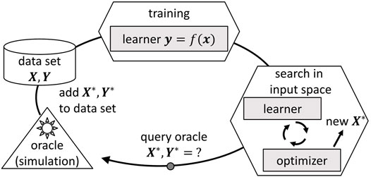
FIGURE 1. Iterative procedure of membership query synthesis, cf. Settles (2012).
2.2 Avoid Queries in Regions out of Scope
Following the procedure described in Section 2.1, new data points are generated over the whole input space. In many applications, this might be appropriate to improve the learner. However, when the input space bounds cannot be defined adequately, it is probable that the active learning algorithm queries for data in regions that are out of interest for the application case. To avoid sampling in regions out of scope, the original workflow depicted in Figure 1 can be extended with a region, cf. Figure 2. The purpose of the region filter is to limit the optimizer to regions in the input space leading only to output quantities of interest. In order to set up the region filter, the data points Xi get an additional class label c ∈ (0, 1), which marks if the output values are of interest or out of scope. The bounds in the output space that determine the class label can be defined by the user.
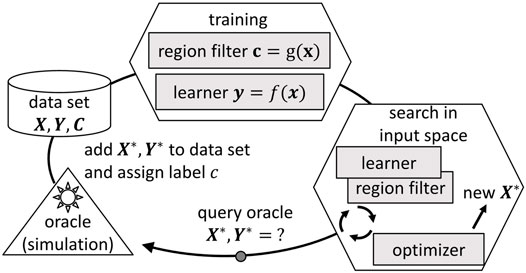
FIGURE 2. Iterative procedure of membership query synthesis (cf. Settles (2012)) including an extension to avoid sampling in regions out of scope. The class labels of the data points are represented by Ci ∈ (0, 1).
The region filter is realized by a binary classifier that partitions the input space depending on the class label by learning the mapping function
In fact, the described extension is similar to Bayesian optimization approaches that account for unknown constraints using classification methods, see for example Sacher et al. (2018), Heese et al. (2019) and Tran et al. (2019).
Often the amount of data that is out of scope is much lower than the data of interest. If this is the case, one-class classification methods can be used as region filter, such as isolation forests (Liu et al., 2008) or one-class support vector machines (Schölkopf et al., 2001). Both are unsupervised learning methods that delimit the input space, which is covered by data out of scope. Once trained, they are used to estimate the class membership of unseen data points. For more complex classification problems, this can also be achieved by deep learning approaches (cf. Chalapathy and Chawla, 2019), such as autoencoder neural networks (Hinton and Salakhutdinov, 2006; Sakurada and Yairi, 2014).
2.3 Query-By-Committee for Microstructure-Property Space Exploration
Originally, query-by-committee was introduced by Seung et al. (1992) for classification problems. In this study, the query-by-committee approach following Burbidge et al. (2007) for regression problems is applied. In this approach, the learner is realized by a committee of n regression models (here we use feedforward neural networks). Following the workflow depicted in Figure 1, the committee members are trained on the actual data set. However, in this work, each neural network is trained only on a subset of the data (RayChaudhuri and Hamey, 1995). In order to query new data points, the microstructure space is searched for the location at which the committee members disagree the most. Disagreement is defined by the variance of the neural network predictions s2 (Krogh and Vedelsby, 1995):
where fη (x) denotes the property prediction of neural network η and
Certainly, it is challenging here to chose the right number of regression models and to equip them with sufficient complexity (e.g., depth of neural networks). Depending on the mapping to learn, we suggest to assign a lower complexity to the regression models in the beginning, as the amount of initial data is typically low. With an increasing amount of data it is possible to increase the complexity of the regression models, which was, however, not done in this study. Regarding the number of regression models in the committee, the similarity of the query-by-committee approach to Bayesian methods like GPR is worth mentioning here. GPR can be interpreted as a distribution over functions (Williams and Rasmussen, 2006), which is also the case for the query-by-committee approach when the number of committee members goes to infinity. Though, the overall training time of the query-by-committee approach increases linearly with an increasing number of committee members.
In order to extend the query-by-committee approach to avoid sampling in regions out of scope, first, data points that exceed the predefined output bounds need to be filtered out from the actual data set. Then, a classifier is trained on these data points in order to delimit a region in microstructure space. This region is excluded from the optimization by adding a soft constraint to Eq. 4:
where ⟨⋅⟩ denotes the Macaulay brackets and ρ(x) denotes the distance of x to the decision boundary that is defined by the classifier. As s2(x) and ρ(x) can be of different magnitudes, the scalar weight factor W is introduced, which needs to be set in order to balance the optimization.
In this work, ρ(x) is determined by an isolation forest classifier. Isolation forest is an outlier detection method that consists of an ensemble of decision trees. Each tree partitions the input space randomly until all training data points are isolated. It is assumed that outliers typically lie in partitions with rather short paths in the decision tree structures. On the basis of the path lengths, an anomaly score (in the range of (0, 1)) can be defined for each observation, see Liu et al. (2008) for details. Therein, it is stated that data points with an anomaly score
To solve Eqs 4, 5, we use the differential evolution algorithm by Storn and Price (1997) as it is implemented in Python package scipy (Virtanen et al., 2020). The neural network models and the isolation forest classifier applied in this work are based on the implementation in Python package scikit-learn (Pedregosa et al., 2011).
3 Results
3.1 Toy Example: Dirac Delta Function
First, a simplistic extreme case is analyzed. The data generating process considered here is given by an approximation of the Dirac delta function via a Gaussian distribution
with parameter α = 0.1. A set of 500 data points is generated by randomly drawing samples of x in the range of (−50, 50). Additionally, 500 data points are generated via query-by-committee. Therefore, a committee of five neural networks is set up, which are all trained on a random subset of 80% of the actual data. The neural networks consist of two layers with five neurons each. To avoid overfitting, early stopping (Prechelt, 1998) and L2-regularization (Krogh and Hertz, 1992) is applied with regularization parameter λ = 0.0001. As activation functions, rectifiers (ReLU) are used. The mean-squared-error loss function between true and predicted δ(x) is applied and optimized using the limited-memory Broyden-Fletcher-Goldfarb-Shanno (BFGS) optimizer (Liu and Nocedal, 1989). The approach is initialized with 100 randomly drawn samples.
The resulting 500 data points and their distribution over x are shown in Figure 3. The data points generated by random sampling are distributed almost uniformly over the input space. All data points are located in regions of lower δ(x). The maximum δ(x)-value in the randomly sampled data set equals 0.506 208 09. In contrast, the query-by-committee approach concentrates on sampling the region close to the peak of the approximated delta function. The maximum δ(x)-value in the data set equals 5.64189535, which is very close to the maximum of Eq. 6: δ(x = 0) = 5.64189584. The generated data is available online, see Morand et al. (2021).
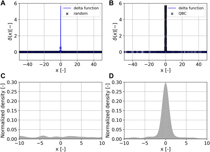
FIGURE 3. The sampled input-output space of the approximated Dirac delta function δ(x) is shown above. 500 samples were generated via random sampling (A) and query-by-committee, labeled as QBC, (B). Below, the normalized Gaussian kernel density estimation is shown for the data sets generated via random sampling (C) and query-by-committee (D).
3.2 Identifying Material Model Parameters
The second example is about inferring material model parameters from given material model responses, which is (like typical materials design problems) an inverse identification problem, cf. Mahnken (2004). To solve it, neural networks can be used to directly learn a mapping from material model responses to model parameters (Yagawa and Okuda, 1996; Huber, 2000). Such an approach is for example applied in Huber and Tsakmakis (1999) to identify constitutive parameters of a finite deformation plasticity model on the basis of spherical indentation tests. As simulating spherical indentation tests is time consuming, the usage of active learning can be beneficial, because it efficiently explores the space of material model parameters and responses. This characteristic can be understood as goal-directed sampling, which is essential for the prediction quality of supervised learning models that are directly trained on inverse relations (Jordan and Rumelhart, 1992).
In this example, we analyze the identification problem described in Morand and Helm (2019), as it requires a special sampling, for which a knowledge-based approach has been developed. The data generating process is defined by the hardening model (cf. Helm, 2006):
where β and γ are material dependent parameters and sp denotes the accumulated plastic strain. For the purpose of this study, the hardening curves are discretized into 20 equidistantly distributed points in sp ∈ (0.0, 0.2). For sampling, we consider β and
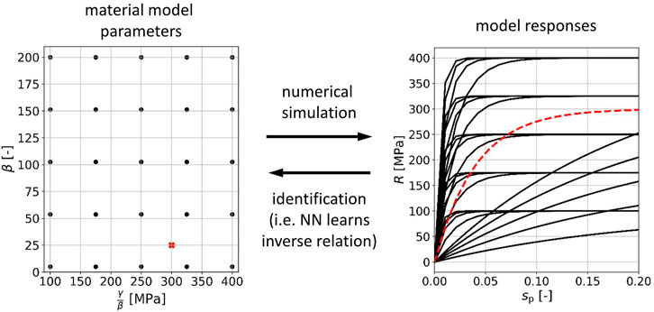
FIGURE 4. Parameter identification problem. A data base of material model parameters and corresponding responses is set up (black dots and curves), which can be used to train a neural network (NN) on the inverse mapping. After training, the neural network is able to identify parameters for given hardening curves (red dashed line and cross).
In total 2,500 discretized hardening curves
The resulting sets of parameter tuples (β,
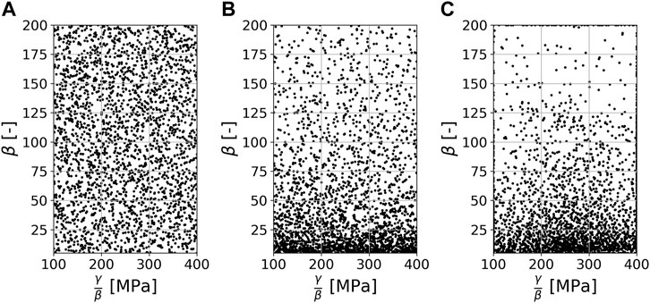
FIGURE 5. The sampled parameter space of the hardening model described in Eq. 7. 2,500 samples were generated using Latin hypercube design (A), the knowledge-based sampling approach following Morand and Helm (2019) (B) and query-by-committee (C).
In order to show these effects, neural networks are trained on the data sets. As there is no ground truth to test the trained models, the generated data is also used for testing. Training and testing is done for both, the forward mapping
and the inverse mapping as it is outlined in Figure 4
where
The neural networks that learn the forward mapping consist of two hidden layers with 10 and 15 neurons and for learning the inverse mapping they consist of two hidden layers with 15 and 10 neurons. In both cases, the mean-squared-error loss function between true and predicted output quantity is applied and optimized using the limited-memory BFGS optimizer with L2 regularization of λ = 0.0001. Furthermore, early stopping is applied using a random subset of 10% of the training data for validation. Both networks use ReLU activation functions. To measure the performance of the forward models, the absolute error between the predicted curve Hpred and the true curve Htrue is given by
To measure the performance of the inverse models, the curves are reconstructed using the predicted material model parameters (which yields Hrecon) and compared with the true curves Htrue:
Training and test runs were performed five times with different random validation splits. The averaged results are listed in Table 1. The neural network trained on the data set generated by query-by-committee reaches a similar performance than the neural network trained on the data generated by the knowledge-based approach when tested on the Latin hypercube samples. When tested on each other, the averaged mean is rather low for both approaches. However, one can observe that for modeling the forward relation, the neural network trained with the data generated by query-by-committee is slightly better than the one trained with the data generated by the knowledge-based sampling approach and vice versa for the inverse relation. Comparing both neural networks with the neural network trained on the data generated via Latin hypercube design, the latter is outperformed for every test set. The generated data is available online, see Morand et al. (2021).

TABLE 1. Averaged mean ΔH for the neural networks that are trained and evaluated using the three data sets. The data sets are generated using LHD (Latin hypercube design), KBS (the knowledge-based sampling approach), and QBC (query-by-committee). The best result for each test set is marked in bold.
3.3 Artificial Rolling Texture Generation
As a third example, we analyze the problem of generating microstructure-property data, which is used to learn a forward mapping as a fundamental basis to solve materials design problems in Iraki et al. (2021). The specific materials design problem tackled therein is the identification of crystallographic textures for given desired material properties of DC04 steel sheets, see Figure 6 for an illustration. Basically, this is achieved by using a machine learning-based model that approximates the mapping from crystallographic textures to properties combined with an optimization approach. Alternatively, the identification problem can be solved by learning the inverse mapping. In general, solving inverse problems is challenging due to ill-posedness. In this example, the solution of the inverse problem is not guaranteed to exist, and if it exists, it is not guaranteed to be unique (in contrast to the previous example). Here, the uniqueness and existence of a solution is highly depending on the choice of desired properties. If the definition of desired properties is very specific, then it is rather unlikely that a microstructure leading to exact these properties exists. One way to tackle this problem is by defining target property windows (desired properties with tolerances), as is done in Iraki et al. (2021) for example.
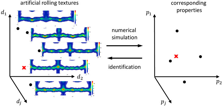
FIGURE 6. Illustration of the texture identification problem. The space of rolling textures is described by dj and the space of properties by pj.
In Iraki et al. (2021), texture generation is done based on the rolling texture description model described in Delannay et al. (1999). In this study, the parameter ranges for the texture description model are defined as is described in Iraki et al. (2021). To calculate the properties of interest, a crystal plasticity model is used. The model is of Taylor-type and is set up following Kalidindi et al. (1992). For a detailed description of the Taylor-type crystal plasticity model, see Dornheim et al. (2022) and Iraki et al. (2021). Besides, instead of using a Taylor-type crystal plasticity model, also computationally expensive full-field models can be applied here. For the purpose of our study, we use the Taylor-type crystal plasticity model to determine the Young’s moduli Eφ and the Lankford coefficients (r-values) rφ, both at 0, 45 and 90° to rolling direction for given crystallographic textures. In the following, the generated properties are represented by
In the following, we compare the generation of 5,000 texture-property data pairs using Latin hypercube design and query-by-committee. As r-values of rolled DC04 sheets typically do not exceed values of 5.0, we additionally apply the extension described in Section 2.2 to suppress generating data in regions leading to r > 5.0 (the factor to weight the soft constraint W in Eq. 5 is set to 100). For the query-by-committee approach, a committee of five neural networks is used with two hidden layers of 24 and 6 neurons. Every committee member is trained on a random subset of 80% of the actual data. The mean-squared-error loss function between true and predicted properties is applied and the limited-memory BFGS optimizer is used. Early stopping and L2-regularization with λ = 0.1 are applied. The activation function used is ReLU. For an initial data set, 100 texture-property data points are sampled randomly.
The obtained data sets are depicted as projections in property space in Figure 7 (E0, E90) and Figure 8 (r45, r0). The point cloud generated by Latin hypercube design comprises a much smaller region in property space compared to the ones generated by query-by-committee. Furthermore, the point cloud is concentrated at its center. Such a strong concentration cannot be observed in the point clouds generated by query-by-committee. Also the minimum and maximum values in both, E and r, that are found by the active learning strategies are more extreme than by using Latin hypercube design. However, the original query-by-committee sampling approach leads to unrealistic high r-values, cf. Figure 8B. In contrast, Figure 8C shows that this effect can be minimized by applying the extension to query-by-committee presented in Section 2.2. The applied region filter (isolation forest) limits the active learning search space in such a way that textures with high r-values are excluded. Therefore, the amount of textures in the data set that lead to unrealistic high r-values decreases dramatically compared to the data set generated without the query-by-committee extension. The latter includes 141 data points with r > 5, while the former includes only 11. The generated data is available online, see Morand et al. (2021).

FIGURE 7. 5,000 sampled texture-property data points projected into property space (E0, E90). Data points are generated on the basis of Latin hypercube design (A), query-by-committee (B) and extended query-by-committee with r ≤ 5.0 (C).

FIGURE 8. 5,000 sampled texture-property data points projected into property space (r45, r0). The data points are generated on the basis of Latin hypercube design (A), query-by-committee (B) and extended query-by-committee with r ≤ 5.0 (C).
To evaluate the effect of the applied sampling strategies on supervised learning models, we train and test feedforward neural networks on the generated data. For training and testing, we exclude the data points with r > 5.0. In contrast to Section 3.2, only the forward mapping is modeled, as the inverse relation cannot be learned directly using feedforward neural networks due to its non-uniqueness. For the forward mapping, first, we approximate the orientation distribution function of the generated textures via symmetric generalized spherical harmonics of degree 12 Bunge (2013). The constants
where
The performance measure for the neural networks used in this example is the mean absolute error for the Young’s moduli
and for the r-values
Table 2 and 3 show the results of the trained neural networks, when tested on the generated data. Training and test runs were performed five times with different random validation splits. The mean and maximum errors were averaged over the data set. Both tables show that the neural networks trained with data generated by query-by-committee outperform the neural networks trained with data generated on the basis of Latin hypercube design. However, the differences in the averaged mean errors are not significantly high. In contrast, regarding the averaged maximum errors, the differences are much higher. When tested on the data set generated by Latin hypercube design, both neural networks that are trained with data generated by query-by-committee achieve similar results.
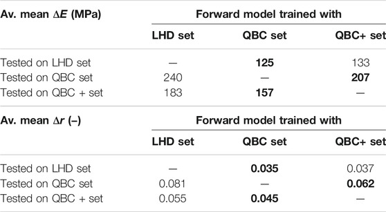
TABLE 2. Average mean ΔE and Δr for the neural networks trained and evaluated on the three generated data sets: LHD (Latin hypercube design), QBC (query-by-committee) and QBC+ (query-by-committee with extension). The best result for each test set is marked in bold.
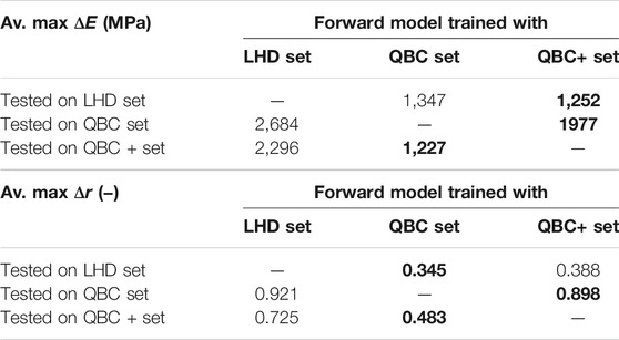
TABLE 3. Average maximum ΔE and Δr for the neural networks trained and evaluated on the three generated data sets: LHD (Latin hypercube design), QBC (query-by-committee) and QBC+ (query-by-committee with extension). The best result for each test set is marked in bold.
4 Discussion
In Section 3.1, an extreme case is studied to emphasize the advantage of using active learning for the generation of microstructure-property data sets. The peak of the approximated delta function is chosen to be quite steep such that the probability of sampling data points on it by random sampling is rather small. As a result, random sampling covers the peak region of the delta function insufficiently. In contrast, by using query-by-committee, the peak region is explored extensively. As pointed out, even the maximum value in the sampled data set is very close to the maximum value of the approximated delta function. If we imagine the delta function expressing a relation between microstructures and properties, we can easily see the advantage for a designer to gain knowledge about the property peak in order to be able to improve the performance of a workpiece.
In Section 3.2, the query-by-committee approach is compared to a classical Latin hypercube design approach and a knowledge-based sampling approach for generating data of hardening model parameters and responses. Originally, the knowledge-based approach was developed in Morand and Helm (2019) to optimally sample the hardening model’s parameter space by incorporating knowledge about the model’s behavior. The results show that the query-by-committee approach is able to find a similar parameter distribution, but without manually introducing any expert knowledge. The data generated by query-by-committee is equally appropriate for training forward and inverse neural network models, which all outperform the models trained on the data generated by the baseline Latin hypercube design approach. All in all, the results show that by using query-by-committee, sampling can be performed automatically in a goal-directed way without additionally introducing expert knowledge.
Also, the results from Section 3.3 show that the query-by-committee approach is more suitable to sample microstructure-property spaces than classical space-filling sampling strategies. In this example, a space of artificial rolling textures is sampled aiming to efficiently explore the space of corresponding properties. A comparison of the spread of the generated properties point clouds reveals with which additional possibilities a designer can be equipped, when the design space is sampled via active learning. However, the original query-by-committee approach explores the texture space in regions that lead to unrealistic high properties. By using the extension to membership query synthesis that is presented in this paper, sampling in regions with unrealistic high properties can be suppressed. In fact, still some data points are generated in these regions, which are yet necessary for the binary classifier (region filter) to be trained. Nevertheless, compared to the classical query-by-committee approach, the amount of property data out of scope is much lower and sampling concentrates on the predefined region of interest. Consequently, when training a supervised learning model on the inverse relation (predicting textures for given properties), more extreme properties can be learned on the basis of data generated by query-by-committee.
Such a positive effect can also be observed on learning the forward relation. The neural networks trained on the data generated by query-by-committee both outperform the model trained with the data generated by Latin hypercube design. However, no significant differences in the averaged mean absolute error (shown in Table 2) can be seen. This is due to the fact that most of the data points are located near the center of the point cloud, which is where all the neural networks are quite accurate. In contrast, the differences in the averaged maximum errors are more significant. This is because the data sets sampled by query-by-committee contains more extreme data points than the data set sampled by Latin hypercube design. Furthermore, it can be seen that the neural network trained on the data generated by the extended query-by-committee approach performs worse than the network trained with the data from the original approach. This is a sign that the region filter limits the texture space too rigorously and further adjustment is needed. However, the general concept of the active learning extension is proven, as less samples were generated in regions out of scope compared to the original approach.
5 Summary and Outlook
The present paper shows that active learning can be used to efficiently explore microstructure-property spaces. By using the active learning approach query-by-committee, the focus of data generation is automatically shifted to sparse regions and nonlinearities. Subsequently, two main advantages of active learning in materials design applications follow: 1) regions in microstructure space that lead to extreme properties are explored extensively and 2) in contrast to classical space-filling sampling strategies, active learning can be used for goal-directed sampling, which is relevant for training direct inverse machine learning models. Future work is, however, necessary to investigate how the size of the committee, the fraction of the data used to train the committee members and the complexity of these affect sampling. Also it is necessary to benchmark the query-by-committee approach to the Bayesian approaches, which are mentioned in the introduction.
In general, a problem for active learning approaches arises, when the input space bounds are not set adequately. Then, regions in microstructure space are explored that lead to properties out of scope. However, sampling in these regions can be suppressed by using the extension presented in this work. Still one drawback of using active learning remains: In contrast to classical sampling strategies, active learning is time-intensive, as in every active learning cycle one or more machine learning models need to be trained and additionally an optimization has to be performed. Yet, the results of the present paper show that by using active learning, less data is needed to sufficiently cover microstructure-property spaces than it is the case for classical sampling strategies.
Therefore, regarding virtual materials design, the application of active learning techniques is suitable when sample-efficiency plays an important role. This is for example the case when data is generated using time-intensive numerical simulations, like for example on the bases of spatially resolved full-field microstructures. Also, active learning can help setting up multi-fidelity data bases by enriching less quality data with precisely sampled high quality simulation data or experimental data. Though, incorporating multi-fidelity data and experimental data has not been studied in this work and is part of future research.
Data Availability Statement
The data sets generated for this study can be found in the Fraunhofer Fordatis repository at https://fordatis.fraunhofer.de/handle/fordatis/219, see Morand et al. (2021).
Author Contributions
LM set up the active learning framework, developed the extension to membership query synthesis with a region filter, generated the results and wrote the manuscript. NL had the idea to develop the extension to membership query synthesis. TI, JD, and NL supported in terms of machine learning and helped fundamentally by discussing the approach. DH supported in terms of materials sciences and modeling. All authors contributed to the discussion of the results and to the summary and outlook.
Conflict of Interest
The authors declare that the research was conducted in the absence of any commercial or financial relationships that could be construed as a potential conflict of interest.
Publisher’s Note
All claims expressed in this article are solely those of the authors and do not necessarily represent those of their affiliated organizations, or those of the publisher, the editors and the reviewers. Any product that may be evaluated in this article, or claim that may be made by its manufacturer, is not guaranteed or endorsed by the publisher.
Acknowledgments
The authors would like to thank the German Research Foundation (DFG) for funding this work, which was carried out within the research project number 415 804 944: “Taylored Material Properties via Microstructure Optimization: Machine Learning for Modelling and Inversion of Structure-Property-Relationships and the Application to Sheet Metals”.
References
Adams, B. L., Henrie, A., Henrie, B., Lyon, M., Kalidindi, S. R., and Garmestani, H. (2001). Microstructure-Sensitive Design of a Compliant Beam. J. Mech. Phys. Sol. 49, 1639–1663. doi:10.1016/s0022-5096(01)00016-3
Balachandran, P. V., Xue, D., Theiler, J., Hogden, J., and Lookman, T. (2016). Adaptive Strategies for Materials Design Using Uncertainties. Sci. Rep. 6 19660–19669. doi:10.1038/srep19660
Bessa, M. A., Bostanabad, R., Liu, Z., Hu, A., Apley, D. W., Brinson, C., et al. (2017). A Framework for Data-Driven Analysis of Materials under Uncertainty: Countering the Curse of Dimensionality. Comput. Methods Appl. Mech. Eng. 320, 633–667. doi:10.1016/j.cma.2017.03.037
Bunge, H.-J. (2013). Texture Analysis in Materials Science: Mathematical Methods. Burlington: Elsevier Science.
Burbidge, R., Rowland, J. J., and King, R. D. (2007). “Active Learning for Regression Based on Query by Committee,” in Proceeding of the Intelligent Data Engineering and Automated Learning - IDEAL 2007, 8th International Conference Berlin, Heidelberg: Springer, December 16-19, 2007, 209–218. doi:10.1007/978-3-540-77226-2_22
Cai, W., Zhang, Y., and Zhou, J. (2013). “Maximizing Expected Model Change for Active Learning in Regression,” in Proceeding of the IEEE 13th International Conference on Data Mining, Dallas, TX, USA, 7-10 Dec. 2013 (IEEE), 51–60. doi:10.1109/ICDM.2013.104
Castillo, A. R., Joseph, V. R., and Kalidindi, S. R. (2019). Bayesian Sequential Design of Experiments for Extraction of Single-crystal Material Properties from Spherical Indentation Measurements on Polycrystalline Samples. JOM 71, 2671–2679. doi:10.1007/s11837-019-03549-x
Chalapathy, R., and Chawla, S. (2019). Deep Learning for Anomaly Detection: A Survey. arXiv: 1901.03407 preprint.
Cohn, D. A., Ghahramani, Z., and Jordan, M. I. (1996). Active Learning with Statistical Models. JAIR 4, 129–145. doi:10.1613/jair.295
Delannay, L., Van Houtte, P., and Van Bael, A. (1999). New Parameter Model for Texture Description in Steel Sheets. Textures and Microstructures 31, 151–175. doi:10.1155/tsm.31.151
Dornheim, J., Morand, L., Zeitvogel, S., Iraki, T., Link, N., and Helm, D. (2022). Deep Reinforcement Learning Methods for Structure-Guided Processing Path Optimization. J. Intell. Manufacturing 33, 333–352. doi:10.1007/s10845-021-01805-z
Eghtesad, A., and Knezevic, M. (2020). High-performance Full-Field Crystal Plasticity with Dislocation-Based Hardening and Slip System Back-Stress Laws: Application to Modeling Deformation of Dual-phase Steels. J. Mech. Phys. Sol. 134, 103750. doi:10.1016/j.jmps.2019.103750
Fang, K.-T., Lin, D. K. J., Winker, P., and Zhang, Y. (2000). Uniform Design: Theory and Application. Technometrics 42, 237–248. doi:10.1080/00401706.2000.10486045
Forrester, A. I. J., and Keane, A. J. (2009). Recent Advances in Surrogate-Based Optimization. Prog. Aerospace Sci. 45, 50–79. doi:10.1016/j.paerosci.2008.11.001
Fullwood, D. T., Niezgoda, S. R., Adams, B. L., and Kalidindi, S. R. (2010). Microstructure Sensitive Design for Performance Optimization. Prog. Mater. Sci. 55, 477–562. doi:10.1016/j.pmatsci.2009.08.002
Gupta, A., Cecen, A., Goyal, S., Singh, A. K., and Kalidindi, S. R. (2015). Structure-property Linkages Using a Data Science Approach: Application to a Non-metallic Inclusion/steel Composite System. Acta. Mater. 91, 239–254. doi:10.1016/j.actamat.2015.02.045
Halton, J. H. (1964). Algorithm 247: Radical-Inverse Quasi-Random point Sequence. Commun. ACM 7, 701–702. doi:10.1145/355588.365104
Heese, R., Walczak, M., Seidel, T., Asprion, N., and Bortz, M. (2019). Optimized Data Exploration Applied to the Simulation of a Chemical Process. Comput. Chem. Eng. 124, 326–342. doi:10.1016/j.compchemeng.2019.01.007
Helm, D. (2006). Stress Computation in Finite Thermoviscoplasticity. Int. J. Plasticity 22, 1699–1727. doi:10.1016/j.ijplas.2006.02.007
Hinton, G. E., and Salakhutdinov, R. R. (2006). Reducing the Dimensionality of Data with Neural Networks. Science 313, 504–507. doi:10.1126/science.1127647
Huber, N. (2000). Anwendung neuronaler Netze bei nichtlinearen Problemen der Mechanik: Karlsruhe FZKA 2000. Tech. rep., Forschungszentrum Karlsruhe Technik und Umwelt. Habilitation thesis German.
Huber, N., and Tsakmakis, C. (1999). Determination of Constitutive Properties from Spherical Indentation Data Using Neural Networks. Part I: The Case of Pure Kinematic Hardening in Plasticity Laws. J. Mech. Phys. Sol. 47, 1569–1588. doi:10.1016/s0022-5096(98)00109-4
Iraki, T., Morand, L., Dornheim, J., Link, N., and Helm, D. (2021). A Multi-Task Learning-Based Optimization Approach for Finding Diverse Sets of Material Microstructures with Desired Properties and its Application to Texture Optimization. arXiv:2111.00916.
Johnson, O. K., and Kurniawan, C. (2018). An Efficient Algorithm for Generating Diverse Microstructure Sets and Delineating Properties Closures. Acta. Mater. 147, 313–321. doi:10.1016/j.actamat.2018.01.004
Jordan, M. I., and Rumelhart, D. E. (1992). Forward Models: Supervised Learning with a Distal Teacher. Cogn. Sci. 16, 307–354. doi:10.1207/s15516709cog1603_1
Jung, J., Yoon, J. I., Park, H. K., Kim, J. Y., and Kim, H. S. (2019). An Efficient Machine Learning Approach to Establish Structure-Property Linkages. Comput. Mater. Sci. 156, 17–25. doi:10.1016/j.commatsci.2018.09.034
Kalidindi, S. R. (2019). A Bayesian Framework for Materials Knowledge Systems. MRS Commun. 9, 518–531. doi:10.1557/mrc.2019.56
Kalidindi, S. R., Bronkhorst, C. A., and Anand, L. (1992). Crystallographic Texture Evolution in Bulk Deformation Processing of FCC Metals. J. Mech. Phys. Sol. 40, 537–569. doi:10.1016/0022-5096(92)80003-9
Kalidindi, S. R., Houskamp, J. R., Lyons, M., and Adams, B. L. (2004). Microstructure Sensitive Design of an Orthotropic Plate Subjected to Tensile Load. Int. J. Plasticity 20, 1561–1575. doi:10.1016/j.ijplas.2003.11.007
Krogh, A., and Hertz, J. A. (1992). “A Simple Weight Decay Can Improve Generalization,” in Advances in Neural Information Processing Systems Denver, 950–957. doi:10.5555/2998687.2998716
Krogh, A., and Vedelsby, J. (1995). Neural Network Ensembles, Cross Validation, and Active Learning. Adv. Neural Inf. Process. Syst. 7, 231–238.
Liu, D. C., and Nocedal, J. (1989). On the Limited Memory BFGS Method for Large Scale Optimization. Math. programming 45, 503–528. doi:10.1007/bf01589116
Liu, F. T., Ting, K. M., and Zhou, Z.-H. (2008). “Isolation forest,” in 8th IEEE International Conference on Data Mining. Pisa, Italy: IEEE Xplore, 413–422. doi:10.1109/icdm.2008.17
Liu, R., Kumar, A., Chen, Z., Agrawal, A., Sundararaghavan, V., and Choudhary, A. (2015a). A Predictive Machine Learning Approach for Microstructure Optimization and Materials Design. Sci. Rep. 5, 11551–11612. doi:10.1038/srep11551
Liu, R., Yabansu, Y. C., Agrawal, A., Kalidindi, S. R., and Choudhary, A. N. (2015b). Machine Learning Approaches for Elastic Localization Linkages in High-Contrast Composite Materials. Integr. Mater. Manuf. 4, 192–208. doi:10.1186/s40192-015-0042-z
Lookman, T., Balachandran, P. V., Xue, D., Hogden, J., and Theiler, J. (2017). Statistical Inference and Adaptive Design for Materials Discovery. Curr. Opin. Solid State. Mater. Sci. 21, 121–128. doi:10.1016/j.cossms.2016.10.002
Lookman, T., Balachandran, P. V., Xue, D., and Yuan, R. (2019). Active Learning in Materials Science with Emphasis on Adaptive Sampling Using Uncertainties for Targeted Design. npj Comput. Mater. 5, 1–17. doi:10.1038/s41524-019-0153-8
Mahnken, R. (2004). Identification of Material Parameters for Constitutive Equations. New York: John Wiley & Sons. chap. 19. 637–655.
Mayer, C., and Timofte, R. (2020). “Adversarial Sampling for Active Learning,” in Proceedings of the IEEE/CVF Winter Conference on Applications of Computer Vision, Snowmass, CO, USA, 1-5 March 2020 (IEEE), 3071–3079. doi:10.1109/WACV45572.2020.9093556
McKay, M. D., Beckman, R. J., and Conover, W. J. (2000). A Comparison of Three Methods for Selecting Values of Input Variables in the Analysis of Output from a Computer Code. Technometrics 42, 55–61. doi:10.1080/00401706.2000.10485979
Morand, L., and Helm, D. (2019). A Mixture of Experts Approach to Handle Ambiguities in Parameter Identification Problems in Material Modeling. Comput. Mater. Sci. 167, 85–91. doi:10.1016/j.commatsci.2019.04.003
Morand, L., Iraki, T., Dornheim, J., Link, N., and Helm, D. (2021). Sets of Exemplary Microstructure-Property Data Generated via Active Learning and Numerical Simulations - Fraunhofer Fordatis Repository. Available at: https://fordatis.fraunhofer.de/handle/fordatis/219.
Niederreiter, H. (1988). Low-discrepancy and Low-Dispersion Sequences. J. Number Theor. 30, 51–70. doi:10.1016/0022-314x(88)90025-x
Nikolaev, P., Hooper, D., Webber, F., Rao, R., Decker, K., Krein, M., et al. (2016). Autonomy in Materials Research: a Case Study in Carbon Nanotube Growth. npj Comput. Mater. 2, 1–6. doi:10.1038/npjcompumats.2016.31
Owen, A. B. (1992). Orthogonal Arrays for Computer Experiments, Integration and Visualization. Stat. Sinica 2, 439–452.
Paul, A., Acar, P., Liao, W.-k., Choudhary, A., Sundararaghavan, V., and Agrawal, A. (2019). Microstructure Optimization with Constrained Design Objectives Using Machine Learning-Based Feedback-Aware Data-Generation. Comput. Mater. Sci. 160, 334–351. doi:10.1016/j.commatsci.2019.01.015
Pedregosa, F., Varoquaux, G., Gramfort, A., Michel, V., Thirion, B., Grisel, O., et al. (2011). Scikit-learn: Machine Learning in Python. J. Machine Learn. Res. 12, 2825–2830. doi:10.5555/1953048.2078195
Prechelt, L. (1998). “Early Stopping - but when?” in Neural Networks: Tricks of the Trade (Berlin, Heidelberg: Springer), 55–69. doi:10.1007/3-540-49430-8_3
RayChaudhuri, T., and Hamey, L. G. C. (1995). “Minimisation of Data Collection by Active Learning,” in Proceedings of ICNN’95 - International Conference on Neural Networks, Perth, WA, Australia, 27 Nov.-1 Dec. 1995 (IEEE), 1338–1341. doi:10.1109/ICNN.1995.487351
Sacher, M., Duvigneau, R., Le Maître, O., Durand, M., Berrini, É., Hauville, F., et al. (2018). A Classification Approach to Efficient Global Optimization in Presence of Non-computable Domains. Struct. Multidisc. Optim. 58, 1537–1557. doi:10.1007/s00158-018-1981-8
Sakurada, M., and Yairi, T. (2014). “Anomaly Detection Using Autoencoders with Nonlinear Dimensionality Reduction,” in Proceedings of the MLSDA 2014 2nd Workshop on Machine Learning for Sensory Data Analysis. Gold Coast: Association for Computing Machinery, 4–11. doi:10.1145/2689746.2689747
Sambu Seo, S., Wallat, M., Graepel, T., and Obermayer, K. (2000). “Gaussian Process Regression: Active Data Selection and Test Point Rejection,” in Proceedings of the IEEE-INNS-ENNS International Joint Conference on Neural Networks - IJCNN 2000, Como, Italy, 27-27 July 2000. doi:10.1109/IJCNN.2000.861310
Schölkopf, B., Platt, J. C., Shawe-Taylor, J., Smola, A. J., and Williamson, R. C. (2001). Estimating the Support of a High-Dimensional Distribution. Neural Comput. 13, 1443–1471. doi:10.1162/089976601750264965
Settles, B. (2012). Active Learning. Synth. Lectures Artif. Intelligence Machine Learn. 6, 1–114. doi:10.2200/s00429ed1v01y201207aim018
Settles, B. (2009). Active Learning Literature Survey. 1648. Tech. rep. Madison, Wisconsin: University of Wisconsin–Madison, Department of Computer Science.
Seung, H. S., Opper, M., and Sompolinsky, H. (1992). “Query by Committee,” in Proceedings of the Fifth Annual Workshop on Computational Learning Theory. Pittsburgh: Association for Computing Machinery, 287–294. doi:10.1145/130385.130417
Simpson, T. W., Lin, D. K., and Chen, W. (2001). Sampling Strategies for Computer Experiments: Design and Analysis. Int. J. Reliability Appl. 2, 209–240.
Sinha, S., Ebrahimi, S., and Darrell, T. (2019). “Variational Adversarial Active Learning,” in Proceedings of the IEEE/CVF International Conference on Computer Vision. Seoul: IEEE Xplore, 5972–5981. doi:10.1109/iccv.2019.00607
Sobol, I. M. (1967). On the Distribution of Points in a Cube and the Approximate Evaluation of Integrals. USSR Comput. Mathematics Math. Phys. 7, 86–112. doi:10.1016/0041-5553(67)90144-9
Stark, F., Hazırbas, C., Triebel, R., and Cremers, D. (2015). “Captcha Recognition with Active Deep Learning,” in Workshop New Challenges in Neural Computation 2015, 94.
Storn, R., and Price, K. (1997). Differential Evolution – a Simple and Efficient Heuristic for Global Optimization over Continuous Spaces. J. Glob. Optimization 11, 341–359. doi:10.1023/a:1008202821328
Tang, B. (1993). Orthogonal Array-Based Latin Hypercubes. J. Am. Stat. Assoc. 88, 1392–1397. doi:10.1080/01621459.1993.10476423
Tran, A., Sun, J., Furlan, J. M., Pagalthivarthi, K. V., Visintainer, R. J., and Wang, Y. (2019). pBO-2GP-3B: A Batch Parallel Known/unknown Constrained Bayesian Optimization with Feasibility Classification and its Applications in Computational Fluid Dynamics. Comput. Methods Appl. Mech. Eng. 347, 827–852. doi:10.1016/j.cma.2018.12.033
Tran, A., and Wildey, T. (2021). Solving Stochastic Inverse Problems for Property-Structure Linkages Using Data-Consistent Inversion and Machine Learning. JOM 73, 72–89. doi:10.1007/s11837-020-04432-w
Virtanen, P., Gommers, R., Oliphant, T. E., Haberland, M., Reddy, T., Cournapeau, D., et al. (2020). SciPy 1.0: Fundamental Algorithms for Scientific Computing in Python. Nat. Methods 17, 261–272. doi:10.1038/s41592-019-0686-2
Wang, G. G., and Shan, S. (2006). Review of Metamodeling Techniques in Support of Engineering Design Optimization. J. Mech. Des. 129, 370–380. doi:10.1115/1.2429697
Wang, K., Zhang, D., Li, Y., Zhang, R., and Lin, L. (2016). Cost-effective Active Learning for Deep Image Classification. IEEE Trans. Circuits Syst. Video Technology 27, 2591–2600. doi:10.1109/TCSVT.2016.2589879
Williams, C. K., and Rasmussen, C. E. (2006). Gaussian Processes for Machine Learning. Vol. 2. Cambridge, MA: MIT press.
Yagawa, G., and Okuda, H. (1996). Neural Networks in Computational Mechanics. Arch. Comput. Methods Eng. 3, 435–512. doi:10.1007/bf02818935
Keywords: active learning, adaptive sampling, data generation, inverse modeling, materials design, membership query synthesis, microstructure-property relations, query-by-committee
Citation: Morand L, Link N, Iraki T, Dornheim J and Helm D (2022) Efficient Exploration of Microstructure-Property Spaces via Active Learning. Front. Mater. 8:824441. doi: 10.3389/fmats.2021.824441
Received: 29 November 2021; Accepted: 22 December 2021;
Published: 14 February 2022.
Edited by:
Surya R. Kalidindi, Georgia Institute of Technology, United StatesReviewed by:
Anh Tran, Sandia National Laboratories, United StatesTomasz Michno, Kielce University of Technology, Poland
Copyright © 2022 Morand, Link, Iraki, Dornheim and Helm. This is an open-access article distributed under the terms of the Creative Commons Attribution License (CC BY). The use, distribution or reproduction in other forums is permitted, provided the original author(s) and the copyright owner(s) are credited and that the original publication in this journal is cited, in accordance with accepted academic practice. No use, distribution or reproduction is permitted which does not comply with these terms.
*Correspondence: Lukas Morand, bHVrYXMubW9yYW5kQGl3bS5mcmF1bmhvZmVyLmRl
 Lukas Morand
 Norbert Link2
 Johannes Dornheim
 Dirk Helm