Micro-Scale Permeability Characterization of Carbon Fiber Composites Using Micrograph Volume Elements

To manufacture a high-performance structure made of continuous fiber reinforced plastics, Liquid Composite Molding processes are used, where a liquid resin infiltrates the dry fibers. For a good infiltration quality without dry spots, it is important to predict the resin flow correctly. Knowledge of the local permeability is an essential precondition for mold-filling simulations. In our approach, the intra-bundle permeability parallel and transverse to the fibers is characterized via periodic fluid dynamic simulations of micro-scale volume elements (VE). We evaluate and compare two approaches: First, an approach to generate VEs based on a statistical distribution of the fibers and fiber diameters. Second, an approach based on micrograph images of samples manufactured with Tailored Fiber Placement (TFP) using the measured fiber distribution. The micrograph images show a higher heterogeneity of the distribution than the statistically generated VEs, which is characterized by large resin areas. This heterogeneity leads to a significantly different permeability compared to the stochastic approach. In conclusion, a pure stochastic approach needs to contain the large heterogeneity of the fiber distribution to predict correct permeability values.

Introduction

In high-performance lightweight design, engineers often choose continuous fiber reinforced plastics (CoFRP) as structural material because of their very high specific mechanical properties (Henning et al., 2019). Especially carbon fiber reinforced plastics exhibit outstanding weight specific strength and stiffness. In Tailored Fiber Placement (TFP), dry carbon fiber rovings are stitched onto a base material to form a variable-axial preform (Mattheij et al., 1998). Variable-axial TFP enables to produce parts with arbitrary fiber orientation and, furthermore, to optimize their strength and stiffness (Spickenheuer et al., 2008; Bittrich et al., 2019). One possibility to produce CoFRP from these preforms is to infiltrate the dry fibers with a liquid resin and a following curing of the resin under application of heat and pressure. Those kind of manufacturing processes are often referred to as Liquid Composite Molding and can be divided into several process routes, e.g. Resin Transfer Molding (RTM) or Wet Compression Molding (Seuffert et al., 2020; Poppe et al., 2021).

One important aspect during manufacturing is the infiltration behavior of the fibers (Kärger et al., 2015). On a macro-scale, the wetting of the fibers is characterized as a flow inside a porous medium where the fibers induce a drag force against the liquid resin. This drag force is captured by the material parameter permeability. With this parameter, the pressure-velocity relationship in a porous medium is given by the well-known Darcy equation (Darcy, 1856):

$\tilde{\mathit{v}}=-\frac{\mathit{K}}{\mu }\mathrm{\nabla }p$

with the volume-averaged fluid velocity $\tilde{\mathit{v}}$, the viscosity $\mu$, the pressure gradient $\mathrm{\nabla }p$ and the permeability $\mathit{K}$. A lot of effort is put into the experimental characterization of in-plane and out-of-plane permeability on macro-scale (Arbter et al., 2011; Vernet et al., 2014; Magagnato and Henning 2015; May et al., 2019; Yong et al., 2021). As the experimental cost is high, also attempts to characterize the permeability based on analytical, empirical or numerical methods are made. It was shown that the permeability on macro-scale depends on micro-scale and meso-scale geometric structures, which is the flow between the fibers inside a roving and the flow between the rovings, respectively. An analytical and empirical investigation is based mainly on the work of Kozeny (1927) and Carman (1937) for spherical particles and an extension to cylindrical particles by Gebart (1992). Gebart used a regular system of fibers in a square or hexagonal arrangement, which is a strong simplification of the real fiber network as shown in many following studies.

Gommer et al. (2016) analyzed the micro-scale fiber arrangement of a plain weave fabric using micrographs. They showed that the local fiber volume fraction varies significantly inside a roving, which can lead to local air entrapments or resin-rich channels. Um and Lee (1997) analyzed the flow based on micrograph images by generating a network model of the fiber arrangement, calculating the Kozeny constant (which is a function of fiber volume fraction and the amount of heterogeneity of the arrangement (Åström et al., 1992)), and comparing it to analytical solution and experimental results. They concluded that the non-uniform fiber arrangement is better suited to predict the real permeability in a fibrous network, which was also shown by Cai and Berdychevsky (1993). This led to several distribution approaches that were used to better include this fact. Bechtold and Ye (2003) analyzed different distribution patterns using a stochastic model and showed that the amount of randomness influences the permeability, as sometimes large channels are formed, whereas some other channels can be blocked. However, the stochastic model only contained 15 fibers, which limits the validity of the stochastic model. Chen and Papathanasiou (2007), Chen and Papathanasiou (2008) used a Monte-Carlo method to randomly distribute fibers in a representative volume. They analyzed the stochastic properties with the nearest inter fiber spacing that correlates with axial and transverse permeability, which was also reported by Matsumura and Jackson (2014). They summarized, that a statistical measure of the fiber arrangement is needed additionally to the fiber volume fraction for a more realistic permeability model. In their simulation model, they use no-slip wall boundary conditions at the edges of the non-periodic model, which lead to a significant size effect, that is significant when using less than 100 fibers. Endruweit et al. (2013) applied the Gebart model to micrographs by assuming that the fiber arrangement can be interpreted as a network of hexagonal or square arrangements in series and parallel. They indicate that the axial permeability is higher than the analytic description by Gebart, because axial permeability is dominated by large fiber gaps (low local fiber volume fraction). In the case of transverse permeability, they calculate lower permeabilities for lower fiber volume fractions compared to the results using Gebart’s equations. For the case of high fiber volume fraction, their values lie between the results using square and hexagonal arrangements. Rimmel and May (2020) concluded that a minimum of 10 simulations is necessary to capture the Gaussian distribution of the permeabilities for one fiber volume fraction. They also analyzed the influence of different boundary condition types but without ensuring periodicity at the edges of the micro-scale elements, which makes a comparison to periodic models difficult. Gommer et al. (2018) pointed out that the nearest fiber distance does not influence the permeability as strong as the distance towards the second and third nearest neighbor, which was also the result by investigations of Yazdchi et al. (2012). Yazdchi and Luding (2013) also used Delaunay triangulations and Voronoi polygons to deduce necessary information to characterize the fiber arrangements at micro-scale, though they focused on pure numerical investigations without comparison to real CoFRP fiber distributions. Recently, Zarandi et al. (2019) compared many different theoretical methods to simulations with random fiber distribution and roving-sized permeability measurements. They pointed out that the fiber clustering generated through random distribution is important and should be considered in permeability models. Their numerical VE was comparably small (about six times the fiber diameter) and thus cannot show any influence of larger gaps onto the permeability. Furthermore, it is not clear, if the fiber distribution inside a roving in a manually made specimen containing only one roving is equal to the fiber distribution inside a real manufactured component.

The publications indicate, that the stochastic distribution of the fibers inside a roving plays an important role to predict the intra-roving permeability. These conclusions are based on numerical and analytical models. No direct comparison of the stochastic fiber arrangement and the real fiber arrangement in a roving was made to directly show the resulting differences in micro-scale permeability. In our work, we therefore on the one hand use a numerical stochastic approach to generate statistical volume elements (SVE) and on the second hand we use micrograph images of samples manufactured via RTM to generate periodic micrograph volume elements (MVE). We compare statistical parameters of both approaches and show their influence on the micro-scale permeability, which allows for a more realistic micro-scale modeling in the future.

Fiber Distribution and Modeling on Micro-Scale

Evaluation of the Fiber Distribution on Micro-Scale

The analysis of the fiber distribution on micro-scale is based on micrographs that are made from manufactured TFP plates made of unidirectional rovings. The infiltration of the TFP plates is achieved using an RTM process with carbon fiber rovings (HTS45 - 12K) from Toho Tenax GmbH. The micrographs were made using Keyence VHX-2000 digital multi-scan microscope. Figure 1 shows two micrograph images used in the analysis. In total, 36 micrograph images are used with a magnification of 700× with 0.29 µm / pixel. The images are analyses using a cascade of steps with the OpenCV image library (Bradski, 2000) that is visualized in Figure 2. The image data (A) is denoised by a Gaussian blur of radius 3 pixels (B). Next, an adaptive Gaussian threshold is applied to consider non-uniform lighting in the images (C). Using a morphological transformation, a sure foreground is obtained by an opening transformation with uniform 3 × 3 kernels (D) and a threshold on its Laplacian distance transformation to find centers of local clusters (E). This procedure is meant to separate all filaments that touch each other and thus form continuous areas. The opening transformation itself is shrinking these areas already and the distance transformation yields pixel values of the closest distance to the boundary. Two or more touching fibers will then form distinct local maxima that can be separated by thresholding. The contours of the resulting binary image are evaluated for their center positions (see red contours in Figure 2F with center positions in black), which closely resemble the fiber center positions.

FIGURE 1

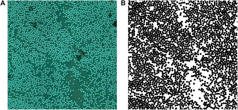
FIGURE 1. (A) Micrograph of a carbon fiber roving, transverse to main fiber orientation; Fibers show brighter compared to the epoxy resin; (B) Representation of the micrograph after applying the fiber detection algorithm; large pure resin areas are visible in the right half of the images in white color.

FIGURE 2

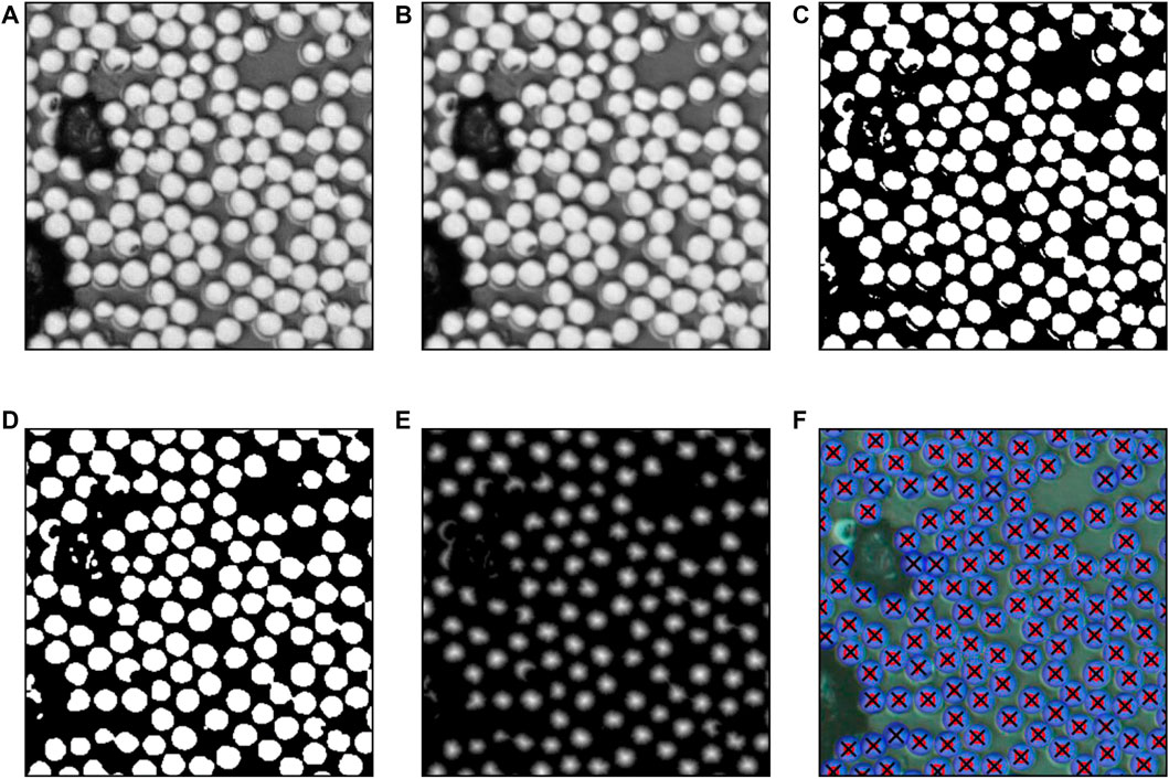
FIGURE 2. Sequence of image analysis steps to find the fiber filament center positions in micrograph images. The original gray scale image is shown in (A) and minimal noise is filtered by blurring (B). A Gaussian adaptive threshold gives a black and white contrast (C). Small artefacts are removed by an opening transformation (D) and a Laplacian distance transform is obtained in (E). A normal thresholding of this distance transform yields the red contours in (F) superimposed on the original image with the center positions in black and blue semitransparent circles of radius 7 µm.

The diameter of the fibers is not determined with these images due to the limited resolution and blurring at the boundaries. Instead, a mean fiber diameter $\overline{D}$ of 7 µm based on the material data sheet is assumed with a standard deviation ${\sigma }_D$ of the diameter of 0.45 µm.

Generation of Micro-Scale Volume Elements Based on Micrographs and Statistical Distributions

Based on the fiber coordinates, a statistical analysis of the fiber arrangement is conducted. To compare and analyze the arrangements, we use a Delaunay-triangulation of the fiber coordinates. In a second step we calculate the areas of the Voronoi-polygons based on this triangulation. A large Voronoi-polygon area signifies a larger space to neighboring fibers and therefore is a quantitative representation of a low local fiber density. The standard deviations of the Voronoi-polygon areas are thus a quantitative measurement of the heterogeneity of the fiber arrangement. The Voronoi-polygon areas are normalized with the mean Voronoi-polygon area at the present fiber volume fraction of the micrograph, so assuming a perfect homogeneity. This allows us to compare only the relative area sizes and deviations independently of the fiber volume fraction.

Figure 3 shows the Voronoi polygons for the micrograph of Figure 1. The large inter-fiber gaps visible in the lower part of the micrograph are visualized here with yellow color indicating a large Voronoi polygon area. For further analysis, the micrograph images are divided into quadratic sub-images with an edge length of 147 μm, which leads to a ratio of 42 to the mean fiber radius of 3.5 µm. The same size of VE is later also used to build the SVEs. This size is chosen to contain enough fibers for statistical evaluations and to furthermore allow converged permeability calculation with CFD simulations with reasonable effort. Gommer et al. (2018) showed that convergence of the simulations is reached when the flow length is greater than 20 times the fiber radius.

FIGURE 3

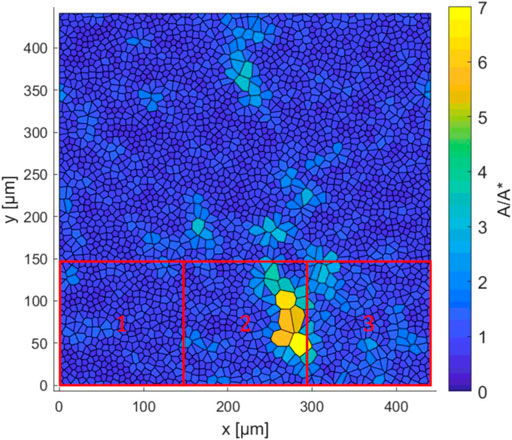
FIGURE 3. Voronoi-polygon areas of the micrograph of Figure 1. Three details are highlighted for visualization of details in following Figures; the size of the details is equal to the SVEs and MVEs generated.

Special attention has to be taken to the periodicity when generating the MVEs. As the goal is to generate fully periodic VEs, all fibers that cut the edge of the VE have to be also present at the opposite edge. Therefore, we copy all fibers intersecting with one of the edges to the opposite edge. This can lead to an intersection of fibers at the edge, which we treat in a second step, where we search for intersecting fibers and decrease their fiber diameter until the intersection is deleted. If the resulting fiber diameter is lower than the threshold value of 5.4 µm, which is the smallest measured diameter, as obtained in separate optical measurements, of the micrographs, the fiber is removed. The algorithm of the MVE generation is schematically visualized in Figure 4.

FIGURE 4

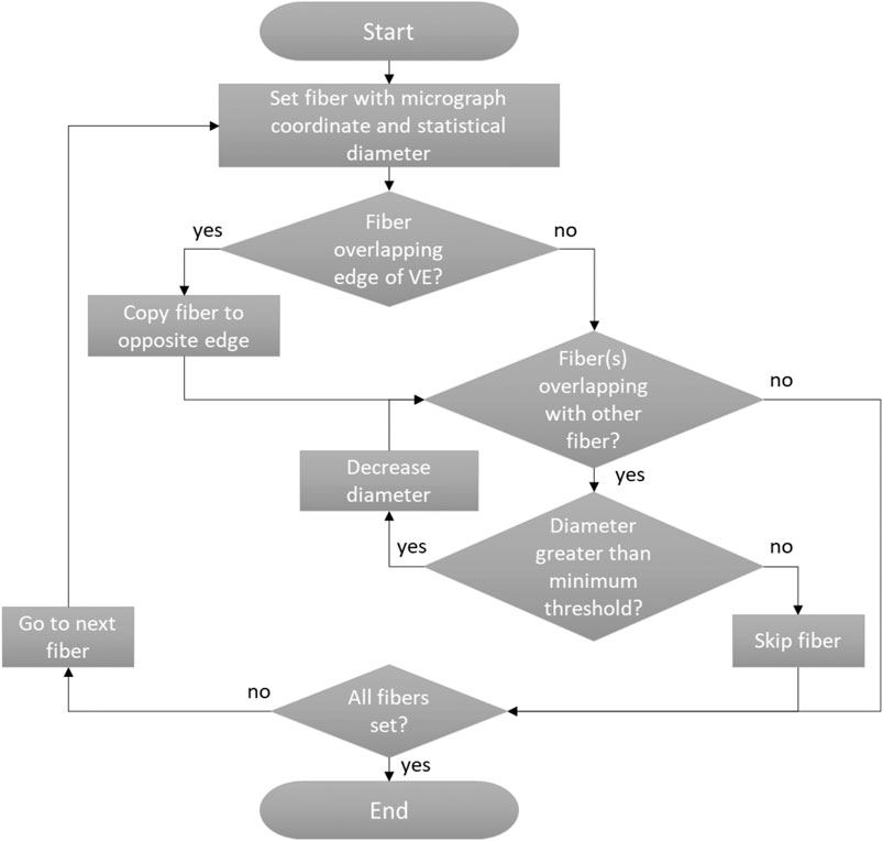
FIGURE 4. MVE generation algorithm using micrograph coordinates and guaranteeing periodicity.

In Figure 5, the Voronoi areas of three example MVE highlighted in Figure 3 are plotted. While Figures 5A,C show a rather homogeneous fiber distribution, Figure 5B contains multiple large polygon areas that correspond to the large pure resin areas that are visible in Figure 3, detail 2. The fiber volume fraction of Figure 5B is 40.7%, compared to values of 53.8 and 42.6% for Figures 5A,C, respectively. The fiber volume fractions of all micrographs vary in a range of 39–59%. Because of the normalization with the fiber volume fraction the normalized area sizes differ slightly compared to Figure 3. The standard deviations of the Voronoi-polygon areas are 0.245, 0.592 and 0.345. The large heterogeneity of Figure 5B is therefore well represented in the much higher standard deviation.

FIGURE 5

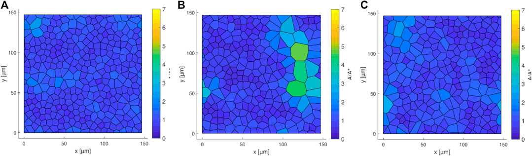
FIGURE 5. Voronoi polygon areas of three MVEs of Figure 1; Larger inter-fiber gaps lead to larger Voronoi-polygon areas; (A) detail 1; (B) detail 2; (C) detail 3.

Additionally to the generation of MVEs, a statistical approach is used where SVEs are generated using the algorithm of Melro et al. (2008). The algorithm contains three main steps. In the first step, the fibers are set randomly inside the VE. In the second and third step, the fibers inside the VE and in the outskirts are stirred and new fibers are inserted as long as the required fiber volume fraction is not reached. By this approach, a random VE with periodic edges for high fiber volume fractions can be generated. The fiber volume fraction $\text{Φ}$ of the SVEs is increased in steps of 5% from 35 to 60%. Matsumura and Jackson (2014) used also periodic boundaries for their micro-scale simulations and reported that at least 10 representative volume elements with 200 fibers should be generated. In our case, we generate 10 SVEs for each configuration set up, which leads to 10 cases in the axial direction and 20 cases in the transverse direction (both horizontal and vertical flow direction are used). The number of fibers varies depending on the fiber volume fraction between 198 and 354. The minimum gap $D_{\text{min}}$ between two fibers is set to 1% of the fiber diameter. This ensures a successful meshing but also leads to a nearly blocking of flow paths for transverse flow, which is important to predict permeability, especially at high fiber volume fraction. The configuration parameters are shown in Table 1.

TABLE 1

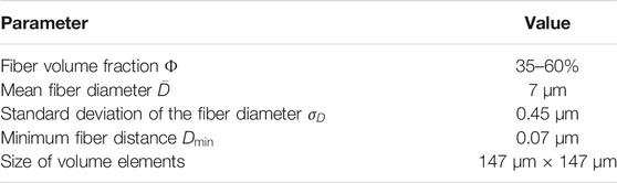
TABLE 1. Configuration parameters of the SVEs; for each configuration, 10 SVEs are generated.

Figure 6 shows the fiber diameter distribution in the MVE highlighted in Figure 5B compared to one exemplary SVE with a fiber volume fraction of 40%. Both graphs show a Gaussian distribution around the mean value of 7 μm, whereas the MVE distribution has a slight deviation of fiber diameters towards smaller values, which is explained by the algorithm used to ensure periodicity.

FIGURE 6

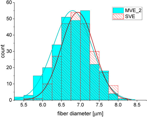
FIGURE 6. Fiber diameter distribution of MVE of Figure 3B compared to an SVE with 40% fiber volume fraction.

In Figure 7, an SVE with a fiber volume fraction of 40% and its resulting Voronoi polygons are visualized. While in Figure 7A the fiber arrangement and the non-constant fiber diameters can be observed, Figure 7B shows a rather homogeneous distribution of the Voronoi polygon areas compared to the MVEs shown in Figure 5. This is also visible, when comparing the standard deviations of the Voronoi-polygon areas ${\sigma }_V$, which are visualized in Figure 8. The standard deviations of the MVEs lie in a range from 0.178 to 0.855, whereas for the SVEs, ${\sigma }_V$ lie between 0.138 and 0.232. For all configurations, a decreasing of the deviations with increasing fiber volume fraction is observed. For the SVEs, this behavior is a result of the increasing difficulty to generate a heterogeneous fiber distribution for higher fiber volume fractions. Large inter-fiber gaps in the MVE lead to a larger ${\mathit{\sigma }}_V$ in general. They also lead to lower fiber volume fractions of these MVEs, which explains the increase of ${\sigma }_V$ for these configurations. It is visible, that the MVEs in general have a higher heterogeneity compared to the SVEs.

FIGURE 7

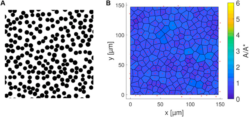
FIGURE 7. Example of an SVE with 40% fiber volume fraction; (A) fiber distribution; (B) Voronoi polygon areas.

FIGURE 8

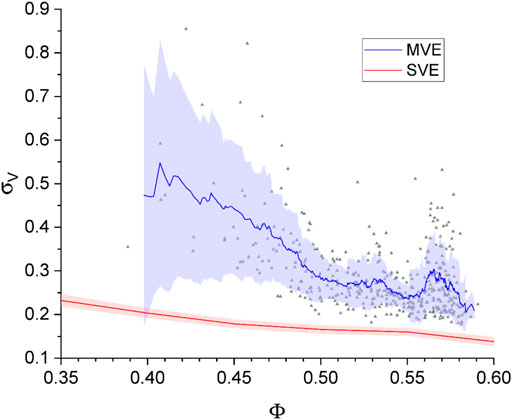
FIGURE 8. Standard deviation of Voronoi-polygon areas ${\mathrm{\sigma }}_{\mathrm{V}}$ of MVEs and SVEs. Grey dots show the individual MVE cases. The highlighted areas show the standard deviation of the moving average of 30 cases for the MVEs and the standard deviation of the 10 SVEs per fiber volume fraction generated.

Numerical Simulations on Micro-Scale

Simulation Model

When simulating volume elements on a micro-scale, it is important to correctly set the boundaries with the aim to minimize their influence on the solution. By using periodic boundaries on all relevant edges, the flow is not restricted to be purely inside the domain, but instead, the fluid is allowed to flow out of and into the domain at the same time. This prevents an influence of the boundary condition onto the solution.

Figure 9 and Figure 10 show an exemplary simulation model with the boundaries and the solution of an axial and a transverse case, respectively. In the axial case, periodic boundaries are used on all faces of the simulation model. Most important are these conditions along the fiber direction and, thus, in the flow direction, which leads to a flow along the continuous filaments. The periodic boundaries at the left/right and top/bottom face pairs are necessary to model the transverse flow. This can be interpreted as a continuous repetition of the volume elements on these sides. The Figures show furthermore the flow velocities resulting at convergence. The different flow paths are visible for the transverse flow in Figure 10, whereas in the axial case, the flow velocity depends on the gap size between the fibers.

FIGURE 9

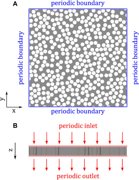
FIGURE 9. Simulation model with periodic boundaries for axial simulations; view parallel (A) and transverse (B) to the fibers.

FIGURE 10

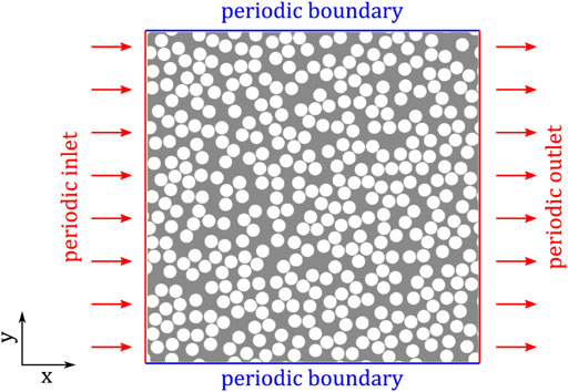
FIGURE 10. Simulation model with periodic boundaries for transverse simulations in x direction; view parallel to the fibers; fiber parallel direction is omitted in the simulations.

Numerical Method

The simulations are performed with a laminar steady state solver that uses a finite volume discretization and the SIMPLE-algorithm implemented in the open-source library OpenFOAM^®. This method is used widely for problems of heat transfer or fluid dynamics. A detailed description of the numerical algorithm can be found in the user guide (CFD Direct 2021) or for example in Ferziger and Perić (2002). The periodic boundaries prohibit applying a pressure or velocity at the boundaries to start the desired laminar flow. Instead, the flow is induced by adding a momentum source to the Navier-Stokes equations by applying a pressure gradient, so that a predefined volume-averaged velocity is obtained (“meanVelocityForce”).

As the permeability is a measure related to the porous drag acting on the fluid, it can be determined by rearranging the one-dimensional Darcy equation to:

$\mathit{K}=-\frac{\mu \cdot \overline{\mathit{U}}\left(1-\text{Φ}\right)}{\text{Δ}p} ,$

with the volume averaged fluid velocity $\overline{\mathit{U}}$ of the porous domain and the pressure gradient $\text{Δ}p$. Three cases are simulated for each VE. Two simulations in x and y direction for flow transverse to the fiber direction and one simulation in z direction for flow parallel to the fiber direction. Therefore, the velocity $\overline{\mathit{U}}$ is set to a target value that contains only one entry in the corresponding flow direction.

This leads to double the number of cases simulated for flow transverse to the fiber direction compared to flow parallel to the fiber direction. In each of the SIMPLE iterations, an incremental additional pressure gradient is calculated based on the volume averaged velocity $\left|\tilde{\mathit{U}}\right|$:

$\left|\tilde{\mathit{U}}\right|=\frac{{{\displaystyle \sum }}_i\left(\frac{\overline{\mathit{U}}}{\left|\overline{\mathit{U}}\right|}\cdot {\mathit{U}}_i\right)\cdot V_i}{{{\displaystyle \sum }}_i{V}_i},$

$d\text{Δ}p=(\left|\overline{\mathit{U}}\right|-|\tilde{\mathit{U}}\left|\right)\cdot \widetilde{a_p},$

with the volume averaged diagonal coefficients of the momentum equation $\widetilde{a_p}$. For details of the discretization procedure used in OpenFOAM, the reader is referred to the work of Jasak (1996). With this pressure gradient, the velocity in each cell i is adjusted to achieve the desired average velocity $\overline{\mathit{U}}$:

${\mathit{U}}_{i,u}={\mathit{U}}_i+\frac{\overline{\mathit{U}}}{\left|\overline{\mathit{U}}\right|}\cdot \frac{1}{a_p}\cdot d\text{Δ}p,$

and the pressure gradient is also updated:

$\text{Δ}{p}_u=\text{Δ}p+d\text{Δ}p$

At convergence, the incremental pressure gradient decreases to zero.

Mesh Study

An important aspect of the simulation model is the mesh cell size. The simulations’ aim is to measure the drag inside the porous medium that is a result of the sum of the shear forces at the surfaces of the fibers. To correctly model these shear forces and, following, the permeability, the cell size has to be small enough to capture the velocity gradient at these fluid filament interfaces. Because of this, a mesh study was performed to find the largest cell sizes that correctly model the flow, but also allow for a reasonable short simulation time.

To mesh the porous domain between the fibers, first, a triangular mesh is generated that can capture the complex geometry of the fiber distribution. For the axial flow cases, this mesh is extruded in fiber direction in a following step. Figure 11 shows a zoomed view of the mesh around the fibers.

FIGURE 11

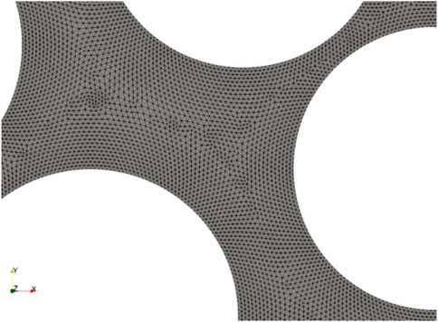
FIGURE 11. Detailed view of the simulation mesh around fibers.

The periodic boundary conditions need an equal cell size (cell edge length) at opposite mesh boundaries. When a meshing algorithm with refinement at the fiber interfaces is used, this cannot be guaranteed. Because of this reason, we use a homogeneous cell size in the simulation domain. To find the necessary maximum cell size and the minimum SIMPLE-iterations needed for convergence, two models with a fiber volume fraction of 20 and 45% with varying cell sizes are simulated.

Figure 12 shows the results of the normalized error that is calculated with the permeability value for the smallest cell size (and maximum iterations) as the nominal value. For each of the configurations, the number of necessary iterations increases with decreasing cell sizes. Smaller cells are needed for higher fiber volume fractions, which was also reported in the literature (Matsumura and Jackson, 2014). The error in the transverse cases is in general higher than in the axial cases. Based on the results of the mesh study, the cell size and iteration number are chosen depending on the fiber volume fraction with the aim to have an error of less than 1%. The used mesh sizes are summarized in Table 2.

FIGURE 12

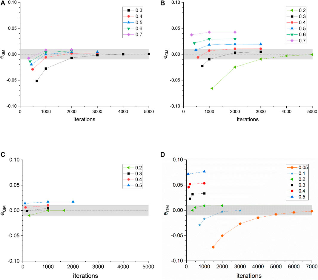
FIGURE 12. Geometric mean permeability error depending on mesh cell size and SIMPLE iterations; (A) axial case with 20% fiber volume fraction; (B) transverse case with 20% fiber volume fraction; (C) axial case with 45% fiber volume fraction; (D) transverse case with 45% fiber volume fraction.

TABLE 2

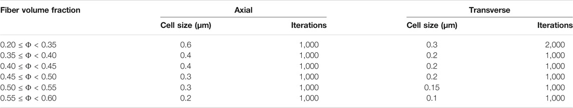
TABLE 2. Simple iteration number and mesh cell size used for simulations.

The simulation times vary strongly depending on the mesh size. The average simulation times for simulations are summarized in Table 3. Simulations were carried out without parallelization on a system with one AMD EPYC 7302P 16-core processor (3.0 GHz) and 256 GB RAM (3,200 MHz). The parallelization strongly decreases the simulation time for all mesh cell sizes.

TABLE 3

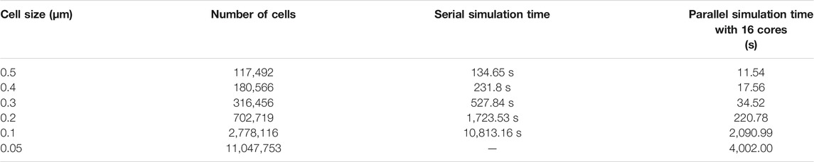
TABLE 3. Simulation times for 1,000 iterations of the transverse case with 45% fiber volume fraction at different cell sizes.

Results

In Figure 13, the results of the flow simulations for the MVEs highlighted in Figure 3 are visualized. The subfigures (A–C) show the results of the flow simulation parallel to the fibers, whereas subfigures (D–F) show the resulting transverse flow (here from left to right). For the axial flow, the highest flow velocity is observed in the large gaps between the fibers. On the contrary, for the transverse flow the highest fluid velocity is observed in the largest channels between the fibers that are connected through the simulation domain. Furthermore, the effect of the periodic boundaries is visible in Figure 13E. Here, one resin channel forms that flows over the top and bottom edge, which would not be possible when using wall type boundary conditions. For both simulation types, large areas of the simulation model show only very low fluid velocities.

FIGURE 13

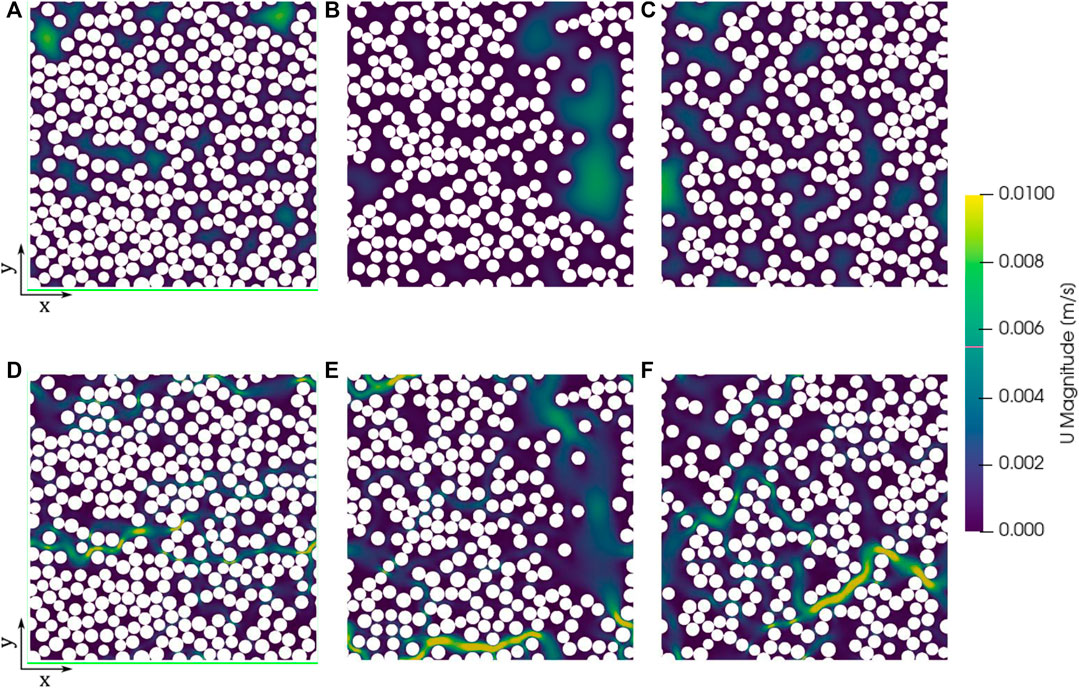
FIGURE 13. Resin flow velocity of the three MVEs of Figure 2 with axial flow: (A) values corresponding to detail 1, (B) values corresponding to detail 2 and (C) values corresponding to detail 3; and the resin flow velocity with transverse flow in x-direction: (D) values corresponding to detail 1, (E) values corresponding to detail 2 and (F) values corresponding to detail 3.

In total, more than 400 MVE configurations are simulated. To compare the SVE model to the MVE simulation results, the resulting permeability values obtained for both, axial and transverse flow, are plotted in Figure 14. The grey crosses and lines show the individual results of the MVE simulations. The permeabilities of the transverse cases in x-direction and y-direction are differentiated by grey horizontal and vertical lines, respectively. No systematic difference of the transverse permeabilities in x-direction and y-direction is observed. Therefore, both transverse permeabilities are merged in the following analyses. The SVE simulation results are shown in red color. For each fiber volume fraction, the average permeability and the standard deviation of 10/20 individual simulations for parallel/transverse flow are calculated. The blue lines are the moving average of 30 individual results of the MVE simulations. The light blue and red areas show the standard deviation of these averages. For the whole range of fiber volume fraction, the axial permeability of the SVE is lower than that of the MVE. In contrast, the transverse permeability of the SVE is higher than the one predicted using MVEs. The permeability predicted by Gebart’s model for hexagonal fiber arrays (Gebart, 1992) is shown in black color. For the axial flow case, it is nearly equal to the SVE simulations and only differs slightly at higher fiber volume fraction. In the transverse case, Gebart’s prediction is higher than the SVE and MVE results over the whole range with increasing difference for large fiber volume fractions, which was also observed by Gommer et al. (2018).

FIGURE 14

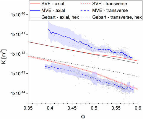
FIGURE 14. Permeability comparison of SVEs, MVEs and Gebart’s equation for hexagonal fiber arrays (Gebart, 1992) for axial and transverse flow. The highlighted areas show the standard deviation of the moving average of 30 cases for the MVEs and the standard deviation of the 10/20 SVEs per fiber volume fraction generated. The grey crosses and lines mark the individual simulation results.

In the transverse permeability of the MVEs, some outliers are visible at around 50% fiber volume fraction. The flow velocities of one of those is visualized in Figure A1 in the Appendix. Here, a large horizontal gap is present that leads to significantly higher permeability in x-direction than in y-direction.

Furthermore, the normalized difference between the averages of the SVE and MVE simulations is visualized in Figure 15. This error value is calculated with a normalization using the geometric mean of the values:

$e_{\text{GM}}=\frac{K_{\text{MVE}}-K_{\text{SVE}}}{\sqrt{K_{\text{MVE}}\cdot K_{\text{SVE}}}} .$

FIGURE 15

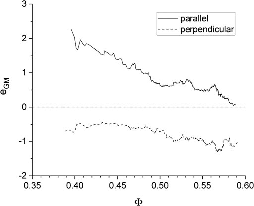
FIGURE 15. Normalized difference between SVE and MVE permeability.

The difference of the axial permeability decreases with increasing fiber volume fraction, whereas the error of the transverse flow increases slightly at negative values.

Discussion

The analyses of the micrograph images reveal a heterogeneous fiber distribution inside the analyzed rovings. This confirms the observations made by Gommer et al. (2016), though a different type of material was used, which indicates the independence of the heterogeneity of the micro-scale fiber distribution of the material type. However, for a detailed analysis, further investigations of micrographs are necessary.

When using a random VE generator, the heterogeneity of the fiber distribution is much lower than in real micrographs, which can directly be deduced from the variance of the Voronoi-polygon areas plotted in Figure 8. For higher fiber volume fraction, the variance of the Voronoi-polygon areas is lower, which indicates a stricter arrangement of the filaments at higher fiber volume fractions. For low fiber volume fractions, the variance is high, since larger gaps between the fibers exist.

The scatter of the variance is very high especially in the range of 55–60% fiber volume fraction. This is the result of some smaller gaps inside densely packed arrangements that are also visible in Figure 3. The influence of these heterogeneities on the micro-scale permeability is analyzed using periodic VEs and CFD simulations. First of all, the strong influence of the fiber volume fraction and fiber orientation (axial vs transverse) onto the permeability is obvious. Furthermore, the permeabilities in Figure 14 and their normalized differences in Figure 15 show that the results of the SVE differ from the MVE results significantly. While the axial permeability of the MVEs is higher than that of the SVEs with a maximum value of over 2, the transverse permeability shows the opposite with a minimum normalized difference lower than −1. When comparing the results for a given fiber volume fraction, this leads to the conclusion that a stronger heterogeneity leads to higher permeability in axial flow and to lower permeability in transverse flow. This is explained by the fact that for axial flow, the permeability significantly depends on the flow inside large gaps, whereas the flow between very close fibers can be neglected. For a transverse flow instead, the permeability depends on the size and number of flow channels that are formed between the fibers. Here, larger gaps may lead to flow channels but on the contrary, they also lead to more densely packed fibers in other areas (at constant fiber volume fraction). In Figure 16, the standard deviation ${\sigma }_{\text{V}}$ of the Voronoi-polygon areas and the normalized differences of the permeabilities of MVEs and SVEs are visualized to allow a direct comparison. It is visible that the course of the standard deviation curve follows a similar local and overall trend compared to the curve showing the parallel flow cases. The curve of the transverse case does not show this clear trend.

FIGURE 16

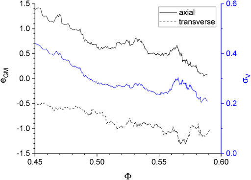
FIGURE 16. Standard deviation of the Voronoi polygon areas ${\mathrm{\sigma }}_{\mathrm{V}}$ and normalized errors of axial and transverse flow.

To analyze the correlation between the permeability $K$ and the fiber volume fraction as well as the standard deviation of the Voronoi polygon areas, the Pearson correlation coefficient is used:

$c{c}_{\text{P}}=\frac{cov\left(K,\text{Ψ}\right)}{{\sigma }_K\cdot {\sigma }_{\text{Ψ}}} ,$

where $\text{Ψ}$ is one of the analyzed parameters and with cov(.) meaning the covariance. The Pearson correlation coefficients are shown in Figure 17. It is applied on $\text{log}\left(K\right)$ to linearize the values, which is a requirement for a correct interpretation of the correlation coefficient. The coefficient is zero when no correlation is present and -1 or +1 for a perfect negative or positive correlation, respectively. A higher fiber volume fraction leads to lower permeability, which is visualized by the coefficients that show a strong negative correlation between $\text{log}\left(K\right)$ and fiber volume fraction. The graph also shows a positive correlation to ${\sigma }_{\text{V}}$ for both cases, which means that a higher fiber heterogeneity (quantified by ${\sigma }_{\text{V}}$) leads to a higher permeability. The correlation of ${\sigma }_{\text{V}}$ to $\text{log}\left(K\right)$ is stronger in the axial cases (0.650) than in the transverse cases (0.495), which confirms the observations of Figure 16. When calculating the Pearson correlation coefficients only for the cases of transverse flow in x-direction or in y direction, the values differ only slightly (0.484 compared to 0.503). Thus, the flow direction in the transverse cases does not play a major role.

FIGURE 17

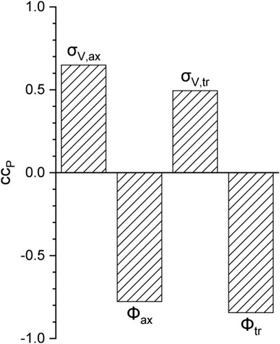
FIGURE 17. Pearson correlation coefficient for ${\mathrm{\sigma }}_{\mathrm{V}}$ and fiber volume fraction.

Conclusion

In the present work, micrograph images of the cross-sections of manufactured samples were taken to analyze the micro-scale fiber arrangement. The carbon fibers inside the rovings show a heterogeneous distribution containing densely packed areas and also larger gaps between fibers. The distribution was analyzed by generating Voronoi-polygons between the fiber center points. It is shown that the deviation of these Voronoi-polygon areas is higher in the micrographs than in a generated statistical distribution. To analyze this influence on the micro-scale permeability, periodic VEs are generated for the micrographs (MVE) and for the statistical approach (SVE). By simulating a stationary fluid flow between the fibers, the permeability is computed numerically. The results show that the different fiber distribution directly influences the permeability transverse and axial to the fiber direction. In the axial case the MVE permeability is higher than the SVE permeability. On contrary, in the transverse case, the MVE permeability is lower than the SVE permeability.

The correlation analysis shows the dependency of the permeability on fiber volume fraction and Voronoi-polygon area variance. The latter is therefore a useful parameter to describe the heterogeneity of the fiber distribution, especially when large resin-rich areas are present, which is not guaranteed when using nearest neighbor descriptors. Therefore, the Voronoi-polygon area variance is proposed to be included in future micro models, especially for predicting fiber parallel permeability.

The work shows that methods to generate statistical models with higher heterogeneity of the fiber microstructure are necessary to realistically predict the micro-scale permeability. Resin-rich areas also influence the micro-mechanical behavior, which was recently investigated by Ghayoor et al. (2019). This further depicts the necessity of improved methods to generate statistical micro-models.

In the method presented here, the fibers are assumed to be straight and perfectly parallel. In future work, it should be analyzed, how curved or twisted fibers change the pore network and how this influences the three-dimensional permeability of TFP rovings. Additionally, by using high-resolution computer tomography or micrographs, the fiber diameter distribution and the cross-section geometries can be measured to analyze their influence on the permeability prediction.

Furthermore, it is still important to validate the permeability predictions with experiments. Therefore, in the next work, a meso-scale model for TFP infiltration under RTM process conditions is developed to take the inter-roving flow into consideration. The permeability of the meso-scale models can afterwards be compared to infiltration experiments with stitched TFP preforms. This finally enables the prediction of the mold-filling pattern and filling time of composite parts made by TFP.

Data Availability Statement

The original contributions presented in the study are included in the article/supplementary material, further inquiries can be directed to the corresponding author.

Author Contributions

Conceptualization: JS; Methodology: LB, JS and LC; Micrographs: LB; Simulations: LC and JS; Writing—original draft preparation: JS, LB and LC; Writing—review and editing: AS and LK; Visualization: JS, LB and LC; Supervision: AS and LK.

Funding

This work is funded by the Deutsche Forschungsgemeinschaft (DFG, German Research Foundation), project KA 4224/4-1 and SP 1646/2-1 “Methods and process development for the infiltration of highly loadable topology-optimized fiber-reinforced composites with a variable-axial fiber architecture (MerVa),” grant no. 415041798. The work is also part of the Young Investigator Group (YIG) “Green Mobility,” generously funded by the Vector Stiftung.

Conflict of Interest

The authors declare that the research was conducted in the absence of any commercial or financial relationships that could be construed as a potential conflict of interest.

Publisher’s Note

All claims expressed in this article are solely those of the authors and do not necessarily represent those of their affiliated organizations, or those of the publisher, the editors and the reviewers. Any product that may be evaluated in this article, or claim that may be made by its manufacturer, is not guaranteed or endorsed by the publisher.

References

Arbter, R., Beraud, J. M., Binetruy, C., Bizet, L., Bréard, J., Comas-Cardona, S., et al. (2011). Experimental Determination of the Permeability of Textiles: A Benchmark Exercise. Compos. A: Appl. Sci. Manuf. 42 (9), 1157–1168. doi:10.1016/j.compositesa.2011.04.021

CrossRef Full Text | Google Scholar

Åström, B. T., Pipes, R. B., and Advani, S. G. (1992). On Flow through Aligned Fiber Beds and its Application to Composites Processing. J. Compos. Mater. 26 (9), 1351–1373. doi:10.1177/002199839202600907

CrossRef Full Text | Google Scholar

Bechtold, G., and Ye, L. (2003). Influence of Fibre Distribution on the Transverse Flow Permeability in Fibre Bundles. Compos. Sci. Tech. 63 (14), 2069–2079. doi:10.1016/S0266-3538(03)00112-X

CrossRef Full Text | Google Scholar

Bittrich, L., Spickenheuer, A., AlmeidaJosé Humberto, J. H. S., Müller, S., Kroll, L., and Heinrich, G. (2019). Optimizing Variable-Axial Fiber-Reinforced Composite Laminates: The Direct Fiber Path Optimization Concept. Math. Probl. Eng. 2019 (3), 1–11. doi:10.1155/2019/8260563

CrossRef Full Text | Google Scholar

Bradski, G. (2000). The OpenCV Library. Dr. Dobb’s Journal of Software Tools.

Google Scholar

Cai, Z., and Berdichevsky, A. L. (1993). Numerical Simulation on the Permeability Variations of a Fiber Assembly. Polym. Compos. 14 (6), 529–539. doi:10.1002/pc.750140611

CrossRef Full Text | Google Scholar

Carman, P. C. (1937). “Fluid Flow through Granular Beds,” in Trans. INSTN Chemical Engineers CFD Direct (2021): OpenFOAM User Guide. Available at: https://cfd.direct/openfoam/user-guide/.

Google Scholar

Chen, X., and Papathanasiou, T. D. (2008). The Transverse Permeability of Disordered Fiber Arrays: a Statistical Correlation in Terms of the Mean Nearest Interfiber Spacing. Transp Porous Med. 71 (2), 233–251. doi:10.1007/s11242-007-9123-6

CrossRef Full Text | Google Scholar

Chen, X., and Papathanasiou, T. (2007). Micro-scale Modeling of Axial Flow through Unidirectional Disordered Fiber Arrays. Composites Sci. Tech. 67 (7-8), 1286–1293. doi:10.1016/j.compscitech.2006.10.011

CrossRef Full Text | Google Scholar

Darcy, H. (1856). Les Fontaines publiques de la ville de Dijon. Paris: Dalmont.

Google Scholar

Endruweit, A., Gommer, F., and Long, A. C. (2013). Stochastic Analysis of Fibre Volume Fraction and Permeability in Fibre Bundles with Random Filament Arrangement. Compos. Part A: Appl. Sci. Manuf. 49, 109–118. doi:10.1016/j.compositesa.2013.02.012

CrossRef Full Text | Google Scholar

Ferziger, J. H., and Perić, M. (2002). Computational Methods for Fluid Dynamics. Berlin, Heidelberg: Springer Berlin Heidelberg. doi:10.1007/978-3-642-56026-2

CrossRef Full Text | Google Scholar

Gebart, B. R. (1992). Permeability of Unidirectional Reinforcements for RTM. J. Compos. Mater. (26), 1100–1133. doi:10.1177/002199839202600802

CrossRef Full Text | Google Scholar

Ghayoor, H., Marsden, C. C., Hoa, S. V., and Melro, A. R. (2019). Numerical Analysis of Resin-Rich Areas and Their Effects on Failure Initiation of Composites. Compos. Part A: Appl. Sci. Manuf. 117 (5), 125–133. doi:10.1016/j.compositesa.2018.11.016

CrossRef Full Text | Google Scholar

Gommer, F., Endruweit, A., and Long, A. C. (2018). Influence of the Micro-structure on Saturated Transverse Flow in Fibre Arrays. J. Compos. Mater. 52 (18), 2463–2475. doi:10.1177/0021998317747954

CrossRef Full Text | Google Scholar

Gommer, F., Endruweit, A., and Long, A. C. (2016). Quantification of Micro-scale Variability in Fibre Bundles. Compos. Part A: Appl. Sci. Manuf. 87, 131–137. doi:10.1016/j.compositesa.2016.04.019

CrossRef Full Text | Google Scholar

Henning, F., Kärger, L., Dörr, D., Schirmaier, F. J., Seuffert, J., and Bernath, A. (2019). Fast Processing and Continuous Simulation of Automotive Structural Composite Components. Compos. Sci. Tech. 171, 261–279. doi:10.1016/j.compscitech.2018.12.007

CrossRef Full Text | Google Scholar

Jasak, H. (1996). Error Analysis and Estimation for the Finite Volume Method with Applications to Fluid Flows. LondonTechnology and Medicine: University of LondonImperial College of Science.

Google Scholar

Kärger, L., Bernath, A., Fritz, F., Galkin, S., Magagnato, D., Oeckerath, A., et al. (2015). Development and Validation of a CAE Chain for Unidirectional Fibre Reinforced Composite Components. Compos. Struct. 132, 350–358. doi:10.1016/j.compstruct.2015.05.047

CrossRef Full Text | Google Scholar

Kozeny, J. (1927). Ueber kapillare Leitung des Wassers im Boden. Sitzungsber. Akad. Wiss. 136 (2a), 271–306.

Google Scholar

Magagnato, D., and Henning, F. (2015). Process-Oriented Determination of Preform Permeability and Matrix Viscosity During Mold Filling in Resin Transfer Molding. Mater. Sci. Forum 825–826, 822–829. doi:10.4028/www.scientific.net/MSF.825-826.822

PubMed Abstract | CrossRef Full Text | Google Scholar

Matsumura, Y., and Jackson, T. L. (2014). Numerical Simulation of Fluid Flow through Random Packs of Cylinders Using Immersed Boundary Method. Phys. Fluids 26 (4), 043602. doi:10.1063/1.4870246

CrossRef Full Text | Google Scholar

Mattheij, P., Gliesche, K., and Feltin, D. (1998). Tailored Fiber Placement-Mechanical Properties and Applications. J. Reinforced Plastics Compos. 17 (9), 774–786. doi:10.1177/073168449801700901

CrossRef Full Text | Google Scholar

May, D., Aktas, A., Advani, S. G., Berg, D. C., Endruweit, A., Fauster, E., et al. (2019). In-plane Permeability Characterization of Engineering Textiles Based on Radial Flow Experiments: A Benchmark Exercise. Compos. Part A: Appl. Sci. Manuf. 121, 100–114. doi:10.1016/j.compositesa.2019.03.006

CrossRef Full Text | Google Scholar

Melro, A., Camanho, P., and Pinho, S. (2008). Generation of Random Distribution of Fibres in Long-Fibre Reinforced Composites. Compos. Sci. Tech. 68 (9), 2092–2102. doi:10.1016/j.compscitech.2008.03.013

CrossRef Full Text | Google Scholar

Poppe, C. T., Krauß, C., Albrecht, F., and Kärger, L. (2021). A 3D Process Simulation Model for Wet Compression Moulding. Compos. Part A: Appl. Sci. Manuf. 145 (17), 106379. doi:10.1016/j.compositesa.2021.106379

CrossRef Full Text | Google Scholar

Rimmel, O., and May, D. (2020). Modeling Transverse Micro Flow in Dry Fiber Placement Preforms. J. Compos. Mater. 54 (13), 1691–1703. doi:10.1177/0021998319884612

CrossRef Full Text | Google Scholar

Seuffert, J., Rosenberg, P., Kärger, L., Henning, F., Kothmann, M. H., and Deinzer, G. (2020). Experimental and Numerical Investigations of Pressure-Controlled Resin Transfer Molding (PC-RTM). Adv. Manuf.: Polym. Compos. Sci. 6 (3), 154–163. doi:10.1080/20550340.2020.1805689

CrossRef Full Text | Google Scholar

Spickenheuer, A., Schulz, M., Gliesche, K., and Heinrich, G. (2008). Using Tailored Fibre Placement Technology for Stress Adapted Design of Composite Structures. Plast. Rubber Compos. 37 (5), 227–232. doi:10.1179/174328908X309448

CrossRef Full Text | Google Scholar

Um, M. K., and Lee, W. I. (1997). A Study on Permeability of Unidirectional Fiber Beds. J. Reinf. Plast. Compos. 16, 1575–1590. doi:10.1177/073168449701601704

CrossRef Full Text | Google Scholar

Vernet, N., Ruiz, E., Advani, S., Alms, J. B., Aubert, M., Barburski, M., et al. (2014). Experimental Determination of the Permeability of Engineering Textiles: Benchmark II. Compos. Part A: Appl. Sci. Manuf. 61, 172–184. doi:10.1016/j.compositesa.2014.02.010

CrossRef Full Text | Google Scholar

Yazdchi, K., and Luding, S. (2013). Upscaling and Microstructural Analysis of the Flow-Structure Relation Perpendicular to Random, Parallel Fiber Arrays. Chem. Eng. Sci. 98, 173–185. doi:10.1016/j.ces.2013.04.049

CrossRef Full Text | Google Scholar

Yazdchi, K., Srivastava, S., and Luding, S. (2012). Micro-macro Relations for Flow through Random Arrays of Cylinders. Compos. Part A: Appl. Sci. Manuf. 43 (11), 2007–2020. doi:10.1016/j.compositesa.2012.07.020

CrossRef Full Text | Google Scholar

Yong, A. X. H., Aktas, A., May, D., Endruweit, A., Advani, S., Hubert, P., et al. (2021). Out-of-Plane Permeability Measurement for Reinforcement Textiles: A Benchmark Exercise. Compos. Part A: Appl. Sci. Manuf. 148, 106480. doi:10.1016/j.compositesa.2021.106480

CrossRef Full Text | Google Scholar

Zarandi, M. A. F., Arroyo, S., and Pillai, K. M. (2019). Longitudinal and Transverse Flows in Fiber Tows: Evaluation of Theoretical Permeability Models through Numerical Predictions and Experimental Measurements. Compos. Part A: Appl. Sci. Manuf. 119 (6), 73–87. doi:10.1016/j.compositesa.2018.12.032

CrossRef Full Text | Google Scholar

Appendix

FIGURE A1

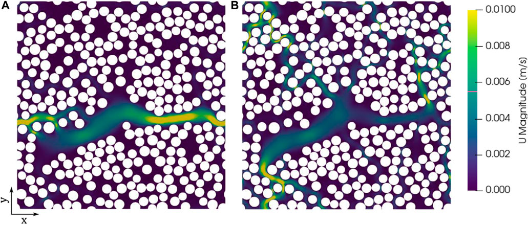
FIGURE A1. Flow velocity results in (A) x-direction and (B) y-direction of one outlier with 50.06% fiber volume fraction. The resulting transverse permeabilities in x-direction and y-direction are $2.47629\cdot {10}^{-13}$ and $3.09254\cdot {10}^{-14}$, respectively.