Static and Kinetic Friction From Nanoscale Slip—A Multiscale Approach Using a 2D Binary Hierarchy of Nodes

A local, elastic deformation model is combined with a dynamic simulation to investigate nanoscale slip between a rigid, curved pin and an elastic slab, and its influence on static and kinetic friction. The elastic deformation model utilizes a novel multiscale grid based on a binary hierarchy. To maximize accuracy, bi-quadratic functions are introduced to interpolate the stresses on the boundaries of the nodal elements. The onset of slip is based on a maximum allowable nodal shear stress to nodal pressure ratio. A nanoscale friction function is developed by translating the pin quasistatically across the slab. The effect of the nanoscale friction profile on a dynamic system is investigated by integrating the equations of motions governing the pin as it is pulled by a stage via a coupling spring. A direct connection is found between the nanoscale slip characteristics and macroscopically observed static and kinetic coefficients of friction.

1 Introduction

Friction has been investigated for many years and early published work on the subject includes that of Amontons (Amontons, 1699), and Coulomb (Coulomb, 1785). Amontons was probably the first to formally state the laws of friction (for dry contact). The first of these states that the friction force is proportional to the normal load, while the second asserts that the friction force is independent of the apparent area of contact. Despite these relationships being referred to as “laws”, it is recognized that they are only approximately held. Nevertheless, it is found for a given material pair, that the ratio of friction force to normal load remains nearly constant over a wide range of load, apparent contact area and sliding speed, leading to the concept of assigning a coefficient of friction (COF) to an interface of given material type. Another important experimental observation is that the friction force required to initiate sliding is almost always greater than that required to sustain sliding. Therefore, one can readily identify two distinct friction coefficients: 1) a static COF, µ_s, defined as the ratio of friction force to normal load at the threshold of sliding and 2) a kinetic COF, µ_k, defined as the ratio of friction force to normal load during the sliding process. The existence of two friction coefficients gives rise to the well-known phenomenon of stick-slip motion in mechanical systems with sufficient compliance, whereby the interface cycles between modes of sticking and slipping. Stick-slip behavior can be detrimental to the operation of machines by inducing undesirable vibration and/or noise (Stewart and Hunt, 1970; Kato et al., 1974; Ioannidis et al., 2002). On the other hand, stick-slip motion may be harnessed to generate desired sounds as done, for example, by certain insects for communication (Haskell, 1961; Patek, 2001), and by violinists in playing music (Helmholtz and Ellis, 1954; Smith and Woodhouse, 2000).

From a macroscopic perspective, sliding means that the contacting surface of one body has a velocity in the plane of the interface that is different from that of the contacting surface of the opposing body. Moreover, when an idealized rigid block slides without rotation across a stationary table, the surface points of the block have the velocity of the block while the surface points of the table are at rest. This simple picture makes the question of sliding clear cut: If the block is moving, there is sliding; otherwise the opposing surface points have no relative motion and are “stuck” together. Yet, reality is more complex. When a body can deform, its surface points can take on velocities that are different from the overall translational velocity of the body. In this scenario, at any given instant, some interfacial regions may be experiencing stick while others are experiencing slip. Additionally, since nearly all solid surfaces possess greater than atomic scale roughness, the actual contact between bodies occurs on some (typically small) fraction of the apparent or nominal contact area. Thus, the sliding process depends upon the way in which the various contact regions engage and disengage. In this work, we are interested in the interfacial conditions governing the onset of macroscopic sliding as well as the behavior of the interface during the sliding process. Specifically, we wish to demonstrate how interactions at micro and nano scales give rise to macroscopic observations. In doing so we hope to provide insight into the ubiquitous phenomenon of friction.

Over the years, various papers have investigated interfacial slip and its impact upon sliding. One early model that has been widely cited is the Burridge-Knopoff (BK) model (Burridge and Knopoff, 1967), which was developed to better understand the behavior of earthquakes. The BK model involves the dynamic motion of a linear array of blocks, each of which is coupled by a leaf spring to a horizontally translating support, as well as coupled to its two nearest neighbors by linear springs, with each block interacting with a stationary surface via frictional contact. The interaction of each block with the counter surface is governed by a prescribed friction law that includes a maximum static friction force limit as well as a sliding-speed-dependent kinetic friction force. The support is translated at a constant low speed and the equations of motions are numerically integrated to provide time histories of displacement. Initially, all blocks are held stationary via static friction by the fixed counter surface. (Alternatively, and equivalently, the support could be held fixed whilst the counter surface is translated.) For each block, the friction force required to keep it motionless increases with increasing horizontal displacement of the support as the leaf spring that couples it to the moving support increases its deflection. Eventually, the required friction force reaches the block’s static friction limit, causing the block to slip against the counter surface. At the same time, the friction forces experienced by both nearest-neighbor blocks are increased due to their coupling with the slipping block. These enhanced friction forces may induce slip in one or both neighbors, which may, in turn, cause slip in their neighbors, and so on. The totality of slips from the first slip until the re-establishment of the condition whereby no blocks experience a friction force above the static friction limit is considered an “avalanche” or an “earthquake”. Despite its simplicity, this and similar models have enjoyed success in capturing important experimentally-observed phenomena, such as the Gutenberg-Richter law (Gutenberg and Richter, 1955), which relates the energy released in an avalanche of slips to the frequency of occurrence.

The dynamic model of BK, as well as closely-related two-dimensional quasistatic versions (Brown et al., 1991; Olami et al., 1992) have been used in the study of sliding friction (Persson, 1995; Braun and Röder, 2002; Braun and Peyrard, 2008; Braun et al., 2009; Braun, 2010; De Moerlooze et al., 2010; Filippov and Popov, 2010). In the quasistatic approach, the process starts with each block displaced a random amount along the axis of support motion. Each block is assigned a maximum attainable static friction force (which may be drawn randomly from a chosen distribution), which, when exceeded, gives rise to block slip, while are all other blocks are held fixed. Typically, a slipping block is then given a new position corresponding to a (temporary) total loss of friction. The friction forces felt by all adjoining blocks are updated in accordance with changing forces in the associated coupling springs. The resulting friction force at each new block (i.e., that required to keep it stuck) is assessed to see if it exceeds the block’s static friction force limit. If no contacts have exceeded their limits, the step is complete. If, on the other hand, at least one block is found to exceed its force limit, then the “most offending” block is allowed to slip and thereby reposition itself to a place of zero friction force, while all other blocks (including the first slipped block are held fixed). The process continues until a state is reached whereby every block experiences a contact force that is less than its static friction force limit. Then the support is displaced again to initiate the next slip. One advantage of the quasistatic approach is that it avoids the computational effort associated with numerically integrating equations of motion. Moreover, as detailed previously (Avlonitis et al., 2014), it is possible to determine, at the end of each step, the precise support displacement (or countersurface displacement) required to initiate the next slip event.

In addition to the above formulations, there has been some relatively recent work applying mean field theory (MFT) to analyze the statistics of interfacial slip, which has been supported by experimental observations (Dahmen et al., 2017; Zhang et al., 2017; Cao et al., 2018; Zheng et al., 2020). In particular, it has been observed that interfaces covering a wide range of length scale show a similar behavior as it relates to magnitude of energy release and frequency of occurrence.

The current work is motivated by the desire to improve the model of interfacial slip by replacing the typical array of harmonically coupled blocks with a linear-elastic slab; i.e., one that satisfies the equations of elastostatics. Additionally, to achieve horizontal and vertical body dimensions that are orders of magnitude larger than the nodal spacing, the model is comprised of a binary-hierarchy of nodes that get increasingly coarse as one moves vertically away from the interface. To optimize computational accuracy with such a nodal configuration, bi-quadratic interpolating functions are implemented to capture the local character of the displacement fields. This interfacial model is used to simulate the sliding of a rigid curved body (“pin”) across an elastic slab under conditions of controlled displacement, which is used to generate a force-displacement curve. Here a “typical” pin-on-flat contact geometry is considered, whereby the contact width is on the order of microns. As will be shown, the characteristic slip distance for such a contact is on the scale of nanometers, giving rise to rapid fluctuations in the friction force as a function of distance. The force-displacement curve, in turn, is used with a spring-mass-damper system to simulate macroscopic observations of static and kinetic friction.

2 Mathematical Modeling

2.1 Nanoscale Friction Model

2.1.1 General Considerations

Figure 1 shows the interface of interest. A rigid, curved pin indents a linear elastic slab, which is prescribed to deform under plane-strain conditions (i.e., there is uniformity normal to the plane of the figure). A constant load is applied to the bottom surface of the slab, while the pin is translated to the right under conditions of prescribed displacement. Outside of the contact zone, the upper surface of the slab is stress free. A restraint is used to prevent lateral displacement of the slab, which experiences lateral forces from frictional contact with the pin. Aside from the restraint, the sides of the slab are stress free. Within the interface, only non-negative pressures are allowed. Additionally, at any given point, the shear stress is not allowed to exceed a fixed factor (µ_i), which is assumed to be an intrinsic or local coefficient of friction. This assumption is applied for convenience and in the absence of an established fundamental relationship operating at the local level. In general, interactions at the atomic scale are rich and varied (Dong et al., 2013; Streator, 2019), and are determined by the details of the intermolecular potentials within each body and across the interface. Here we implement a condition that is based on a popular approach to modeling local friction for a continuum (Johnson, 1985). Now the deformation of the elastic slab is governed by,

$\left(\lambda +2G\right)\frac{{\partial }^{2}u}{\partial x^2}+G\frac{{\partial }^{2}u}{\partial z^2}+\left(\lambda +G\right)\frac{{\partial }^{2}w}{\partial x\partial z}=0(1)$

$\left(\lambda +2G\right)\frac{{\partial }^{2}w}{\partial z^2}+G\frac{{\partial }^{2}w}{\partial x^2}+\left(\lambda +G\right)\frac{{\partial }^{2}u}{\partial x\partial z}=0(2)$

with the surface stresses given by

$\begin{array}{c}{\text{σ}}_x=\left(\lambda +2G\right)\frac{\partial u}{\partial x}+\lambda \frac{\partial w}{\partial z}\\ {\tau }_{xz}=G\left(\frac{\partial u}{\partial z}+\frac{\partial w}{\partial x}\right)\\ -p={\text{σ}}_z=\left(\lambda +2G\right)\frac{\partial w}{\partial z}+\lambda \frac{\partial u}{\partial x}\end{array}(3)$

where λ is the Lamme constant and G is the shear modulus.

FIGURE 1

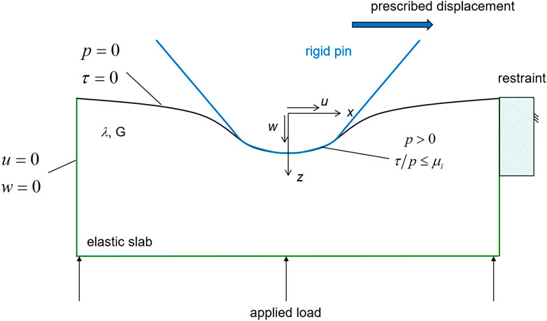
FIGURE 1. Schematic of the interface under investigation.

To initiate a simulation, the equilibrium normal contact configuration is first established. An initial guess is made for the equilibrium interference (the geometric overlap between the pin and the undeformed slab). For the given applied load, the vertical position of the slab along with its contact configuration is iterated through successive static equilibrium configurations and the following interfacial constraints are imposed:

I. All contact pressures are non-negative

II. The ratio of shear stress to pressure within the contact zone does not exceed µ_i.

III. The height of the slab surface never exceeds the height of the pin surface at a given value of the x-coordinate.

Once the normal contact configuration is established, the sliding simulation is initiated by prescribing the minimum lateral displacement to initiate a triggering event, which is defined to be the temporary violation of one of the interfacial constraints listed above. The most common violation is the ratio of shear stress to pressure exceeding the prescribed intrinsic friction coefficient (µ_i). In any case, the contact configuration must be iterated through successive provisional equilibrium configurations until each of the interfacial constraints is satisfied, thereby establishing the equilibrium configuration associated with the given pin displacement. This iteration process often results in multiple instances of slip for each displacement step of the rigid pin. Of particular interest in the current work is the dependence of friction force on lateral pin displacement.

2.1.2 Binary Hierarchy of Nodes

Figure 2 shows an illustration of the binary, hierarchical nodal network used in the present study. Each of the top two nodal layers contains $n_x= 2^N+1$ nodes, where N is an integer. (N = 4 in Figure 2). The remaining rows are populated with $2^{N-1}+1$, $2^{N-2}+1$, $2^{N-3}+1$ nodes, respectively, for the desired number of rows, with three being the minimum possible number of nodes for the bottom row of nodes. For all the simulations in the present work we choose the maximum possible number of rows for the chosen value of $n_x$. The broken lines in Figure 2 indicate the boundaries of the control volumes associated with each node. As detailed in the next section, a force balance is applied to each nodal control volume to develop the equations of equilibrium. The binary structure is designed to optimize the computational accuracy for a given level of computational effort.

FIGURE 2

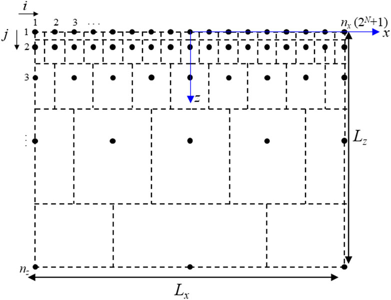
FIGURE 2. Grid structure base on a binary hierarchy. Broken lines show the control volume associate with each node.

2.1.3 Nodal Volume Elements and Interpolating Functions

Consider a representative control volume, as shown in Figure 3, whose corresponding node is in nodal row j and where $\left(x_{ij}, z_j\right)$ denotes the location of the node. Static equilibrium dictates that the net force in both the x- and z-directions (per unit length in the y-direction) must vanish. Assuming that there are no external forces applied to the nodal control volume, it means that the net force exerted upon it due to normal and shear stresses at its four boundaries must equal zero. To establish a force balance on the control volume of Figure 3, we develop an approximation to the force per unit depth acting on each of the control volume boundaries by implementing interpolating functions that describe the local displacement field. For the typical nodal control volume, this formulation can be written as:

$f_x^S=\underset{z_j-\frac{1}{2}\mathrm{\Delta }{z}_j}{\overset{z_j+\mathrm{\Delta }{z}_j}{{\displaystyle \int }}}\left[{{\sigma }_x|}_{x_{ij}+\frac{1}{2}\mathrm{\Delta }{x}_j}-{{\sigma }_x|}_{x_{ij}-\frac{1}{2}\mathrm{\Delta }{x}_j}\right]dz+\underset{x_{ij}-\frac{1}{2}\mathrm{\Delta }{x}_j}{\overset{x_{ij}+\frac{1}{2}\mathrm{\Delta }{x}_j}{{\displaystyle \int }}}\left[{{\tau }_{xz}|}_{z_j+\mathrm{\Delta }{z}_j}-{{\tau }_{xz}|}_{z_j-\frac{1}{2}\mathrm{\Delta }{z}_j}\right]dx(4)$

$f_z^S=\underset{x_{ij}-\frac{1}{2}\mathrm{\Delta }{x}_j}{\overset{x_{ij}+\frac{1}{2}\mathrm{\Delta }{x}_j}{{\displaystyle \int }}}\left[{{\sigma }_z|}_{z_j+\mathrm{\Delta }{z}_j}-{{\sigma }_z|}_{z_j-\frac{1}{2}\mathrm{\Delta }{z}_j}\right]dx+\underset{z_j-\frac{1}{2}\mathrm{\Delta }{z}_j}{\overset{z_j+\mathrm{\Delta }{z}_j}{{\displaystyle \int }}}\left[{{\tau }_{xz}|}_{x_{ij}+\frac{1}{2}\mathrm{\Delta }{x}_j}-{{\tau }_{xz}|}_{x_{ij}-\frac{1}{2}\mathrm{\Delta }{x}_j}\right]dz(5)$

where $f_x^S$ and $f_z^S$ denote the net “spring” forces in the horizontal and vertical directions, respectively, exerted on the element in question by the surrounding material. It is noted that these are really forces per unit length normal to the page, but for convenience, we will refer to them simply as “forces.” Also, in the above equation, $\mathrm{\Delta }{x}_j$ denotes horizontal spacing in nodal row j while $\mathrm{\Delta }{z}_j$ is the vertical distance between a nodal row j and nodal row j−1. The particular set of limits of integration in Eq. 4 and Eq. 5 for integrating in x and z are valid only for those nodal control volumes that are not adjacent to either left, right or bottom slab boundaries and for which j ≥ 3 (different sets of integration limits apply in other cases).

FIGURE 3

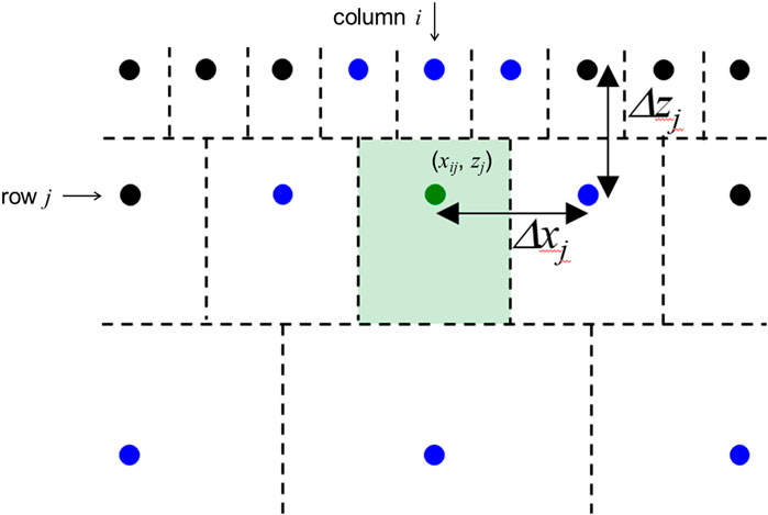
FIGURE 3. Interpolating points for a typical control volume (shaded).

Using the expressions for stress from Eq. 3, leads to

$f_x^S=\left(\lambda +2G\right)\underset{z_j-\frac{1}{2}\mathrm{\Delta }{z}_j}{\overset{z_j+\mathrm{\Delta }{z}_j}{{\displaystyle \int }}}\left({\frac{\partial u}{\partial x}|}_{x_{ij}-\frac{1}{2}\mathrm{\Delta }{x}_j}^{x_{ij}+\frac{1}{2}\mathrm{\Delta }{x}_j}\right)dz+\left(\lambda +G\right){\left({w\left(x,z\right)|}_{x_{ij}-\frac{1}{2}\mathrm{\Delta }{x}_j}^{x_{ij}+\frac{1}{2}\mathrm{\Delta }{x}_j}\right)}_{z_j-\frac{1}{2}\mathrm{\Delta }{z}_j}^{z_j+\mathrm{\Delta }{z}_j}+G\underset{x_{ij}-\frac{1}{2}\mathrm{\Delta }{x}_j}{\overset{x_{ij}+\frac{1}{2}\mathrm{\Delta }{x}_j}{{\displaystyle \int }}}\left({\frac{\partial u}{\partial z}|}_{z_j-\frac{1}{2}\mathrm{\Delta }{z}_j}^{z_j+\mathrm{\Delta }{z}_j}\right)dx(6)$

$f_z^S=\left(\lambda +2G\right)\underset{x_{ij}-\frac{1}{2}\mathrm{\Delta }{x}_j}{\overset{x_{ij}+\frac{1}{2}\mathrm{\Delta }{x}_j}{{\displaystyle \int }}}\left({\frac{\partial w}{\partial z}|}_{z_j-\frac{1}{2}\mathrm{\Delta }{z}_j}^{z_j+\mathrm{\Delta }{z}_j}\right)dx+\left(\lambda +G\right){\left({u\left(x,z\right)|}_{z_j-\frac{1}{2}\mathrm{\Delta }{z}_j}^{z_j+\mathrm{\Delta }{z}_j}\right)}_{x_{ij}-\frac{1}{2}\mathrm{\Delta }{x}_j}^{x_{ij}+\frac{1}{2}\mathrm{\Delta }{x}_j}+G\underset{z_j-\frac{1}{2}\mathrm{\Delta }{z}_j}{\overset{z_j+\mathrm{\Delta }{z}_j}{{\displaystyle \int }}}\left({\frac{\partial w}{\partial x}|}_{x_{ij}-\frac{1}{2}\mathrm{\Delta }{x}_j}^{x_{ij}+\frac{1}{2}\mathrm{\Delta }{x}_j}\right)dz(7)$

To approximate the value of each of the terms above, we introduce bi-quadratic interpolation functions according to:

$\begin{array}{l}{\varphi }_u\left(x,z\right)\equiv {\gamma }_T\left(\eta \right)\left[u_{2\left(i-1\right),j-1}{\alpha }_{TL}\left(\xi \right)+u_{2\left(i-1\right)+1,j-1}{\alpha }_{TM}\left(\xi \right)+u_{2i,j-1}{\alpha }_{TR}\left(\xi \right)\right]\\ +{\gamma }_M\left(\eta \right)\left[u_{i-1,j}{\alpha }_{ML}\left(\xi \right)+u_{i,j}{\alpha }_{MM}\left(\xi \right)+u_{i+1,j}{\alpha }_{MR}\left(\xi \right)\right]\\ +{\gamma }_B\left(\eta \right)\left[\begin{array}{cc}{u}_{\frac{i}{2},j}{\lambda }_L\left(\xi \right)+u_{\frac{i+2}{2},j}{\lambda }_R\left(\xi \right)& \text{if}i\text{is}\text{even}\\ u_{\frac{i-1}{2},j+1}{\alpha }_{BL}\left(\xi \right)+u_{\frac{i+1}{2},j}{\alpha }_{BM}\left(\xi \right)+u_{\frac{i+3}{2},j}{\alpha }_{BR}\left(\xi \right)& \text{if}i\text{is}\text{odd}\end{array}\right]\end{array}(8)$

$\begin{array}{l}{\varphi }_w\left(x,z\right)\equiv {\gamma }_T\left(\eta \right)\left[w_{2\left(i-1\right),j-1}{\alpha }_{TL}\left(\xi \right)+w_{2\left(i-1\right)+1,j-1}{\alpha }_{TM}\left(\xi \right)+w_{2i,j-1}{\alpha }_{TR}\left(\xi \right)\right]\\ +{\gamma }_M\left(\eta \right)\left[w_{i-1,j}{\alpha }_{ML}\left(\xi \right)+w_{i,j}{\alpha }_{MM}\left(\xi \right)+w_{i+1,j}{\alpha }_{MR}\left(\xi \right)\right]\\ +{\gamma }_B\left(\eta \right)\left[\begin{array}{cc}{w}_{\frac{i}{2},j}{\lambda }_L\left(\xi \right)+w_{\frac{i+2}{2},j}{\lambda }_R\left(\xi \right)& \text{if}i\text{is}\text{even}\\ w_{\frac{i-1}{2},j+1}{\alpha }_{BL}\left(\xi \right)+w_{\frac{i+1}{2},j}{\alpha }_{BM}\left(\xi \right)+w_{\frac{i+3}{2},j}{\alpha }_{BR}\left(\xi \right)& \text{if}i\text{is}\text{odd}\end{array}\right]\end{array}(9)$

where ${\varphi }_u\left(x,z\right)$ and ${\varphi }_w\left(x,z\right)$ represent the approximate behavior of the functions $u\left(x,z\right)$ and $w\left(x,z\right)$, respectively, in the vicinity of the node having row index j and, within that row, horizontal index i, where the first node (starting at the left) begins with an index value of 1 (Figure 2). Now ${\gamma }_T\left(\eta \right), {\gamma }_M\left(\eta \right)$ and ${\gamma }_B\left(\eta \right)$ are the three Lagrange interpolating polynomials associated with the set of three z-values equaling $z_{j-1}$, $z_j$ and $z_{j+1}$, where $\eta \equiv \frac{z-z_{j-1}}{\mathrm{\Delta }{z}_j}$. Similarly, for row indexes j−1, and j, there is a set of three Lagrange interpolating polynomials (α′s) associated with the three x-values nearest the (i, j) node with $\xi \equiv \frac{x-x_{i-1,j}}{\mathrm{\Delta }x}$ , where $x_{i-1,j}$ denotes the x coordinate of node i−1 of row j. (The subscript nomenclature on the individual interpolating functions is such that T, M, B denote top, middle and bottom, respectively, while L, M, R denote left, middle and right, respectively.) For the row index j + 1, there is either a set of two or three interpolating polynomials, depending upon whether node i is even or odd. The highlighted nodes (in blue) of Figure 3 show the set of nodal points used to establish the interpolating functions for a typical interior node with index i,j for odd i. It is clear, for even i, only the two nearest nodes in the row below are used as interpolating points. Note that ${\varphi }_u\left(x,y\right)$ and ${\varphi }_w\left(x,y\right)$ are formulated to take on precisely the corresponding nodal displacement values at each of the nodal locations.

For a typical interior node, it can be shown that the Lagrange interpolating polynomials are given by:

$\begin{array}{ccc}{\gamma }_T\left(\eta \right)=\frac{1}{3}\left(\eta -1\right)\left(\eta -3\right)& {\gamma }_M\left(\eta \right)=-\frac{1}{2}\eta \left(\eta -3\right)& {\gamma }_B\left(\eta \right)=\frac{1}{6}\eta \left(\eta -1\right)\end{array}$

$\begin{array}{cc}{\alpha }_{TL}\left(\xi \right)=2\left(\xi -1\right)\left(\xi -\frac{3}{2}\right){\alpha }_{TM}\left(\xi \right)=-4\left(\xi -\frac{1}{2}\right)\left(\xi -\frac{3}{2}\right)& {\alpha }_{TR}\left(\xi \right)=2\left(\xi -1\right)\left(\xi -\frac{1}{2}\right)\end{array}(10)$

$\begin{array}{cc}{\alpha }_{ML}\left(\xi \right)=\frac{1}{2}\left(\xi -1\right)\left(\xi -2\right){\alpha }_{MM}\left(\xi \right)=-\xi \left(\xi -2\right)& {\alpha }_{MR}\left(\xi \right)=\frac{1}{2}\xi \left(\xi -1\right)\end{array}$

$\begin{array}{cc}{\alpha }_{BL}\left(\xi \right)=\frac{1}{8}\left(\xi -1\right)\left(\xi -3\right){\alpha }_{BM}\left(\xi \right)=-\frac{1}{4}\left(\xi +1\right)\left(\xi -3\right)& {\alpha }_{BR}\left(\xi \right)=\frac{1}{8}\left(\xi +1\right)\left(\xi -1\right)\end{array}\left(i\text{odd}\right)$

$\begin{array}{cc}{\lambda }_{BL}\left(\xi \right)=-\frac{1}{2}\left(\xi -1\right)& {\lambda }_{BR}\left(\xi \right)=\frac{1}{2}\left(\xi +1\right)\left(i\text{even}\right)\end{array}$

Now, using these interpolating functions, the relationship between “spring” forces (Eq. 6 and Eq. 7) and nodal displacements can be determined via analytical integration, differentiation and evaluation. For a control volume element that is not typical, such as one situated in the second row of nodal elements and/or one having at least one of its boundaries coinciding with part of the slab boundary, the approach is the same, but with modified forms for the interpolating functions.

2.1.4 Matrix Formulation

The foregoing interpolation procedure gives rise to the following set of matrix equations:

$\begin{array}{c}\left\{f_x\right\}=\left[K_u\right]\left\{u\right\}+\left[C_{uw}\right]\left\{w\right\}\\ \left\{f_z\right\}=\left[C_{wu}\right]\left\{u\right\}+\left[K_w\right]\left\{w\right\}\end{array}(11)$

where: $\left\{f_x\right\}$ is the vector of all the externally applied nodal forces in the x-direction.

$\left\{f_z\right\}$ is the vector of all the externally applied nodal forces in the z-direction.

$\left\{u\right\}$ is the vector of all nodal displacements in the x-direction.

$\left\{w\right\}$ is the vector of all nodal displacements in the z-direction.

$\left[K_u\right]$ is the stiffness matrix relating applied nodal forces in the x-direction to the displacements in the x-direction.

$\left[C_{uw}\right]$ is the stiffness matrix relating applied nodal forces in the x-direction to the displacements in the z-direction.

$\left[K_w\right]$ is the stiffness matrix relating applied nodal forces in the z-direction to the displacements in the z-direction.

$\left[C_{wu}\right]$ is the stiffness matrix relating applied nodal forces in the z-direction to the displacements in the x-direction.

The above system of Eq. 11 contains two equations for each node, one for each of its two degrees of freedom. A contact problem is formulated by specifying, at each node, a value for either $f_x$ or $u$ and a value for either $f_z$ or $w$. The system of equations can then be solved for all unknown (i.e., un-prescribed) forces and displacements. In fact, in a manner previously described (Avlonitis et al., 2014) the equations can be re-ordered so that all of the equations involving prescribed displacements appear first. Then the matrices can be partitioned accordingly, so that the solutions for the unknown forces and unknown displacements may be written explicitly in terms of matrix operations.

2.2 Dynamic Simulation

2.2.1 Governing Equation

In many practical situations, one body is sliding over another while being driving by a spring (i.e., via a connection with a finite stiffness). Suppose, as illustrated in Figure 4, that the pin of Figure 1 is being driven horizontally by a stage that couples to the pin via a spring of stiffness, k, and that the system experiences linear viscous damping with damping coefficient c. Thus, the spring and damper exert the driving force on the pin, which has mass m and experiences a displacement x_p relative to the origin. The macroscopic concept of static friction says that the pin will be “stuck” to the counter surface until there is sufficient driving force to initiate sliding of the pin across the surface. Now suppose the stage displacement is given by $x_S=V_{o}t$ and the pin starts at rest at x = 0 at t = 0. The governing equation for the pin position is given as

$m\ddot{x_p}=k\left(V_{o}t-x_p\right)+c\left(V_o-\dot{x_p}\right)-F\left(t\right)(12)$

where the time varying friction force F(t) is based on the results of the simulation of nanoscale friction from the first part of the mathematical modelling (Section 2.1), the details of which are described in the next section.

FIGURE 4

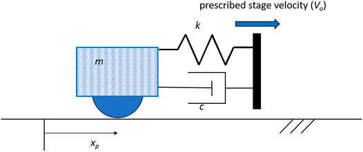
FIGURE 4. Configuration of system considered in dynamic simulation.

It is well known (Thomson, 1972) that a one degree-of-freedom spring-mass-damper system can be categorized as underdamped, critically damped, or overdamped depending on the damping ratio, $\zeta$, which is given as $\zeta =c/\left(2m{\omega }_n\right)$ where ${\omega }_n$ is the (undamped) natural frequency and is equal to $\sqrt{k/m}$. In this paper we consider an underdamped system, which means that the damping ratio is less than unity.

2.2.2 Friction Force Determination

Whereas, during the quasistatic nanoscale simulation, the pin translates in a single direction, there is, within the dynamic simulation, the freedom for the pin to assume negative velocities. Thus, the friction force is not a true function of position. Rather, because of slip, there is hysteresis. In fact, one expects the behavior to be similar to what happens to a specimen in a simple tension test (Dowling, 1993). In the simplest case, the stress grows in proportion to the strain and then a stress plateau is reached. During unloading the stress immediately decreases below the value of the stress plateau. Hence, there will be more than one value of strain corresponding to a particular value of stress, depending upon whether the point is part of the loading curve or the unloading curve. In anticipation of such hysteresis, we construct the nanoscale friction force function in the following manner:

$F\left(t\right)=\{\begin{array}{cc}\min \left(K\left(x\left(t\right)-x_R\right),\tilde{F}\left(x\left(t\right)\right)\right)& x>x_R\\ -\min \left(K\left(\left|x\left(t\right)-x_R\right|\right),\tilde{F}\left(x\left(t\right)\right)\right)& x<x_R\end{array}(13)$

where K is the lateral surface stiffness (which may be determined from the stiffness matrices in Eq. 11, or through analysis of the force response in the absence of slip), $x_R$ is the “relaxation point,” which is defined as the lateral position of the pin corresponding to zero friction force being exerted by the elastic slab, $\tilde{F}\left(x\right)$ is the friction force profile arising from the nanoscale friction simulation. Note that $x_R$ changes whenever there is a slip event and is analogous to the change in permanent strain whenever there is plastic deformation in a simple tension test. Therefore, we can define the relaxation point according to:

$x_R=x\left(t\right)-F\left(t\right)/K(14)$

While the connection between Eq. 13 and Eq. 14, appears to be circular, the proper interpretation is as follows: $x_R$ starts out with a particular value, which is used in Eq. 13. So long as the first argument to the “min” function is less than or equal to $\tilde{F}\left(x\left(t\right)\right),$ the RHS of Eq. 14 yields $F\left(t\right)= K\left(x\left(t\right)-x_R\right)$ and the use of this result in Eq. 14 assigns $x_R=x_R$. Hence, in this case, there is no change in the value of the relaxation point. On the other hand, as soon as $K\left(x\left(t\right)-x_R\right)$ exceeds $\tilde{F}\left(x\left(t\right)\right)$ at a particular time step, we get from Eq. 13 that $F\left(t\right)=\tilde{F}\left(x\left(t\right)\right)$ so that Eq. 14 leads to $x_R=x\left(t\right)-\tilde{F}\left(x\left(t\right)\right)/K$. Therefore, the relaxation point changes. Now the surface stiffness, K, may be expressed as,

$K=\frac{d\tilde{F}\left({\delta }_p\right)}{d{\delta }_p}(15)$

where the derivative is evaluated by considering, in the nanoscale simulation, changes in friction force during sufficiently small displacements that no slip occurs.

It is of interest to incorporate the nanoscale friction results, which involve total pin translation distances that are hundreds of nanometers, into dynamic simulations that involve sliding distances that are several orders of magnitude larger. To do this, we make the assumption of spatial periodicity in the “steady-state” portion of the nanoscale friction function $\tilde{F}\left(x\right)$, with the spatial period being about the size of the sliding distance used for the nanoscale simulation, its particular value dependent on the form of $\tilde{F}\left(x\right)$.

2.2.3 Numerical Integration

The motion of the pin as well as the friction and spring forces are determined from numerical integration of Eq. 12. For this purpose, we employ the well-known fourth order Runge-Kutta integration scheme. The pin is assumed to be initially at rest x = 0 at t = 0.

3 Results and Discussion

Simulations were performed to obtain nanoscale force vs displacement curves (Figure 1) and to investigate the static and kinetic friction behavior of the interface when the pin is driven dynamically by way of a constant-velocity stage and coupling spring (Figure 4).

3.1 Model Validation

To investigate the computation accuracy of the numerical approach, we simulated the normal contact of a rigid flat punch. Figure 5 shows the comparison between the analytical solution for the pressure distribution, given by $p\left(x\right)= p_o/\sqrt{1-{\left(x/a\right)}^2}$ (Johnson, 1985) within the contact zone, and that from the current work for the case of n_x = 129 (i.e., 129 nodal points along the slab surface). For the numerical simulation, the bottom surface of the test slab was prescribed to be fixed in its vertical position and to exert no friction, while the contact points in the interface (within radius a) were prescribed to have uniform downward displacement and also be frictionless. As observed, there is excellent agreement between the numerical solution and the exact result.

FIGURE 5

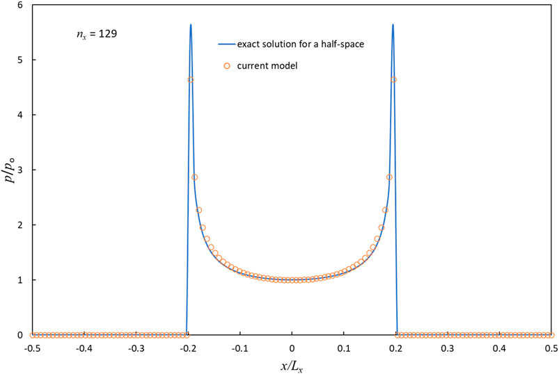
FIGURE 5. Comparison of the shape of the pressure distribution for current model with that of the exact solution $p\left(x\right)= p_o/\sqrt{1-{\left(x/a\right)}^2}$ for a rigid flat punch indenting a half-space. (Infinite values in the exact solution at |x| = a are omitted.)

3.2 Friction Force vs Displacement—Nanoscale Friction

3.2.1 Friction Force Profile

Figure 6 shows the friction force, F, normalized by the compressive load W, vs dimensionless pin displacement for two values of intrinsic static friction coefficient (µ_i). For this simulation, we used n_x = 129, a slab aspect ratio (L_z/L_x) equal to unity and a normalized pin radius R/L_x equal to 200. For µ_i =0.5, it is observed that the friction increases nearly linearly with increasing pin displacement for the first portion of the force record until reaching a value of around 0.28, after which the friction hovers “noisily” about this value for increasing pin displacement. Qualitatively similar results occur for the lower value of µ_i but with a lower “steady-state” value and a thinner band of variation within the steady-state region. As observed in Figure 6, the mean values of the plateaus in F/W are about 56% of their respective values of the intrinsic static friction coefficient.

FIGURE 6

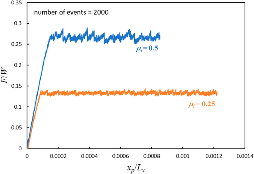
FIGURE 6. Normalized, nanometer-scale friction force (friction force over normal force) as a function of dimensionless horizontal pin displacement.

Each of the friction records in Figure 6 corresponds to 2000 “events”, an event corresponding to the minimum pin displacement that triggers one of three occurrences: 1) a node is forced to be released (i.e., remaining in contact would violate pressure non-negativity at that node) 2) a node is slipped (i.e., remaining stuck would violate $\tau \le {\mu }_{i}p$), or 3) a node must be moved from non-contact to contact (i.e., remaining at zero pressure would violate non-interpenetration). It should be noted that the overwhelming majority of events are slips. For example, in the case of µ_i =0.5, 1,952 of the 2,000 events were associated with nodal slip, while 44 were associated with nodal release, with the remaining four corresponding to nodes coming into contact. It is also noted that it was necessary to define a lower bound for the minimum pin displacement to avoid getting trapped in a never-ending loop of ever diminishing pin displacements. For the results shown in the present work, the threshold for recognizing an event was a pin displacement equal to the minimum horizontal grid spacing [i.e., L_x/(n_x −1)] divided by 10⁶.

3.2.2 Nanoscale Pin Displacement

It should be noted, that for a given choice of Poisson’s ratio (we have selected a value of 1/3), the ratio of friction force to normal load (F/W) is independent of the elastic modulus. Moreover, as can be demonstrated from dimensional analysis, for a given value of Poisson’s ratio and choice of µ_i, the relationship between F/W and δ_p/L_x depends only the slab aspect ratio L_z/L_x, the normalized pin radius R/L_x and the number of nodes applied to the top surface of the slab. Therefore, to interpret the results of Figure 6 as corresponding to the nanoscale we must first define appropriate lateral dimensions for the slab. In this vein, we choose L_x = L_z = 1 mm, so that the total pin displacements of Figure 6 become about 0.9 and 1.3 µm for µ_i = 0.5 and µ_i = 0.25, respectively. Considering that each force record corresponds to 2000 incremental displacements of the pin, we see that the average plate displacement per triggering event would be smaller than 1 nm. Along these lines, Figure 7 shows the dimensionless pin displacement for each event as well as the cumulative pin displacement for the case of µ_i = 0.5. As observed, a square slab with a side length of 1 mm gives rise to many sub-nanometer pin displacements that induce slip.

FIGURE 7

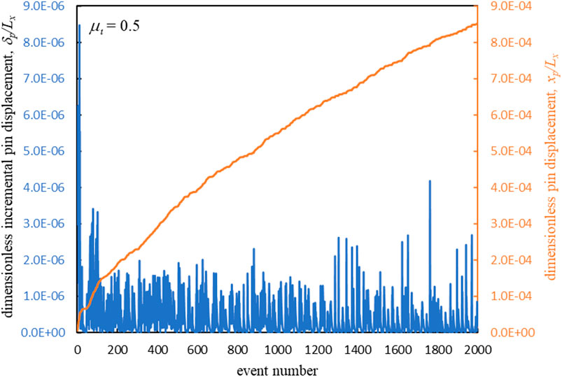
FIGURE 7. Incremental and cumulative pin displacement as a function of event number. An event is defined as a slip, release or re-establishment of contact at a node.

3.2.3 Effect of Grid Resolution

Figure 8 shows how the mean dimensionless pin displacement varies with increasing the number of nodes comprising the contacting surface of the slab. Here we show results for two values of pin radius. It is observed that increasing the number of nodes results in an overall power law trend of reducing mean plate displacement per triggering event. Based on these results, it seems plausible that, in the limit of infinite resolution (i.e., the continuum limit), the average slip distance will be zero, suggesting that the interface will slide smoothly at a single kinetic force value. However, this mathematical result is unlikely to match reality, owing to the physical length scale associated with atomic lattice positions. That is, two opposing surface regions are “stuck” together when there is a significant energy barrier to relative lateral motion. Such an energy barrier arises from the atoms of one surface interacting with the electrostatic field of the other. Such a field almost invariably has spatial fluctuations in force that correspond to characteristic lattice dimensions (Binnig, 1987; Mate et al., 1987; Mate et al., 1988; Meyer et al., 1988; Kaneko, 1989; Singer, 1994; Harrison et al., 1995; Krim, 1996; Sorensen et al., 1996; Zhang and Tanaka, 1997; Bennewitz et al., 1999; Bennewitz et al., 2001; Streator, 2019). Therefore, it may not be meaningful to increase the grid resolution beyond that which induces average slip distances below around 0.5 nm.

FIGURE 8

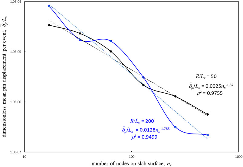
FIGURE 8. Scaling of average pin displacement per event step as a function of the grid resolution.

3.3 Macroscopic Static and Kinetic Friction

We now simulate the sliding process, by integrating Eq. 12 subject to the rules expressed by Eq. 13 and Eq. 14. Recall that, whereas the nanoscale friction function $\tilde{F}\left(x\left(t\right)\right)$ is obtained over a short distance (e.g., ∼1 µm), we impose periodicity on the steady-state portion of the friction record, with a spatial period equal to the length of this portion. This extension of the nanoscale force response enables much larger sliding distances to be studied. For this dynamic simulation, the following parameter values are used (see Figure 4):

• spring stiffness, k = 200 kN/m

• damping ratio, $\zeta$ = 0.1

• stage velocity, V_o = 2 mm/s

• pin mass, m = 0.5 kg

• integration time step, Δt = 100 ns

To convert the normalized results for the nanoscale friction into physical quantities, the following parameters were assigned:

• width of slab (L_x) = 1 mm

• vertical thickness of slab (L_z) = 1 mm

• depth of slab (L_y) = 1 cm

• intrinsic coefficient of friction (µ_i) = 0.25, or 0.5

• radius of curvature of pin tip (R) = 50 cm or 200 cm

• normal load (W) = 100 N

• elastic constants for slab: G = 10 GPa, ν = 1/3

Figure 9 shows how the spring force varies over time when the system of Figure 4 experiences the force profile defined by extensions of the nanoscale force records of Figure 6. The spring force is of particular interest because that is the usual quantity from which the static and kinetic coefficients of friction are determined experimentally. Precisely speaking, the static friction force must balance the sum of the spring force and the force of the damper. In many practical situations the contribution from damping can be ignored in determining the static coefficient of friction. For the chosen parameters of the spring-mass-damper system and with an intrinsic friction coefficient of 0.5, the damping force exerted on a stationary pin is given by $F_{\text{damping}}=c{V}_o=\left(2\zeta \sqrt{mk}\right)V_o=2\left(0.1\right)\sqrt{\left(0.5\text{kg}\right)\left(2\times {10}^5\frac{\text{N}}{\text{m}}\right)}\left(.002\frac{\text{m}}{\text{s}}\right)=0.13\text{N}$,

FIGURE 9

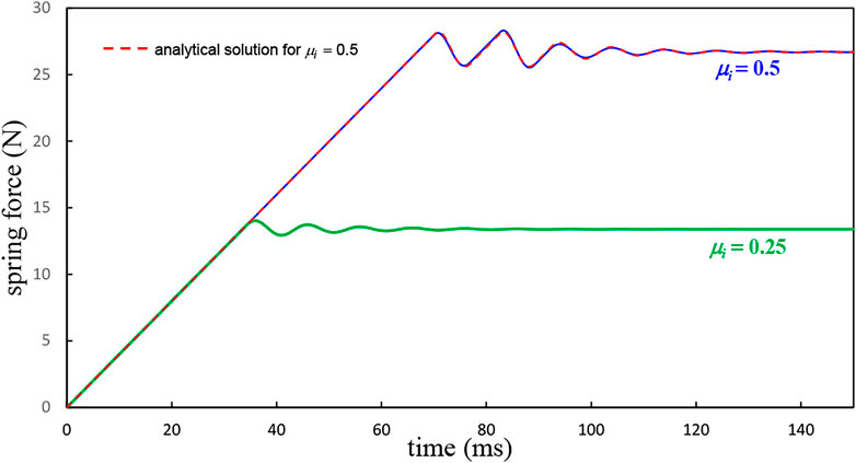
FIGURE 9. Force in coupling spring as a function of time while pin is being driven by a stage that translates at a constant velocity of 2 mm/s, for two different intrinsic static coefficients of friction. In each case pin experiences a position-dependent friction force defined by the nanometer-scale friction function per Figure 6.

which is less than 1% of the peak spring force. As observed, for both values of intrinsic coefficient of static friction, the spring force grows linearly until giving way to a damped sinusoidal variation. In the case of µ_i = 0.5, the pin exhibits two clear stick phases, whereas, for µ_i = 0.25, only one stick phase is observed. Also displayed in Figure 9 are the results of an analytical model arising from a closed form solution of Eq. 12, using a single kinetic coefficient of friction throughout (µ_k = 0.267), along with two static coefficients of friction (µ_s = 0.282 for t ≤ 89 ms and µ_s = 0.272 for t > 89 ms). The spring force calculated from this model is found to agree remarkably well with the results of the more extensive numerical solution, which incorporates the nanoscale friction force profile. The particular set of friction coefficient values was chosen to provide the best match with the numerical solution. For clarity, the analytical result for the spring-mass-damper system is now presented. During a stick phase, we have,

$x_p\left(t\right)=x_{\text{stick}}\equiv x_p\left(t_{\text{stick}}\right)$

$V_p\left(t\right)=0(16)$

$F_{\text{spring}}=k\left(V_{o}t-x_{\text{stick}}\right)$

while during a slip we get,

$x_p\left(t\right)=V_{o}t-\frac{{\mu }_{k}W}{k}+\text{exp}\left[-\zeta {\omega }_n\left(t-t_{\text{slip}}\right)\right]\left\{\left[\frac{{\mu }_{k}W}{k}+x_{\text{stick}}-V_o{t}_{\text{slip}}\right]\left[\cos {\omega }_d\left(t-t_{\text{slip}}\right)+\zeta \frac{{\omega }_n}{{\omega }_d}\sin {\omega }_d\left(t-t_{\text{slip}}\right)\right]-\frac{V_o}{{\omega }_d}\sin {\omega }_d\left(t-t_{\text{slip}}\right)\right\}$

$V_p\left(t\right)=V_o+\exp \left[-\zeta {\omega }_n\left(t-t_{\text{slip}}\right)\right]\left\{-V_o\cos {\omega }_d\left(t-t_{\text{slip}}\right)+\left(V_o{t}_{\text{slip}}-x_{\text{stick}}-\frac{{\mu }_{k}W}{k}\right)\frac{{\omega }_d}{1-{\zeta }^2}\sin {\omega }_d\left(t-t_{\text{slip}}\right)\right\}(17)$

$F_{\text{spring}}={\mu }_{k}W-\text{exp}\left[-\zeta {\omega }_n\left(t-t_{\text{slip}}\right)\right]\left\{\left[{\mu }_{k}W+k\left(x_{\text{stick}}-V_o{t}_{\text{slip}}\right)\right]\left[\cos {\omega }_d\left(t-t_{\text{slip}}\right)+\zeta \frac{{\omega }_n}{{\omega }_d}\sin {\omega }_d\left(t-t_{\text{slip}}\right)\right]-\frac{k{V}_o}{{\omega }_d}\sin {\omega }_d\left(t-t_{\text{slip}}\right)\right\}$

where ${\omega }_n$ is the undamped natural frequency, ${\omega }_d$ is the damped natural frequency $\left(={\omega }_n\sqrt{1-{\zeta }^2}\right)$, $t_{\text{slip}}$ is the time of slip onset from the most recent stick phase, and $x_{\text{stick}}$ is the (constant) position of the pin during the most recent stick phase. Since, during stick, the friction force reacts to the driving force to prevent pin motion, slip onset occurs when the friction force reaches its limit:

${\mu }_{s}W=k\left(V_o{t}_{\text{slip}}-x_{\text{stick}}\right)+c{V}_o(18)$

$t_{\mathrm{slip}}=\frac{{\mu }_{s}W}{k{V}_o}-\frac{c}{k}+\frac{x_{\mathrm{stick}}}{V_{\mathrm{o}}}(19)$

Finally, re-sticking from a slip phase occurs if and when the pin speed vanishes.

Figure 10 shows some details of the motion for the case of µ_i = 0.5. For the first 70 ms or so of stage motion, the pin remains stuck to the slab, as evidenced by the essentially zero pin displacement. The pin velocity, on the other hand reveals that there is some activity even from the very beginning, as low-amplitude, high-frequency fluctuations are observed. Then, at the point of macroscopic slip (≈70 ms), there is a sudden increase in the velocity of the pin. The velocity record reveals that there are actually two re-sticks (as opposed to the apparent single re-stick shown by the record of spring force). Ultimately the pin speed tends toward a value of 2 mm/s which is the value of the stage velocity. Also displayed in Figure 10 are the analytical curves based on Eq. 16. Both pin velocity and pin displacement show strong agreement with the extensive numerical simulation.

FIGURE 10

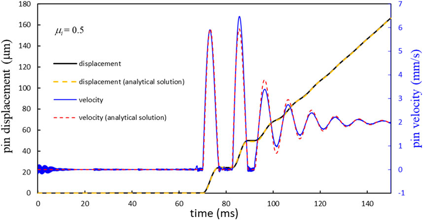
FIGURE 10. Motion of the pin during dynamic simulation.

Additional insight as to the interplay between nanoscale effects and macroscale observations can be gained from Figure 11, which shows the actual (instantaneous) friction force exerted on the pin. At the beginning of the process, there are fluctuations in the force due to elastic vibrations of the slab as the slab responds to sudden lateral loading on the pin (i.e., the stage motion begins impulsively). These oscillations largely die out after 15 ms or so. For the remaining macroscopic stick phase, which extends until about 70 ms, there are intermittent, small-amplitude “bursts” of friction force oscillation. Each of these bursts is triggered by a sudden (but small) drop in the instantaneous friction force, which arises from local, nanoscale slip in the interface. The sudden drop in friction force causes the pin to translate forward, inducing a vibratory response of the slab. At low lateral loads, pin sliding is quickly arrested as the interface can exert an overall increasing friction force as the pin traverses the slab. Ultimately, a nanoslip occurs at a sufficiently high force level that the overall trend of the friction is flat with respect to relative displacement. At this point, the pin experiences macroscopic slip. As seen in Figure 11, the slip phase is characterized by high-frequency fluctuations in the friction force. This result is to be expected because, as demonstrated in Figure 6, significant variations in friction can occur over sub-nanometer length scales. Therefore, sliding speeds of a few mm/s mean that nanometer length scales are traversed in microseconds.

FIGURE 11

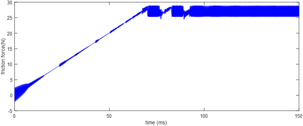
FIGURE 11. Instantaneous friction force experienced by the pin as it is being driven the by stage for the case of µ_i = 0.5.

The results depicted in Figures 9–11 provide a simple, plausible explanation for the ubiquitous existence of static and kinetic friction coefficients, the latter generally being smaller than the former: The static coefficient of friction corresponds to a major peak in the nanoscale friction force profile, while the kinetic coefficient of friction corresponds to the average nanoscale friction force during its steady-state phase.

4 Conclusion

A two-part numerical simulation was performed to investigate the sliding behavior of a rigid, curved pin against a stationary elastic slab, which experienced plane strain deformation. For the nanoscale friction model, a multi-scale grid based on a binary hierarchy was implemented on the elastic slab to account for its deformation. Bi-quadratic interpolating functions were used to determine the four stiffness matrices relating deformation to force. The pin was given a prescribed position, which was changed incrementally in accordance with the minimum displacement needed to cause either a nodal slip, a nodal release, or a new nodal contact. Slip was imposed at a node whenever the nodal shear stress would otherwise be greater than the product of an assumed intrinsic static coefficient of friction and the nodal pressure. Nodal release was imposed whenever a node would otherwise develop a negative pressure and new nodal contact was established whenever a node would otherwise penetrate the pin. A nanoscale friction function was developed by computing the equilibrium friction force as a function of pin displacement.

In the second part of the simulation, the pin was coupled via a spring to a stage that moved at a constant velocity, and a dynamic simulation of the pin motion was conducted. The instantaneous friction force was determined by the nanoscale friction force vs displacement function. Key findings of the study are that:

1) The stick phase of classic stick-slip behavior is characterized by many micro-slips of short duration.

2) Sliding is characterized by high frequency fluctuations in instantaneous friction force.

3) Both the macroscopic static and kinetic coefficients of friction are much less than the intrinsic static friction coefficient.

4) The static coefficient of friction is associated with a major peak of the nanoscale friction function.

5) The kinetic coefficient of friction is associated with the average of the steady-state phase of the nanoscale friction function.

Data Availability Statement

The raw data supporting the conclusion of this article will be made available by the authors, without undue reservation.

Author Contributions

JS is the sole author.

Conflict of Interest

The author declares that the research was conducted in the absence of any commercial or financial relationships that could be construed as a potential conflict of interest.

Publisher’s Note

All claims expressed in this article are solely those of the authors and do not necessarily represent those of their affiliated organizations, or those of the publisher, the editors and the reviewers. Any product that may be evaluated in this article, or claim that may be made by its manufacturer, is not guaranteed or endorsed by the publisher.

References

Amontons, G. (1699). On the Resistance Orignating in Machines. Mem. Acad. Roy., 206–227.

Google Scholar

Avlonitis, M., Kalaitzidou, K., and Streator, J. (2014). Investigation of Friction Statistics and Real Contact Area by Means of a Modified OFC Model. Tribology Int. 69, 168–175. doi:10.1016/j.triboint.2013.07.018

CrossRef Full Text | Google Scholar

Bennewitz, R., Gyalog, T., Guggisberg, M., Bammerlin, M., Meyer, E., and Güntherodt, H.-J. (1999). Atomic-scale Stick-Slip Processes on Cu(111). Phys. Rev. B 60 (16), R11301–R11304. doi:10.1103/physrevb.60.r11301

CrossRef Full Text | Google Scholar

Bennewitz, R., Meyer, E., Bammerlin, M., Gyalog, T., and Gnecco, E. (2001). “Atomic-scale Stick Slip,” in Fundamentals of Tribology and Bridging the Gap between the Macro-and Micro/Nanoscales. Editor B. Bhushan (Dordrecht: Springer), 10, 53–66. doi:10.1007/978-94-010-0736-8_4

CrossRef Full Text | Google Scholar

Binnig, G. K. (1987). Atomic-Force Microscopy. Phys. Scr. T19a, 53–54. doi:10.1088/0031-8949/1987/t19a/008

CrossRef Full Text | Google Scholar

Braun, O. M., Barel, I., and Urbakh, M. (2009). Dynamics of Transition from Static to Kinetic Friction. Phys. Rev. Lett. 103 (19), 194301. doi:10.1103/PhysRevLett.103.194301

PubMed Abstract | CrossRef Full Text | Google Scholar

Braun, O. M., and Peyrard, M. (2008). Modeling Friction on a Mesoscale: Master Equation for the Earthquakelike Model. Phys. Rev. Lett. 100 (12), 125501. doi:10.1103/PhysRevLett.100.125501

PubMed Abstract | CrossRef Full Text | Google Scholar

Braun, O. M., and Röder, J. (2002). Transition from Stick-Slip to Smooth Sliding: An Earthquakelike Model. Phys. Rev. Lett. 88 (9), 096102. doi:10.1103/PhysRevLett.88.096102

PubMed Abstract | CrossRef Full Text | Google Scholar

Braun, O. M. (2010). Bridging the Gap between the Atomic-Scale and Macroscopic Modeling of Friction. Tribol Lett. 39 (3), 283–293. doi:10.1007/s11249-010-9648-7

CrossRef Full Text | Google Scholar

Brown, S. R., Scholz, C. H., and Rundle, J. B. (1991). A Simplified Spring-Block Model of Earthquakes. Geophys. Res. Lett. 18 (2), 215–218. doi:10.1029/91gl00210

CrossRef Full Text | Google Scholar

Burridge, R., and Knopoff, L. (1967). Model and Theoretical Seismicity. Bull. Seismological Soc. America 57 (3), 341–371. doi:10.1785/bssa0570030341

CrossRef Full Text | Google Scholar

Cao, P., Dahmen, K. A., Kushima, A., Wright, W. J., Park, H. S., Short, M. P., et al. (2018). Nanomechanics of Slip Avalanches in Amorphous Plasticity. J. Mech. Phys. Sol. 114, 158–171. doi:10.1016/j.jmps.2018.02.012

CrossRef Full Text | Google Scholar

Coulomb, C. A. (1785). The Theory of Simple Machines. Mem. Math. Phys. Acad. Sci. 10, 161–331.

Google Scholar

Dahmen, K. A. (2017). “Mean Field Theory of Slip Statistics,” in Avalanches in Functional Materials and Geophysics. Editors E. Salje, A. Saxena, and A. Planes (Cham: Springer), 19–30. doi:10.1007/978-3-319-45612-6_2

CrossRef Full Text | Google Scholar

De Moerlooze, K., Al-Bender, F., and Van Brussel, H. (2010). A Generalised Asperity-Based Friction Model. Tribol Lett. 40 (1), 113–130. doi:10.1007/s11249-010-9645-x

CrossRef Full Text | Google Scholar

Dong, Y. L., Li, Q. Y., and Martini, A. (2013). Molecular Dynamics Simulation of Atomic Friction: A Review and Guide. J. Vacuum Sci. Technol. A 31 (3), 030801. doi:10.1116/1.4794357

CrossRef Full Text | Google Scholar

Dowling, N. E. (1993). Mechanical Behavior of Materials : Engineering Methods for Deformation, Fracture, and Fatigue. Englewood Cliffs, N.J.: Prentice-Hall, xxiv, 773.

Google Scholar

Filippov, A. E., and Popov, V. L. (2010). Modified Burridge-Knopoff Model with State Dependent Friction. Tribology Int. 43 (8), 1392–1399. doi:10.1016/j.triboint.2010.01.010

CrossRef Full Text | Google Scholar

Gutenberg, B., and Richter, C. F. (1955). Magnitude and Energy of Earthquakes. Nature 176 (4486), 795. doi:10.1038/176795a0

CrossRef Full Text | Google Scholar

Harrison, J. A., White, C. T., Colton, R. J., and Brenner, D. W. (1995). Investigation of the Atomic-Scale Friction and Energy Dissipation in diamond Using Molecular Dynamics. Thin Solid Films 260 (2), 205–211. doi:10.1016/0040-6090(94)06511-x

CrossRef Full Text | Google Scholar

Haskell, P. T. (1961). “Insect Sounds,” in Aspects of Zoology Series (Chicago: Quadrangle Books), viii, 189.

Google Scholar

Helmholtz, H. V., and Ellis, A. J. (1954). On the Sensations of Tone as a Physiological Basis for the Theory of Music. 2d English ed. New York: Dover Publications, xix, 576.

Google Scholar

Ioannidis, P., Brooks, P. C., Barton, D. C., and Nishiwaki, M. (2002). “Brake System Noise and Vibration - A Review,” in Braking 2002: From the Driver to the Road (Leeds, United Kingdom: Transportation Research Laboratory), 53–73.

Google Scholar

Johnson, K. L. (1985). Contact Mechanics. Cambridge Cambridgeshire; New York: Cambridge University Press, xi, 452.

Google Scholar

Kaneko, R. (1989). Scanning Tunneling Microscopy and Atomic Force Microscopy - Approach to Micro-Tribology. J. Jpn. Soc. Tribologists 34 (1), 19–22.

Google Scholar

Kato, S., Yamaguch, K., and Matsubay, T. (1974). Stick-Slip Motion of Machine-Tool Slideway. Mech. Eng. 96 (1), 56. doi:10.1115/1.3438365

CrossRef Full Text | Google Scholar

Krim, J. (1996). Atomic-scale Origins of Friction. Langmuir 12 (19), 4564–4566. doi:10.1021/la950898j

CrossRef Full Text | Google Scholar

Mate, C. M., Erlandsson, R., McClelland, G. M., and Chiang, S. (1988). Summary Abstract: Atomic Force Microscopy Studies of Frictional Forces and of Force Effects in Scanning Tunneling Microscopy. J. Vacuum Sci. Technol. A: Vacuum, Surf. Films 6 (3), 575–576. doi:10.1116/1.575167

CrossRef Full Text | Google Scholar

Mate, C. M., McClelland, G. M., Erlandsson, R., and Chiang, S. (1987). Atomic-Scale Friction of a Tungsten Tip on a Graphite Surface. Phys. Rev. Lett. 59 (17), 1942–1945. doi:10.1103/physrevlett.59.1942

PubMed Abstract | CrossRef Full Text | Google Scholar

Meyer, E., et al. (1988). Applications of the Atomic Force Microscope. Helvetica Physica Acta 61 (1-2), 179.

Google Scholar

Olami, Z., Feder, H. J. S., and Christensen, K. (1992). Self-organized Criticality in a Continuous, Nonconservative Cellular Automaton Modeling Earthquakes. Phys. Rev. Lett. 68 (8), 1244–1247. doi:10.1103/physrevlett.68.1244

PubMed Abstract | CrossRef Full Text | Google Scholar

Patek, S. N. (2001). Spiny Lobsters Stick and Slip to Make Sound. Nature 411 (6834), 153–154. doi:10.1038/35075656

PubMed Abstract | CrossRef Full Text | Google Scholar

Persson, B. N. J. (1995). Theory of Friction: Stress Domains, Relaxation, and Creep. Phys. Rev. B 51 (19), 13568–13585. doi:10.1103/physrevb.51.13568

PubMed Abstract | CrossRef Full Text | Google Scholar

Singer, I. L. (1994). Friction and Energy Dissipation at the Atomic Scale: A Review. J. Vacuum Sci. Technol. A: Vacuum, Surf. Films 12 (5), 2605–2616. doi:10.1116/1.579079

CrossRef Full Text | Google Scholar

Smith, J., and Woodhouse, J. (2000). The Tribology of Rosin. J. Mech. Phys. Sol. 48 (8), 1633–1681. doi:10.1016/s0022-5096(99)00067-8

CrossRef Full Text | Google Scholar

Sorensen, M. R., Jacobsen, K. W., and Stoltze, P. (1996). Simulations of Atomic-Scale Sliding Friction. Phys. Rev. B Condens Matter 53 (4), 2101–2113. doi:10.1103/physrevb.53.2101

PubMed Abstract | CrossRef Full Text | Google Scholar

Stewart, D. G., and Hunt, J. B. (1970). Relaxation Oscillations in a Machine Tool Slideway. Ind. Lubrication Tribology 22 (8), 208.

Google Scholar

Streator, J. L. (2019). Nanoscale Friction: Phonon Contributions for Single and Multiple Contacts. Front. Mech. Eng. 5, 23. doi:10.3389/fmech.2019.00023

CrossRef Full Text | Google Scholar

Thomson, W. T. (1972). Theory of Vibration with Applications. Englewood Cliffs, N.J.: Prentice-Hall, x, 467.

Google Scholar

Zhang, D., Dahmen, K. A., and Ostoja-Starzewski, M. (2017). Scaling of Slip Avalanches in Sheared Amorphous Materials Based on Large-Scale Atomistic Simulations. Phys. Rev. E 95 (3), 032902. doi:10.1103/PhysRevE.95.032902

PubMed Abstract | CrossRef Full Text | Google Scholar

Zhang, L., and Tanaka, H. (1997). Towards a Deeper Understanding of Wear and Friction on the Atomic Scale-A Molecular Dynamics Analysis. Wear 211 (1), 44–53. doi:10.1016/s0043-1648(97)00073-2

CrossRef Full Text | Google Scholar

Zheng, S., Urueña, J. M., Dunn, A. C., Uhl, J. T., and Dahmen, K. A. (2020). Similarity of Internal and External Friction: Soft Matter Frictional Instabilities Obey Mean Field Dissipation through Slip Avalanches. Phys. Rev. Res. 2 (4), 042016. doi:10.1103/physrevresearch.2.042016

CrossRef Full Text | Google Scholar