 Yue Li
 Ji Hao1,2
 Caiyun Jin
 Zigeng Wang
95% of researchers rate our articles as excellent or good
Learn more about the work of our research integrity team to safeguard the quality of each article we publish.
Find out more
ORIGINAL RESEARCH article
Front. Mater. , 08 February 2021
Sec. Computational Materials Science
Volume 7 - 2020 | https://doi.org/10.3389/fmats.2020.603154
This article is part of the Research Topic Molecular Simulation on Cementitious Materials: From Computational Chemistry Method to Application View all 12 articles
The discrete element method (DEM) was used to establish the slump model and J-Ring model of concrete to describe the flow behavior in the slump test and J-Ring test. Then, the contact parameters of particle-particle and particle-geometry for the concrete DEM model, including restitution coefficient, rolling friction coefficient, static friction coefficient, and surface energy, were measured. In order to avoid the influence of the shape and size of the aggregate, this paper used high-precision glass spheres as the aggregate of the concrete for meso-calibration test, slump test, and J-Ring test. Comparing the simulation results of DEM model with slump test result, a very high agreement between the initial stage, the rapid flow stage, and the slow flow stage of the slump flow–time curve can be found as well as the final slump and slump flow. Moreover, similar to the slump DEM model, the DEM models of J-Ring test, V-funnel test, and U-channel test were established to study the passing ability and filling ability of concrete with outstanding accuracy. Therefore, the concrete DEM model with contact parameters and JKR model can be adopted to study the flow behavior of the fresh concrete.
Fresh concrete is a kind of complex composite material with highly uneven composition and structure. The trajectory of aggregate particles in fresh concrete greatly affects the flow behavior of concrete. Under the influence of aggregate particles, fresh concrete shows a flow behavior similar to particle flow (Hou et al., 2017). Considering the non-uniformity of fresh concrete on the meso level, the discrete element method (DEM) can truly simulate the flow behavior of the fresh concrete (Mechtcherine et al., 2013).
In recent years, the DEM has been widely used in the numerical simulation of fresh concrete. A variety of DEM contact models of fresh concrete have been proposed. Shyshko and Mechtcherine (2008) and Shyshko and Mechtcherine (2013) obtained the force-displacement relationship between the particles according to the experiments, establishing the interaction model of adjacent particles in the vertical direction, then directly introducing the model to establish a DEM model of fresh concrete with different workability. Finally, extensive simulations were conducted to study the effects of various model parameters on the numerical simulation results of the slump test. Guo et al. (2010) used the DEM and rheological model to simulate the workability test of fresh concrete by proposing the determination of the DEM parameters of the concrete (spring coefficient, friction coefficient, contact thickness, and damping coefficient). Remond and Pizette (2014) implemented a hard-core soft-shell DEM model to simulate concrete flowability. The fresh concrete was described as an assembly of composite particles made of spherical hard grains representing coarse aggregates surrounded by concentric spherical layers representing mortar. This mechanical model can make the rheological properties of mortar directly relate to the rheological properties of simulated concrete. Hoornahad and Koenders (2014) used the two-phase paste-bridge system as the particle-paste-particle interaction in the DEM model of fresh concrete to establish the rheological model of self-compacting concrete (SCC). According to the interaction between cement slurry and aggregate in fresh pervious concrete, Pieralisi et al. (2016) proposed a DEM constitutive relation suitable for pervious concrete. Zhao et al. (2018) established a new dynamic coupling discrete element contact model to study fresh concrete with different grades and workability and proved the correctness of the DEM model according to the rheological test results of the fresh concrete. Krenzera et al. (2019) came up with a DEM model to simulate the mixing process of fresh concrete. The model provided the liquid transport process from wet solid particles to dry solid particles, including volume adaptation and mass conservation. Mechtcherine and Shyshko (2015) derived the DEM model parameters related to yield stress based on the Bingham model and established a reliable numerical model of fresh concrete due to the flow shape of concrete in the numerical simulation. Because of the mechanism of thixotropy and static and shear time dependence of fresh concrete, Li et al. (2018) proposed a DEM for predicting flow characteristics of static and mixing time dependence.
The DEM has been deeply applied to the simulation of the flowability of fresh concrete. Cui et al. (2016) and Cui et al. (2018) offered a fast and effective method to establish irregular polyhedral particles to simulate real shape coarse aggregate. Then, the slump test and L-box of fresh SCC were carried out to verify the feasibility of the method. Zhan et al. (2019) used the DEM to numerically investigate the flowability of pumped concrete in the pipe by modeling the coarse aggregates as rigid agglomerates and defining the contact model appropriately. Cao et al. (2015) exploited the DEM model to study the effect of the volume fraction of coarse aggregate on the yield stress of concrete, and the contact parameters were verified by concrete rheology test. Then, the pumping process of fresh concrete was simulated, and the effect of the volume fraction of coarse aggregate on the pumping pressure and wall wear was studied. Zhang et al. (2020) used the DEM to simulate the filling performance of rock-filled concrete. Based upon the excess paste theory and slump test results, the thickness of the mortar layer and the meso parameters of the particle unit were calibrated. The pouring process of the calibrated SCC in the rockfill was simplified as L-box flow. Through the comparison between the DEM simulation results and the test results, the influence of the rockfill voidage on the passability of SCC was analyzed. Tan et al. (2015) considered the thixotropy of fresh concrete by introducing the time-varying contact parameters into the DEM model. Then, based on the thixotropy DEM model, the lateral pressure of fresh concrete on the rheometer barrel wall was numerically studied, the change characteristics of pressure with time were verified, and the influence of thixotropy on yield stress was solved.
At present, the main challenge of DEM simulation of fresh concrete was to find a quantitative correlation between model parameters and the properties and proportions of concrete components (Coetzee, 2017). There were two approaches in the literature to calibrate DEM input parameters. The first approach was to use the test to measure the bulk property of the material, and then to establish a numerical model of the test. The DEM parameter values were changed iteratively until the predicted bulk response matched the measured results (Coetzee, 2016; Rackl and Hanley, 2017). The bulk response of the numerical test can be influenced by more than one parameter, and more than one combination of the parameter values resulted in the same bulk behavior. Therefore, the potential problem with this approach was that there is no unique solution. As a result, the combination of parameter values used in DEM model was not completely the correct combination. The second approach was to directly measure the contact parameters of the DEM model using the meso-calibration test method, and then comparing the DEM simulation results with the macro test results to verify the reliability of the calibration parameters. The advantage of this approach was that the meso-calibration test results were close to the actual results of the DEM model input parameters. However, due to the short development time of DEM and the large difference in the shape and size of the particles used for simulation, it was still in the stage of perfecting the input parameter test method.
In this paper, the quantitative correlation between contact parameters of DEM model and the properties and proportions of concrete components was established through meso-calibration tests. Fresh concrete was considered to be composed of particles wrapped by mortar. Hertz–Mindlin with JKR (Johnson–Kendall–Roberts) cohesion contact model (Kendall, 1971) was utilized to represent the contact force between particles. Through a series of meso-calibration tests, the contact parameters of particle-particle and particle-geometry in the concrete DEM model were measured, including the restitution coefficient, static friction coefficient, rolling friction coefficient, and surface energy. In order to avoid the influence of the shape and size of aggregate on the meso input parameters of particles, high-precision spherical glass was used to replace the aggregates in concrete. According to the particle size distribution of glass aggregate, the DEM models of slump test, J-Ring test, V-funnel test, and U-channel test of the fresh concrete were established, and then the meso contact parameters were input into DEM model for numerical simulation. The simulation results of DEM were compared with the test results to verify the feasibility of the method used in this paper.
P·Ⅱ 42.5 Portland cement, F-type fly ash, S95 ultra-fine slag powder, and ultra-fine micro silica fume were used as the cementitious materials.
In order to avoid the influence of the shape and size of aggregate on the meso contact parameters of particles, this paper used high-precision glass spheres as the coarse aggregate for slump test, J-Ring test, and meso-calibration test. The glass sphere has smooth surface, good wear resistance, and high compressive strength. The density is 2,530 kg/m3, the shear modulus is 1.97 GPa, Poisson's ratio is 0.25, and the particle size error is less than 0.02 mm. The particle sizes of coarse aggregate used in this paper are 3, 4, 5, 6, 7, 8, 9, and 10 mm, respectively, and the corresponding volume fractions are 1.24, 3.76, 5.32, 7.61, 20.01, 22.34, 24.71, and 15.01%.
In this paper, spherical glass beads were used as fine aggregate. The density of the glass beads is 2,487 kg/m3, the shear modulus is 1.96 GPa, and Poisson's ratio is 0.25. The sieve residues of 1.25, 0.63, 0.315, 0.160, and 0.074 mm were 3.75, 27.98, 43.54, 17.44, and 7.29%, respectively.
In this paper, glass aggregates of different particle sizes were used to replace sand and gravel with equal volume. According to the amount of cementitious material and aggregate, the mix proportion of this paper can be divided into three groups: A, B, and C; each group has three different water-binder ratios. The nine types of concrete mixture proportion used for fluidity test and DEM parameter calibration test are shown in Table 1. The admixture is polycarboxylate superplasticizer with water reduction rate of 27% and solid content of 15.6%.
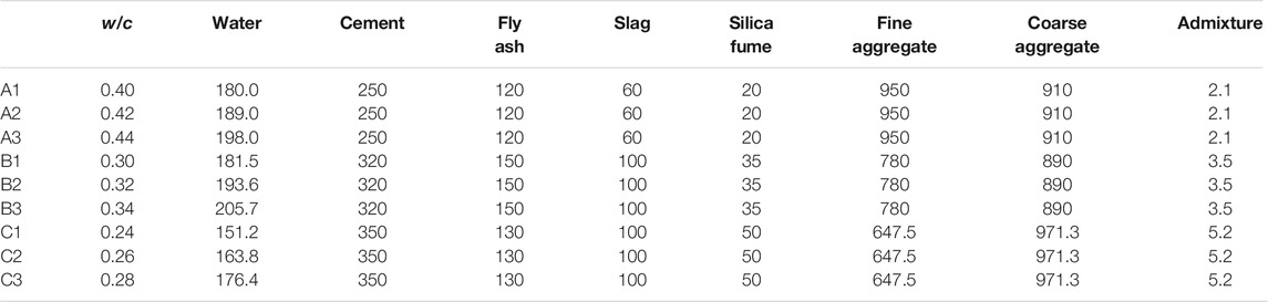
TABLE 1. Mixture proportions of concrete (kg/m3).
The slump test of spherical aggregate concrete was carried out according to the standard GB/T 50,080-2016, and the lifting speed of the slump cone was 0.06 m/s. A camera was arranged right above the slump cone to record the change of concrete slump flow with time, and the recording time interval was 0.05s. The slump test was repeated three times for each mix proportion, and the average value was taken as the test value of the slump and slump flow of spherical aggregate concrete. The slump and slump flow of A1 were 210 and 464 mm; the slump and slump flow of A2 were 227 and 506 mm; the slump and slump flow of A3 were 231 and 552 mm; the slump and slump flow of B1 were 201 and 449 mm; the slump and slump flow of B2 were 211 and 486 mm; the slump and slump flow of B3 were 226 and 517 mm; the slump and slump flow of C1 were 197 and 437 mm; the slump and slump flow of C2 were 209 and 469 mm; the slump and slump flow of C3 were 201 and 501 mm.
In this paper, the spherical aggregate concrete J-Ring test was conducted to investigate the passing ability of the concrete according to the standard GB/T 50,080-2016, and the lifting speed of the slump cone was 0.06 m/s. The J-Ring test was repeated three times for each mix proportion, and the average value was taken as the J-Ring slump-flow test value of spherical aggregate concrete. The J-Ring slump flow of A1, A2, A3, B1, B2, B3, C1, C2, and C3 was 448, 489, 534, 432, 471, 501, 422, 451, and 485 mm, respectively.
The V-funnel tests were conducted according to the standard GB/T 50,080-2016. The outflow time (TV) of concrete in V-funnel was recorded. The value of TV can reflect the viscosity and segregation resistance of concrete. The smaller the TV value, the smaller the plastic viscosity of concrete and the better the segregation resistance of concrete. The TV of A1, A2, A3, B1, B2, B3, C1, C2, and C3 was 5.5, 5.3, 5.1, 6.5, 6.3, 6.0, 7.3, 7.1, and 6.9 s, respectively.
The U-channel test was used to measure the filling height (Bh) of concrete. Bh can reflect the filling ability of concrete; that is, the smaller the Bh, the better the filling ability of concrete. The test was carried out according to the standard GB/T 50,080-2016. In the U-channel test, the lifting speed of the gate was 0.08 m/s. The test value of Bh of A1, A2, A3, B1, B2, B3, C1, C2, and C3 was 263, 264, 266, 250, 253, 255, 237, 239, and 241 mm, respectively.
The coefficient of restitution (e) reflected the degree of conservation of kinetic energy after collision between particle and geometry or between particle and particle in DEM. The value depended on the material, shape, collision direction, or collision speed that made up the collision element. The value of the coefficient of restitution was calculated from the relationship between the kinetic energy of the particle after the collision and the kinetic energy of the particle before the collision. According to González-Montellano et al. (2012), when the particles in the collision were not affected by rotation, the coefficient of restitution (for any type of collision) can be calculated using Eq. 1. The collision test to measure the coefficient of restitution is shown in Figure 1.
where u1 is the characteristic velocity before collision of free-falling particle; v1 is the characteristic velocity after collision of particle; u2 is the characteristic velocity before collision of the geometry; v2 is the characteristic velocity after collision of the geometry.
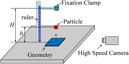
FIGURE 1. Test device for restitution coefficient.
In this paper, the meso-calibration test of particle-geometry restitution coefficient (eg) was similar to that of Gabriel KP Barrios (Barrios et al., 2013). The device allowed controllable collision between free-falling particles and the geometry plate, as shown in Figure 1. The particle was released from a fixed height H, falling freely and colliding with the geometry plate, and then bouncing to the height of h (lower than H). The free-fall height H and the bounce height h were determined using images taken by an i-SPEED 716 high-speed camera (Ix-camera, United Kingdom) at a rate of 100 frames per second.
The velocity v2 and u2 (Eq. 1) corresponding to the stationary geometry plate were taken as zero, and it was assumed that the energy was conserved before and after the collision. Therefore, the value of particle-geometry restitution coefficient can be expressed as a function of particle initial height H and bounce height h in Eq. 2:
In this paper, the concrete was regarded as composed of particles of aggregate wrapped by paste. In the particle-geometry restitution coefficient test, the free-falling particle was a glass sphere wrapped by paste (the composition of the paste was the same as that in the concrete), and the geometry plate was a stainless steel plate with the same material as the slump plate.
If the particle collision particle was directly used to measure the particle-particle restitution coefficient (ep), there were strict requirements on the collision angle between particles. Grima (2011) accurately measured particle-particle restitution coefficient by using a plate of the same material as the particle instead of the collided particle. In this paper, the glass plate with the same material and process as the glass particle was used instead of the collided particle. The geometry plate in Figure 1 was replaced with the glass plate for the particle-particle restitution coefficient test. The particle-particle restitution coefficient test procedure and device were the same as the particle-geometry restitution coefficient test.
The spherical glass aggregate (wrapped with mortar) taken directly from the fresh concrete was used as free-falling particle for the restitution coefficient test. The particles fell freely from four different fixed heights of 100, 90, 80, and 70 mm and collided with the geometry plate or glass plate. The test was repeated 10 times for each fixed height to obtain the average bounce height h.
The coefficient of rolling friction (μr) was an index to measure the resistance of a rolling object. This value represented the relationship between the tangential force of the rolling bodies and the normal force that kept the rolling body in contact. Ai et al. (2011) conducted the inclined test to measure the rolling friction coefficient of particle.
The inclined test device used in this paper was made up of an inclined plate, a high-precision angle measuring instrument (accuracy of 0.01°), and a high-precision lifting platform (lifting speed of 0.008 m/s), as shown in Figure 2. When the particle-geometry rolling friction coefficient (μrg) was measured, the stainless steel geometry plate was used as the inclined plate for testing.
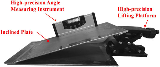
FIGURE 2. Inclined test device.
When testing the particle-geometry rolling friction coefficient, the particles were placed on the horizontal stainless steel inclined plate, and the handwheel of the lifting table was rotated to slowly raise the lifting table in order to increase the tilt angle of the stainless steel plate. When the particles rolled, a high-speed camera was recording the tilt angle of the inclined plate. The force condition of the particle on the stainless steel plate is shown in Figure 3.
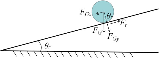
FIGURE 3. Balance of force in rolling friction test.
Equation 3 is the balance equation of the force of the particle on the inclined plate.
where Frg is the rolling friction force between the particle and the geometry inclined plate, in N; μrg is the rolling friction coefficient between the particle and the geometry inclined plate; FG is the gravity of the particle, in N; FGy is the normal component of gravity on the geometry inclined plate, and the unit is N; θrg is the angle between the geometry inclined plate and the horizontal plane, and the unit is °.
In the critical state where the particle was about to roll,
where FGx is the tangential component of gravity on the geometry inclined plate, and the unit is N; θrgc is the critical rolling angle of particle on the geometry inclined plate, and the unit is °.
Equation 4 was substituted into Eq. 3 to obtain
From Eq. 5, the value of particle-geometry rolling friction coefficient (μrg) was equal to the tangent value of the inclination angle when the particle was in the critical rolling state.
In the particle-particle rolling friction coefficient (μrp) test, the glass plate with the same material and production technology as the particle was used as the inclined plate to measure the particle-particle rolling friction coefficient (Grima, 2011). The test procedure and method were the same as the particle-geometry rolling friction coefficient.
The spherical glass aggregate (wrapped with mortar) taken directly from the fresh concrete was used as rolling particle for the rolling friction coefficient test. The test was conducted using glass spheres with particle sizes of 10, 9, 8, and 7 mm. The particle-geometry rolling friction coefficient test and particle-particle rolling friction coefficient test of each particle size were repeated 10 times to obtain the average critical rolling angle.
The coefficient of static friction (μs) was the ratio of the maximum static friction force to the normal force between the contact surfaces, calculated by measuring the critical slide angle when the concrete particles began to slide through the inclined test. The operation and procedure of the static friction coefficient inclined test were the same as the rolling friction coefficient inclined test.
Before testing the particle-geometry static friction coefficient (μsg), in order to avoid the particles rolling on the inclined plate, three particles with the same particle size were bonded together (Grima, 2011). This can effectively prevent the particles from rolling, before sliding occurred, and did not affect the calculation of the static friction coefficient of the particles, as shown in Figure 4.
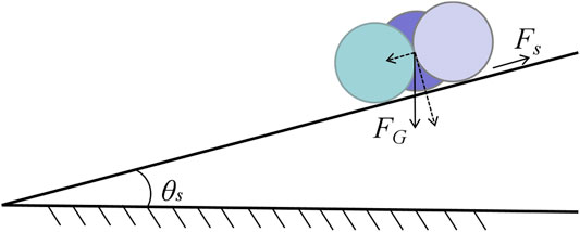
FIGURE 4. Balance of force in static friction test.
The balance equation of the force of the particles on the inclined plate was
where Fsg is the static friction force between the particle and the geometry inclined plate, in N; μsg is the static friction coefficient between the particle and the geometry inclined plate; θsg is the angle between the geometry inclined plate and the horizontal plane, in °. When the particles were in a sliding critical state,
where θsgc is the critical sliding angle of particles on the geometry inclined plate, in °. Equation 7 was substituted into Eq. 6 to calculate the particle-geometry static friction coefficient (μsg):
It can be seen from Eq. 8 that the value of particle-geometry static friction coefficient (μsg) was equal to the tangent value of critical sliding angle (θsgc).
The spherical glass aggregate (wrapped with mortar) taken directly from the fresh concrete was used as slipping particle for the static friction coefficient test. In the particle-particle static friction coefficient (μsp) test, the glass plate with the same material and production technology as the particle was used as the inclined plate to measure the particle-particle static friction coefficient (Grima, 2011). The test procedure and method were the same as the particle-geometry static friction coefficient.
The surface energy (γ) affected the adhesion of fresh concrete particles (Zafar et al., 2014). The surface energy value of fresh concrete particles was determined by the surface tension and wetting angle of the paste. In this paper, the pullout force between fresh concrete particles was measured by inclined test, and then the value of surface energy was calculated according to Eq. 9. In the incline test to measure the surface energy of JKR, the surface of the glass sphere was smooth, and the paste was only daubed on the contact position between the two particles, as shown in Figure 5. Particle A was fixed on the inclined plate. The tilting angle of the inclined plate increased evenly by adjusting the lifting table. When the inclined plate reached a certain angle, particle B began to get rid of the adhesion of the paste under the influence of gravity and rolled down. A high-speed camera was used to record the tilt angle of the inclined plate when the two particles separated.
where Fpullout is the pullout force exerted on particle B by the paste between the particles, in N; γ is the surface energy of the slurry, in J/m2; R* is the equivalent radius of particle A and particle B, in J/m2.
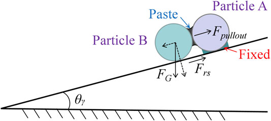
FIGURE 5. Balance of force in Fpullout test.
The force of particle B on the inclined plate is shown in Figure 5. The equilibrium equation of force for particle B was as follows:
where Frs is the rolling friction force between particle B and the inclined plate, in N; θγ is the angle between the inclined plate and the horizontal plane, in °.
The critical rolling angle (θγc) of particle B was larger than that of smooth particle when there was adhesion force between particles. When the inclination angle of particle B was larger than θrsc of smooth particle, the rolling friction force of particle B was
where μrs is the rolling friction coefficient of smooth glass particles and inclined plate. When particle B was in rolling critical state, Eq. 11 was substituted into Eq. 10, and Fpullout was calculated as follows:
Therefore, before calculating Fpullout, the rolling friction coefficient between the smooth glass particles and the inclined plate needed to be tested. This paper used the method of measuring the rolling friction coefficient of fresh concrete particles in “Coefficient of Rolling Friction” section to measure the critical rolling angle (θrsc) of the smooth glass particles and the inclined plate, and then μrs was calculated using Eq. 5.
This paper used 10, 9, 8, and 7 mm glass spheres for surface energy test. The surface energy test for each particle size was repeated 10 times to obtain the average separation angle between particles.
Before measuring Fpullout of the paste, the rolling friction coefficient of the smooth particles and the inclined plate was tested. After determining the rolling friction coefficient of the smooth glass particles and the inclined plate, the inclined test in Figure 5 was conducted to measure the critical rolling angle (θγc) of particles B when there was paste between the particles. Then, Eq. 12 was utilized to calculate Fpullout of the paste between the particles, and Eq. 9 was adopted to calculate the surface energy γ between the particles.
The Hertz–Mindlin with JKR (Johnson–Kendall–Roberts) cohesion (Kendall, 1971) was a cohesive force contact model, which considered the influence of cohesion in the particle contact area and mainly was used for discrete element simulation of particles with Van der Waals forces or wet particles. At present, the theoretical research of JKR model has been mature, and the physical meaning of contact parameters has been clear. In addition, the contact parameters of JKR model can be directly measured by test. In this paper, Hertz–Mindlin with JKR cohesion was used as the contact model of the concrete particles. Hertz–Mindlin with JKR model was an improvement of normal force based on Hertz–Mindlin (no slip) contact mode. In JKR model, the normal elastic contact force was realized based on JKR theory (Kendall, 1971). The tangential force of Hertz–Mindlin with JKR model was the same as that of Hertz–Mindlin (no slip) contact model.
The normal force component of the Hertz–Mindlin (no slip) model was calculated based on the Hertz contact theory (Hertz, 1880). The tangential force model was calculated based on the research results of Mindlin and Deresiewicz (Mindlin, 1949; Deresiewicz, 1953). The tangential friction followed the Coulomb friction law and was limited by μsFn. Both the normal force and the tangential force had damping components, and the damping coefficient was related to the restitution coefficient (Tsuji et al., 1992).
The normal force Fn was a function of the normal overlap δn between particles, calculated by Eq. 13:
where the equivalent Young’s modulus E* and equivalent radius R* were defined as
where Ei, νi, Ri and Ej, νj, Rj are Young’s moduli, Poisson’s ratios, and radiuses of particle i and particle j.
Normal damping force Fnd is calculated as follows:
where
where e is the coefficient of restitution.
The tangential force Ft depended on the tangential overlap δt and the tangential stiffness St, as follows:
where G* is the equivalent shear modulus.
Tangential damping force Ftd is calculated as follows:
where
The rolling friction torque was proportional to the normal contact force, and its direction was opposite to the relative rotation direction (Zhou et al., 1999). The rolling friction of the particles was performed by applying torque to the contact surface.
where μr is the rolling friction coefficient, Ri is the distance from the contact point to the center of mass, and ωi is the unit angular velocity vector of the object at the contact point.
The normal force of Hertz–Mindlin with JKR cohesion model increased a kind of cohesion on the basis of Hertz–Mindlin (no slip) normal force. The normal force FJKR of JKR model depended on the amount of overlap δ between particles and surface energy γ.
where a is the radius of the circular contact area formed between particles.
When γ = 0, the normal force of the JKR model was equal to the normal force of Hertz–Mindlin (no slip).
The JKR model can still provide the cohesive force when the particles were not in direct contact. The maximum gap δc and critical contact radius αc of non-zero cohesive force between particles were calculated by the following Eqs. 26, 27:
The maximum cohesion force occurred when the particles were not in contact and the separation gap was less than δc. This maximum cohesion force was called Fpullout, calculated by Eq. 9.
The restitution coefficient test results of B1 concrete are shown in Table 2. After the particles fell freely from different heights and collided with the geometry, the rebound height h decreased as the initial height H decreased. The restitution coefficients of different fixed heights were basically the same, and the average value of particle-geometry restitution coefficient (eg) was 0.248. The particle-particle collision test results were similar to the particle-geometry test results, and the average particle-particle restitution coefficient (ep) was 0.249.
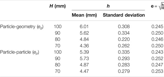
TABLE 2. The restitution coefficient test results of B1 concrete.
According to the test results of restitution coefficient of concrete particles with different mix proportions, the average restitution coefficients of nine concrete particles were calculated. The eg of nine concrete particles was 0.249, 0.254, 0.255, 0.248, 0.252, 0.254, 0.244, 0.250, and 0.253, respectively. The ep of nine concrete particles was 0.251, 0.255, 0.257, 0.249, 0.253, 0.256, 0.246, 0.251, and 0.255, respectively. The restitution coefficient of the three groups of concrete particles A, B, and C decreased with the increasing of the water-binder ratio.
The rolling friction coefficient test results of B1 concrete are shown in Table 3. The critical rolling angles (θrc) of particle-geometry of different particle sizes were similar, and the average value of particle-geometry rolling friction coefficient (μrg) was 0.107. The critical rolling angles (θrc) of particle-particle of different particle sizes were basically the same, and the average value of particle-particle rolling friction coefficient (μrp) was 0.090.
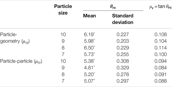
TABLE 3. The rolling friction coefficient test results of B1 concrete.
The average rolling friction coefficients (μrg) of the concrete particles of the nine mix ratios were 0.104, 0.094, 0.090, 0.106, 0.102, 0.095, 0.113, 0.101, and 0.097, respectively. The average rolling friction coefficients (μrp) of the concrete particles of the nine mix ratios were 0.083, 0.073, 0.071, 0.086, 0.083, 0.080, 0.104, 0.081, and 0.079, respectively. The particle-geometry rolling friction coefficient and particle-particle rolling friction coefficient values of the three groups of concrete of A, B, and C decreased with the increase of the water-binder ratio.
The static friction coefficient test results of B1 concrete are shown in Table 4. The critical slide angles (θsc) of particle-geometry of different particle sizes were close, and the average value of particle-geometry static friction coefficient (μsg) was 0.228. The critical slide angles (θsc) of particle-particle of different particle sizes were about the same, and the average value of particle-particle static friction coefficient (μsp) was 0.192.
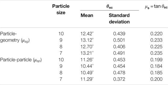
TABLE 4. The static friction coefficient test results of B1 concrete.
The average particle-geometry static friction coefficients (μsg) of nine concrete particles were 0.221, 0.201, 0.188, 0.228, 0.206, 0.196, 0.233, 0.225, and 0.204, respectively. The average particle-particle static friction coefficients (μsp) of nine concrete particles were 0.190, 0.184, 0.182, 0.192, 0.185, 0.174, 0.223, 0.191, and 0.186, respectively. The values of static friction coefficient of concrete in groups A, B, and C decreased with the increase of water-binder ratio.
The test results of rolling friction coefficient of glass sphere are shown in Table 5. The critical rolling angle (θrs) between the four smooth particles and the inclined plate was basically close, and the average rolling friction coefficient was 0.018.
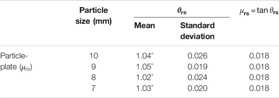
TABLE 5. The test results of rolling friction coefficient of smooth glass particles.
After determining the rolling friction coefficient between the smooth particles and the inclined plate, the critical rolling angle (θγc) of particle B was measured using the tilt test of Figure 5, and then Fpullout and surface energy (γ) of the paste between the particles were calculated. The test results of surface energy of B1 concrete are shown in Table 6. The surface energy of the paste between particles of different sizes was basically the same, and the average surface energy γ was 0.370 J/m2. As the particle size decreased, the critical separation angle (θγc) of particle B increased. The reason was that when the gravity of particle B decreased, a larger separation angle was needed to increase the tangential force of particle B on the inclined plate to get rid of Fpullout of the paste.
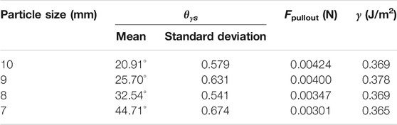
TABLE 6. The surface energy test results of B1 concrete.
According to the surface energy test results of concrete particles with different mix proportions, the average surface energy of paste in the nine types of concrete mix proportions were calculated. The surface energy (γ) of the nine concrete particles was 0.368, 0.364, 0.363, 0.370, 0.366, 0.361, 0.373, 0.368, and 0.364 J/m2, respectively. The surface energy of the three groups of concrete particles decreased with the increase of the water-binder ratio.
The amount of cementitious material and water-binder ratio are the main factors affecting the contact parameters of concrete particles. With the change of the composition and amount of cementitious materials, the viscosity of the paste on the surface of concrete particles also changed. When the viscosity of paste increased, the restitution coefficient of concrete particles decreased, and the static friction coefficient, rolling friction coefficient, and surface energy increased.
The slump test model was established according to the actual size of the slump cone and slump plate, and then the intrinsic parameters (density, shear modulus, and Poisson's ratio) of the geometry (slump cone and slump plate) were defined. The material of the test equipment used in the slump test and calibration test was stainless steel, the density was 7,750 kg/m3, the shear modulus was 72.797 GPa, and Poisson's ratio was 0.305.
This paper used EDEM software to establish a single-phase element concrete DEM model (Hoornahad and Koenders, 2014). The concrete was considered to be composed of mortar-wrapped glass aggregate particles. The intrinsic parameters of the particles were defined according to the aggregate density, shear modulus, and Poisson's ratio in “Aggregate” section. Then, the test results of restitution coefficient, rolling friction coefficient, static friction coefficient, and surface energy were used as the contact parameters of particle-geometry and particle-particle in the concrete DEM model to simulate. Finally, the concrete particles were generated in the slump cone. Before generating the concrete particles, a funnel was added above the slump cone to increase the rate of particle generation. After the particles filled the slump cone, the funnel and excess particles above the slump cone were removed. The establishment of the DEM model of concrete slump test was finished.
The J-Ring model was added to the DEM model of the slump test to investigate the passing ability of concrete. The J-Ring test DEM model was established based on the J-Ring size recommended by the standard GB/T 50,080-2016. The material of J-Ring was the same as that of the slump test.
The V-funnel model and U-channel model were established based on the size recommended by the standard GB/T 50,080-2016. The materials of V-funnel and U-channel were the same as that of the slump test.
The slump cone in the DEM model was lifted off at a speed of 0.06 m/s to simulate the concrete slump test. The results of the slump test and the DEM model of B1 concrete at 0.9 and 4 s are shown in Figures 6A,B. At 0.9 s, the test value of the slump flow was 302 mm, and the slump flow and slump of the DEM model were 303 and 178 mm, respectively. At 4 s, the test values of the slump flow and slump were 449 and 201 mm, the slump flow and slump of the DEM model were 407 and 203 mm, and the relative deviations were 0.445 and 0.995%, respectively. The simulation results of B1 concrete DEM model at 0.9 and 4 s were in good agreement with the test results.
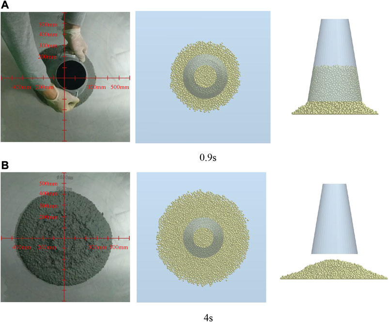
FIGURE 6. Comparison between slump test process and DEM simulation of B1 concrete: (A) 0.9 s and (B) 4 s.
The changes in the slump flow of the DEM model and the test over time were recorded, and the slump flow–time curve is shown in Figure 7. The slump flow–time curves of test and DEM model can be divided into three stages. Stage I was the initial stage. When the slump cone began to lift off, the lift-off distance between the bottom of slump cone and the slump plate was small, and the large-size aggregates in concrete were hindered by the bottom of slump cone, which limited the flow of concrete. Stage II was the rapid flow stage. The gravity potential energy of concrete in slump cone was rapidly converted into kinetic energy, and the concrete flowed rapidly under the action of gravity. Stage III was the slow flow stage. After the gravity potential energy of concrete decreased, the kinetic energy of concrete was gradually consumed by the friction force of slump plate, and the flow velocity of concrete decreased and finally tended to be static. In these three stages, the slump flow–time curve simulated by DEM was in good agreement with the test results.
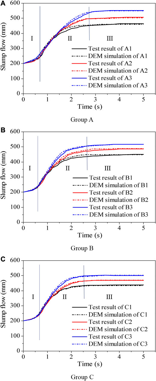
FIGURE 7. Comparison of test and simulation by slump flow–time curves: (A) Group A, (B) Group B, and (C) Group C.
The relative deviation of slump simulation of nine types of concrete was 0.952, 0.881, 1.299, 0.995, 0.474, 0.442, 1.015, 0.478, and 0.459%, respectively. The relative deviation of slump-flow simulation of the nine concrete types was 0.647, 0.791, 0.362, 0.445, 0.412, 0.193, 0.686, 0.213, and 0.399%, respectively. The relative deviations between the slump and slump-flow simulation results of the concrete DEM model and the test results were very small. The average relative deviation between the slump simulation value and the test value of nine types of concrete was 0.777%, and the average relative deviation between the slump-flow simulation value and the test value was 0.461%. The DEM contact model and calibrated contact parameters used in this paper can accurately simulate the process and results of concrete slump test.
The slump cone was lifted up at a speed of 0.06 m/s. The J-Ring DEM simulation of B1 concrete is shown in Figure 8. The J-Ring slump flow of the concrete DEM model was 297 mm at 0.9 s and 431 mm at 4 s. The simulation results of DEM model were close to the test results of concrete J-Ring slump flow. The difference between the slump flow of concrete and the J-Ring slump flow was used as the performance index of the passing ability. The DEM simulation results of J-Ring slump flow were 446, 487, 532, 431, 472, 499, 418, 453, and 486 mm, and the relative deviation was 0.446, 0.409, 0.375, 0.231, 0.212, 0.399, 0.948, 0.444, and 0.206%, respectively. The passing ability of nine types of concrete was 15, 15, 18, 16, 16, 17, 16, 17, and 17 mm, and the relative deviation was 6.25, 11.76, 0.00, 5.88, 6.67, 6.25, 6.67, 5.56, and 6.25%, respectively. The simulation results of J-Ring slump flow and passing ability of concrete DEM model were similar to the test results. The average relative deviation between the J-Ring slump-flow simulation value and the test value of nine types of concrete was 0.408%, and the average relative deviation between the passing ability simulation value and the test value was 6.14%. The concrete DEM model established in this paper can simulate the passing ability of concrete well.
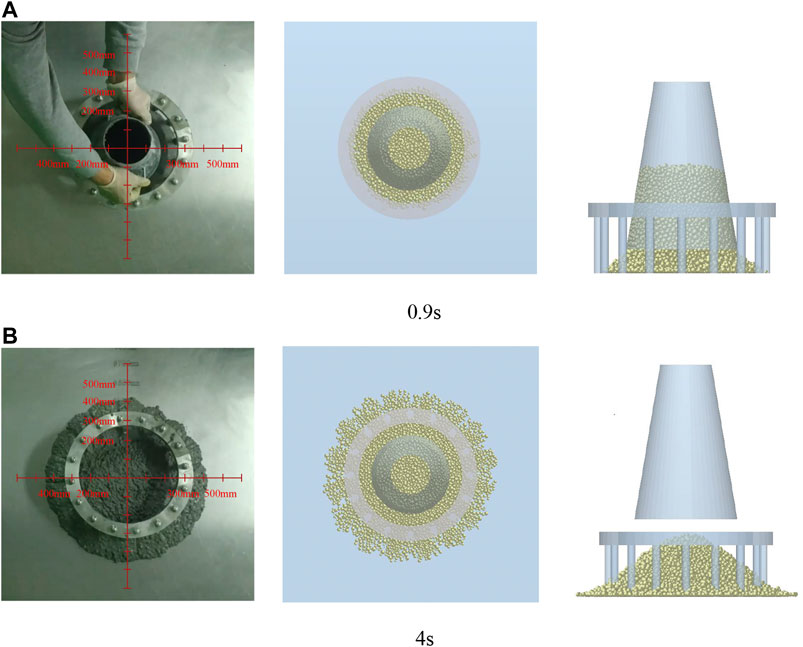
FIGURE 8. Comparison between J-Ring test process and DEM simulation of B1 concrete: (A) 0.9 s and (B) 4 s.
The velocity distribution of B1 concrete in V-funnel is shown in Figure 9A. At the beginning of flow, the flow velocity at the outlet was maximum, the flow velocity of concrete particles above the outlet decreased gradually, and the flow velocity of concrete particles above the funnel was close to zero. Above the outlet of V-funnel, the velocity distribution of concrete particles at different outflow time was basically similar, and the velocity distribution near the outlet was almost not affected by the flow time. The simulation values of TV of A1, A2, A3, B1, B2, B3, C1, C2, and C3 were 5.4, 5.3, 5.2, 6.4, 6.2, 6.1, 7.1, 6.8, and 6.6 s, respectively. The relative deviation of V-funnel simulation of the nine types of concrete was 1.82, 0.00, 1.96, 1.54, 1.59, 1.67, 2.74, 4.2, and 4.35%, respectively, and the average relative deviation was 2.21%. With the increase of water-cement ratio, the viscosity of concrete decreased, which led to the decrease of TV.
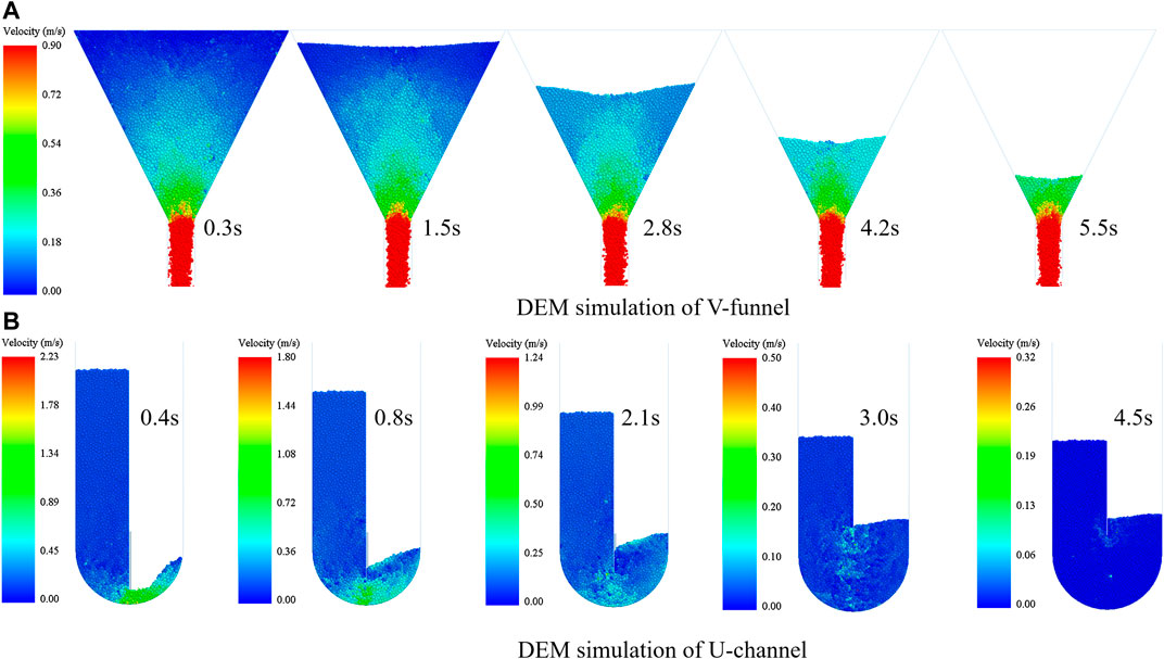
FIGURE 9. Simulation of V-funnel and U-channel: (A) DEM simulation of V-funnel and (B) DEM simulation of U-channel.
The velocity distribution of B1 concrete in U-channel is shown in Figure 9B. The gate was lifted at a speed of 0.08 m/s, and the concrete flowed quickly to the right side. The concrete particles in the left side of U-channel flowed down uniformly and slowly. With the increase of flow time, the maximum flow velocity of concrete gradually decreased, and the velocity distribution of concrete changed greatly. The maximum flow velocity occurred below the gate, and the position of the maximum flow velocity moved up with the lifting of the gate. After 4.5 s, the concrete gradually tended to static state. The simulation values of Bh of A1, A2, A3, B1, B2, B3, C1, C2, and C3 were 261, 262, 264, 248, 251, 252, 235, 236, and 238 mm, respectively. The average relative deviation of the simulation result was 0.931%. The simulation results were in good agreement with the test results.
In the simulation of concrete fluidity, the static friction coefficient had the greatest influence on the simulation results, followed by the rolling friction coefficient, and the restitution coefficient had the least influence on the simulation results. Therefore, it is necessary to accurately measure the contact parameters of concrete particles, and the contact parameters of concrete particles measured by tests are closer to the real results than the trial-error method.
In this paper, high-precision glass spheres were used as aggregates for the slump test and meso-calibration test of fresh concrete. Through a series of meso-calibration tests, the contact parameters of the discrete element model of fresh concrete were accurately measured, and the reliability of the DEM model was verified by the slump test. Through meso-calibration tests and DEM model verification, the following conclusions are obtained:
(1) The contact parameters of JKR contact model, such as coefficient of restitution, coefficient of rolling friction, coefficient of static friction, and surface energy, can be measured accurately by collision test and inclined test.
(2) It is feasible to use glass sphere instead of concrete aggregate for parameter measure of DEM model.
(3) The DEM model established by the JKR model and contact parameter calibration method can accurately simulate the flowability of concrete.
In this paper, spherical aggregate was used instead of gravel in concrete fluidity test and calibration test, which verified the reliability of meso-calibration test. In the following work, the author will use the actual aggregate to carry out systematic calibration tests to measure the contact parameters of the real aggregate.
The original contributions presented in the study are included in the article/Supplementary Material. Further inquiries can be directed to the corresponding author.
YL contributed to the conception and research method of the study. JH was responsible for testing and organizing the database. ZW performed the statistical analysis. JL and CJ wrote the first draft of the manuscript. All authors contributed to manuscript revision and read and approved the submitted version.
The authors would like to acknowledge the financial support by the National Key R&D Program of China-Key materials and preparation technology of high crack resistant ready-mixed concrete (2017YFB0310100), National Natural Science Foundation of China (51808015) and General project of science and technology plan of Beijing Municipal Commission of Education (KM202110005018).
The authors declare that the research was conducted in the absence of any commercial or financial relationships that could be construed as a potential conflict of interest.
Ai, J., Chen, J.-F., Rotter, J. M., and Ooi, J. Y. (2011). Assessment of rolling resistance models in discrete element simulations. Powder Technol. 206 (3), 269–282. doi:10.1016/j.powtec.2010.09.030
Barrios, G. K. P., de Carvalho, R. M., Kwade, A., and Tavares, L. M. (2013). Contact parameter estimation for DEM simulation of iron ore pellet handling. Powder Technol. 248, 84–93. doi:10.1016/j.powtec.2013.01.063
Cao, G., Zhang, H., Tan, Y., Wang, J., Deng, R., Xiao, X., et al. (2015). Study on the effect of coarse aggregate volume fraction on the flow behavior of fresh concrete via DEM. Procedia Eng. 102, 1820–1826. doi:10.1016/j.proeng.2015.01.319
Coetzee, C. J. (2016). Calibration of the discrete element method and the effect of particle shape. Powder Technol. 297, 50–70. doi:10.1016/j.powtec.2016.04.003
Coetzee, C. J. (2017). Review: calibration of the discrete element method. Powder Technol. 310, 104–142. doi:10.1016/j.powtec.2017.01.015
Chinese Standard (2002). Chinese Standard GB/T 50081-2002, Standard for test method of mechanical properties on ordinary concrete. China: Ministry of Construction of the People's Republic of China. [in Chinese].
Cui, W., Ji, T., Li, M., and Wu, X. (2016). Simulating the workability of fresh self-compacting concrete with random polyhedron aggregate based on DEM. Mater. Struct. 50 (1), 1–12. doi:10.1617/s11527-016-0963-9
Cui, W., Yan, W.-s., Song, H.-f., and Wu, X.-l. (2018). Blocking analysis of fresh self-compacting concrete based on the DEM. Construct. Build. Mater. 168, 412–421. doi:10.1016/j.conbuildmat.2018.02.078
Deresiewicz, H. (1953). Elastic spheres in contact under varying oblique forces. J. Appl. Mech. 20 (3), 327–344. doi:10.1007/978-1-4613-8865-4_35
González-Montellano, C., Fuentes, J. M., Ayuga-Téllez, E., and Ayuga, F. (2012). Determination of the mechanical properties of maize grains and olives required for use in DEM simulations. J. Food Eng. 111 (4), 553–562. doi:10.1016/j.jfoodeng.2012.03.017
Grima, A. P. (2011). Quantifying and modelling mechanisms of flow in cohesionless and cohesive granular materials. Wollongong, NSW: University of Wollongong.
Guo, Z.-Q., Yuan, Q., Stroeven, P., Fraaij, A. L. A., Lu, J. W. Z., Leung, A. Y. T., et al. (2010). Discrete element method simulating workability of fresh concrete. AIP Conf. Proc. 14, 430–435. doi:10.1063/1.3452210
Hertz, H. (1880). On the contact of elastic solids. J. für die Reine Angewandte Math. (Crelle's J.). 92, 156–171.
Hoornahad, H., and Koenders, E. A. B. (2014). Simulating macroscopic behavior of self-compacting mixtures with DEM. Cement Concr. Compos. 54, 80–88. doi:10.1016/j.cemconcomp.2014.04.006
Hou, D., Lu, Z., Li, X., Ma, H., and Li, Z. (2017). Reactive molecular dynamics and experimental study of graphene cement composites: structure, dynamics and reinforcement mechanisms. Carbon 115, 188–208.
Krenzer, K., Mechtcherine, V., and Palzer, U. (2019). Simulating mixing processes of fresh concrete using the discrete element method (DEM) under consideration of water addition and changes in moisture distribution. Cement Concr. Res. 115, 274–282. doi:10.1016/j.cemconres.2018.05.012
Kendall, K. (1971). Surface energy and the contact of elastic solids. Proc. Math. Phys. Eng. Sci. 324 (1558), 301–313. doi:10.1098/rspa.1971.0141
Li, Z., Cao, G., and Guo, K. (2018). Numerical method for thixotropic behavior of fresh concrete. Construct. Build. Mater. 187, 931–941. doi:10.1016/j.conbuildmat.2018.07.201
Mechtcherine, V., Gram, A., Krenzer, K., Schwabe, J.-H., Shyshko, S., and Roussel, N. (2013). Simulation of fresh concrete flow using Discrete Element Method (DEM): theory and applications. Mater. Struct. 47 (4), 615–630. doi:10.1617/s11527-013-0084-7
Mechtcherine, V., and Shyshko, S. (2015). Simulating the behaviour of fresh concrete with the Distinct Element Method—deriving model parameters related to the yield stress. Cement Concr. Compos. 55, 81–90. doi:10.1016/j.cemconcomp.2014.08.004
Mindlin, R. D. (1989). Compliance of elastic bodies in contact. J. Appl. Mech. 16, 197–268. doi:10.1007/978-1-4613-8865-4_24
Pieralisi, R., Cavalaro, S. H. P., and Aguado, A. (2016). Discrete element modelling of the fresh state behavior of pervious concrete. Cement Concr. Res. 90, 6–18. doi:10.1016/j.cemconres.2016.09.010
Rackl, M., and Hanley, K. J. (2017). A methodical calibration procedure for discrete element models. Powder Technol. 307, 73–83. doi:10.1016/j.powtec.2016.11.048
Remond, S., and Pizette, P. (2014). A DEM hard-core soft-shell model for the simulation of concrete flow. Cement Concr. Res. 58, 169–178. doi:10.1016/j.cemconres.2014.01.022
Shyshko, S., and Mechtcherine, V. (2013). Developing a Discrete Element Model for simulating fresh concrete: experimental investigation and modelling of interactions between discrete aggregate particles with fine mortar between them. Construct. Build. Mater. 47, 601–615. doi:10.1016/j.conbuildmat.2013.05.071
Shyshko, S., and Mechtcherine, V. (2008). “Simulating the workability of fresh concrete,” in International RILEM Symposium on Concrete Modelling, 173–181.
Tan, Y., Cao, G., Zhang, H., Wang, J., Deng, R., Xiao, X., et al. (2015). Study on the thixotropy of the fresh concrete using DEM. Procedia Eng. 102, 1944–1950. doi:10.1016/j.proeng.2015.06.138
Tsuji, Y., Tanaka, T., and Ishida, T. (1992). Lagrangian numerical simulation of plug flow of cohesionless particles in a horizontal pipe. Powder Technol. 71 (3), 239–250. doi:10.1016/0032-5910(92)88030-L
Zafar, U., Hare, C., Hassanpour, A., and Ghadiri, M. (2014). Drop test: a new method to measure the particle adhesion force. Powder Technol. 264, 236–241. doi:10.1016/j.powtec.2014.04.022
Zhan, Y., Gong, J., Huang, Y., Shi, C., Zuo, Z., and Chen, Y. (2019). Numerical study on concrete pumping behavior via local flow simulation with discrete element method. Materials 12 (9), 1415–1435. doi:10.3390/ma12091415
Zhang, X., Zhang, Z., Li, Z., Li, Y., and Sun, T. (2020). Filling capacity analysis of self-compacting concrete in rock-filled concrete based on DEM. Construct. Build. Mater. 233, 117321. doi:10.1016/j.conbuildmat.2019.117321
Zhao, Y., Han, Z., Ma, Y., and Zhang, Q. (2018). Establishment and verification of a contact model of flowing fresh concrete. Eng. Comput. 35 (7), 2589–2611. doi:10.1108/ec-11-2017-0447
Keywords: discrete element method, meso-calibration test, contact parameter, Hertz–Mindlin with JKR, concrete flowability, passing ability
Citation: Li Y, Hao J, Jin C, Wang Z and Liu J (2021) Simulation of the Flowability of Fresh Concrete by Discrete Element Method. Front. Mater. 7:603154. doi: 10.3389/fmats.2020.603154
Received: 05 September 2020; Accepted: 28 December 2020;
Published: 08 February 2021.
Edited by:
Dongshuai Hou, Qingdao University of Technology, ChinaCopyright © 2021 Li, Hao, Jin, Wang and Liu. This is an open-access article distributed under the terms of the Creative Commons Attribution License (CC BY). The use, distribution or reproduction in other forums is permitted, provided the original author(s) and the copyright owner(s) are credited and that the original publication in this journal is cited, in accordance with accepted academic practice. No use, distribution or reproduction is permitted which does not comply with these terms.
*Correspondence: Zigeng Wang, emlnZW5nd0BianV0LmVkdS5jbg==
Disclaimer: All claims expressed in this article are solely those of the authors and do not necessarily represent those of their affiliated organizations, or those of the publisher, the editors and the reviewers. Any product that may be evaluated in this article or claim that may be made by its manufacturer is not guaranteed or endorsed by the publisher.
Research integrity at Frontiers
Learn more about the work of our research integrity team to safeguard the quality of each article we publish.