Exploring Adaptive Behavior of Non-linear Hexagonal Frameworks

Non-linear structural responses offer a rich design space that can be integrated into the development of novel (meta)-materials to enable transformative capabilities. By exploiting robust, repeatable, non-linear elasticity the (meta)-material's performance can be tailored to significantly exceed what has been demonstrated through traditional linear design paradigms. Embracing geometric non-linearity offers the designer the potential for truly bespoke large-range elastic behavior. Herein we explore the behavior of bistable elements that can be arranged into a space-filling triangular lattice, constructed in a hierarchical manner. We develop an analysis of the system that can be readily extended to more complex hierarchies, such as the hexagonal arrangement considered herein, whilst retaining physical insight. Specifically, we present the geometric restrictions of lattice elements that govern the existence of stable stress-free states and subsequently characterize the transitions between such states by searching for the minimum energetic transition pathway. Through our approach, we explore how hierarchical multi-stable systems can be analyzed, thus contributing to the development of truly bespoke adaptive (meta-)materials.

1. Introduction

Traditional structural design practice typically utilizes stiff components whose deformations are purposefully minimized in order to exploit linear elastic behavior. Where large deformations are required, such as in morphing or deployable systems, mechanical joints are typically used to achieve the desired transformative behavior. With the advent of new manufacturing capabilities and advanced analysis tools, a purely linear design philosophy is increasingly being challenged. One example of this paradigm shift is the development of compliant mechanisms that utilize reversible but large structural deformations to achieve adaptability, oftentimes facilitated by snapping across regions of static instability. Advantages of such compliant mechanisms are decreased part count, reduced design complexity and the introduction of preferable manufacturing techniques (Howell, 2001). Most importantly, in compliant systems the structural topology can be tailored to obtain desirable transformative behavior (see e.g.,Lu and Kota, 2003; Jutte and Kota, 2008; Krishnan et al., 2013).

Harnessing structural instabilities is not without its own challenges, see e.g.,Champneys et al. (2019) who outline recent advances in the field. One prominent example is the buckling of an axially compressed cylindrical shell, which, beyond the classical periodic buckling waveforms distributed over the entire domain of the cylinder, has a strong proclivity to localize the buckling mode over only a small portion of the domain, thereby forming localized dimples (Groh and Pirrera, 2019a). High-speed photography experiments of axially loaded cylinders suggest that a single dimple forms to initiate buckling, and this single dimple multiplies circumferentially to complete a single row of buckles (Eßlinger, 1970). This pattern formation, known as homoclinic snaking or cellular buckling, is also observed in numerical simulations (e.g., Hunt et al., 1999, 2000a; Groh and Pirrera, 2019a).

Owing to the rotational invariance of the cylinder, each unique combination of dimples can occur anywhere around the circumference, and the spatial multiplicity of these localizations implies a large set of possible trajectories to instability, with each trajectory affine to a particular imperfection signature (Groh and Pirrera, 2019b). The resulting complexity of multiple and oftentimes entangled post-buckling paths of this symmetric problem creates unique challenges for numerical methods, for the interpretation of results, and for obtaining physical insight into problem. However, the sequence of instabilities can be controlled more reliably by breaking the system's inherent symmetry through engineered imperfections (Lee et al., 2016) or through tailored material properties (White et al., 2015).

Similar difficulties are indeed also faced in the (meta)-material community that is developing novel material systems constructed from multi-scale arrangements of mechanically multi-stable snapping components (Mullin et al., 2007; Florijn et al., 2014; Nadkarni et al., 2014; Rafsanjani et al., 2015, 2019; Shan et al., 2015). As the periodicity of the unit cells is scaled-up, e.g., by placing multiple unit cells in rows and columns to create a 2D array, the complexity in the number of possible equilibrium states scales geometrically (Hunt and Dodwell, 2019). This is because under load many different deformation sequences can ensue; cells may snap individually, together as a row or column, or together as an entire array. The specific sequence of buckling is highly sensitive to the initial configuration of the system and thus presents close similarities to the cylinder buckling problem. The sequence of instabilities can thus be choreographed by introducing a bias into the system, either by varying the properties of individual unit cells or by adding initial imperfections (Che et al., 2016). These complexities often make obtaining physical insight into the behavior more difficult and the reliance on numerical methods can lead to computationally expensive design and optimization processes. Clearly, it is desirable to harness structural non-linearities in a manner that allows physical intuition to be retained and that permits an algorithmic approach to design. One approach to meeting this challenge is to exploit constrained non-linear behavior, which can be readily understood, to develop hierarchical systems. For example, the helical lattices investigated by Pirrera et al. (2013) may be thought of as well-understood 1D non-linear springs whose behavior is tuned by varying stiffness, pre-stress and characteristic lengths (a macroscopic example is shown in Figure 1). An extension to the analytical model of Pirrera et al. (2013) for lattices with strips of nominal width, thereby including their transverse curvature and in-plane strains, demonstrates a robust consistency with finite element simulation and experimental characterizations (McHale et al., 2020b). Furthermore, the helical lattice can be tuned to exploit external fields, such as thermal effects (O'Donnell et al., 2019; McHale et al., 2020a), to modulate the effective stiffness and stability landscape. The potential of helical lattices to obtain truly bespoke elastic responses was considered by Dixon et al. (2019). By exploiting the helical lattice as a structural base-unit for non-linear systems of coupled lattices, an algorithmic tuning process that can match, to an arbitrary precision, any energetic function up to a constant was developed (Dixon et al., 2019).

FIGURE 1

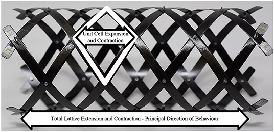
Figure 1. Prototype of a helical lattice structure that behaves as a one-dimensional non-linear spring. Figure reproduced from O'Donnell et al. (2019).

Emergent behavior is not restricted to the helical lattice alone and there exists a range of non-linear units from which emergent behavior is observed as system complexity is increased, such as cylindrical ribbons (Lachenal et al., 2012; Aza et al., 2019; Carey et al., 2019) and snapping arches (Hunt and Dodwell, 2019). This paper seeks to extend the design concepts explored in Dixon et al. (2019) beyond their current one-dimensional nature through an exploration of hierarchical space-filling lattices. In doing so, we take one step closer toward the design of truly bespoke (meta-)materials.

At smaller length-scales, the architecture of non-linear (meta-)materials can be informed by structural behavior, thereby reducing reliance on time-consuming and complex investigations based on material science—as is the case for tuning the properties of shape memory alloys (Bhattacharya and James, 2005). Instead, using a structural approach, instabilities can be integrated into the design and exploited to obtain a unique richness in system response (Reis, 2015; Bertoldi, 2017). By employing these structural response mechanisms at sufficiently small length scales, a desirable macroscopic continuum response can be achieved (O'Donnell et al., 2016; O'Donnell et al., 2019). Herein, we propose a new approach for creating novel material behavior from a hierarchy of non-linear elements; namely, rather than utilizing complex topologies to achieve the desired non-linear behavior, we can subsume this complexity into well understood non-linear “springs” acting as base-units of a hierarchical design. By combining robust base-units in simple lattices, in this case triangular lattices, we can achieve desirable morphing characteristics.

The paper proceeds as follows. First, we identify the base bistable element from which our lattices derive. Then we explore the stable stress-free configurations of a triangular framework, the so-called first hierarchy, and describe its transitional behavior. Finally, we extend the lattice to the second hierarchy, namely a hexagonal framework, and identify the geometric restrictions that dictate the existence of stable stress-free states. We then explore the least-energy transitions between these states.

2. One-Dimensional Bistable Elements

We seek to investigate the behavior of frameworks composed of one-dimensional bistable elements which are non-linear springs characterized by a non-dimensional length l ∈ ℝ⁺ and non-dimensional energy Π(l) ⩾ 0. We assume that the two stable equilibria, which have zero energy, occur at lengths l = l₀ ∈ (0.5, 1) and l = 1. We also assume that the unstable equilibrium at l_p ∈ (l₀, 1) has energy Π(l_p) = 1, which is thus the energy barrier Π_B between the stable equilibria.

The energy profile of such elements can be tuned by tailoring their characteristic properties and can even match a target energy profile with an arbitrary level of accuracy (Dixon et al., 2019). However for computational ease we choose $l_p=\frac{l_0+1}{2}$ and select Π to be a fourth-order polynomial

$\begin{array}{ll}\Pi (l)={\displaystyle \sum _{i=0}^4}{c}_i{l}^i& (\mathrm{1a})\end{array}$

with coefficients c_i that satisfy

$\begin{array}{ll}\left[\begin{array}{c}{c}_4\\ c_3\\ c_2\\ c_1\\ c_0\end{array}\right]={\left[\begin{array}{ccccc}1& 1& 1& 1& 1\\ l_0^4& l_0^3& l_0^2& l_0& 1\\ l_p^4& l_p^3& l_p^2& l_p& 1\\ 4& 3& 2& 1& 0\\ 4l_0^3& 3l_0^2& 2l_0& 1& 0\end{array}\right]}^{-1}\left[\begin{array}{c}0\\ 0\\ 1\\ 0\\ 0\end{array}\right].& (\mathrm{1b})\end{array}$

The resulting energy is illustrated in Figure 2.

FIGURE 2

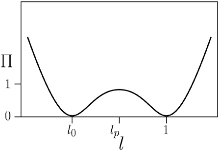
Figure 2. Energy function Equation (1) of a bistable element.

To characterize the zero-energy state of frameworks it is convenient to assign a “sign” to the elements of $\{l_0,1,\frac{1}{l_0}\}$ as follows:

$\begin{array}{ll}\text{sign }{l}_0:=-,\text{ sign }1:=0,\text{ sign }\frac{1}{l_0}:=+.& (2)\end{array}$

We will identify “+” with 1 and “−” with −1 so signs can be added and multiplied, see section 5 below.

3. Uncoupled Systems. I. Minima, Saddles and Maxima

Consider planar hinged structures, constructed from identical bistable elements, for which the element lengths can be prescribed independently of each other, restricted only by satisfaction of the triangle inequality, see Figure 3. (The two-element system in Figure 3A requires also specification of the fixed-support separation, L_sep.) We refer to such systems as uncoupled. Their energy is simply the sum of the energy of each element,

$\begin{array}{ll}{\Pi }^N(\text{l})={\displaystyle \sum _{n=1}^N}\Pi (l_n).& (3)\end{array}$

FIGURE 3

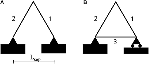
Figure 3. Examples of systems with (A) two elements and (B) three elements.

3.1. Triangles. I. Minima

In particular, the triangular structure in Figure 3B has 8 stable stress-free configurations, namely when its sides are of length either l₀ or 1. We label the (interior) angles of these configurations as follows. Consider a triangle with sides s₁, s₂, s₃ ∈ {l₀, 1}. We denote the angle subtended by the sides s₁, s₂ by a symbol chosen from {ϕ₀₋, ϕ₀₀, ϕ₀₊, ϕ_±−, ϕ_±+} as follows: The first subscript is 0 if s₁ = s₂ and is ± otherwise. The second subscript is 0 if s₁ = s₂ = s₃; else it is − if s₃ = l₀ and + if s₃ = 1.

From the cosine rule,

$\begin{array}{l}{\varphi }_{0-}=arccos(1-\frac{l_0^2}{2}),{\varphi }_{0+}=arccos(1-\frac{1}{2l_0^2}),\\ {\varphi }_{00}=arccos(\frac{1}{2})=\frac{\pi }{3},& (\mathrm{4a})\end{array}$

$\begin{array}{ll}{\varphi }_{\pm -}=arccos\frac{1}{2l_0},{\varphi }_{\pm +}=arccos\frac{l_0}{2}.& (\mathrm{4b})\end{array}$

Moreover, by considering the non-equilateral configurations we obtain,

$\begin{array}{ll}{\varphi }_{0-}+2{\varphi }_{\pm +}=\pi ,& (\mathrm{5a})\end{array}$

$\begin{array}{ll}{\varphi }_{0+}+2{\varphi }_{\pm -}=\pi ;& (\mathrm{5b})\end{array}$

and a simple calculation shows that the angles are ordered as.

$\begin{array}{ll}0<\left\{{\varphi }_{\pm -},{\varphi }_{0-}\right\}<\frac{\pi }{3}={\varphi }_{00}<{\varphi }_{\pm +}<{\varphi }_{0+}<\pi .& (6)\end{array}$

3.2. Triangles. II. Saddles and Maximum

Restricting the lengths of the elements to the interval [l₀, 1], we observe that local minima of the system energy correspond to configurations where all elements are at a local minimum of Π, i.e., of length either l₀ or 1. The system's only maximum occurs when all elements are at a local maximum of Π, i.e., of length l_p. Saddle points, i.e., extrema that are neither local maxima or minima (equivalently, where the Hessian is indefinite), correspond to configurations where some elements are extended to the local maximum l_p with the remaining elements at either minima.

Thus, in Figure 4, the energy minima are located at the vertices, the maximum at the center and saddles at the centers of the edges/faces. In particular, in Figure 4B, saddles with an energy of 1 occur along the midpoint of each edge and saddles with an energy of 2 at the center of each face.

FIGURE 4

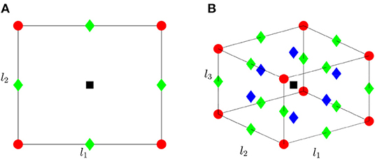
Figure 4. Illustration of (A) two-element and (B) three-element system's stability with element lengths restricted to [l₀, 1]. The global maximum is denoted by a black square, global minima by red circles, and saddle points by diamonds with green indicating an energy of 1 and blue an energy of 2.

3.3. Generalization to Larger Systems

Considering Figure 5, it is clear that the triangular framework can be extended to larger frameworks through addition of pairs of elements to any free edge (Graver, 2001). Provided the lengths of the new elements satisfy the triangle inequality as part of the newly formed triangle, their size can be altered independently. Thus we may describe the energy of such an independent system of N elements through Equation (3). In this case, analogous to the three element system, the energy minima are located precisely at vertices of the hypercube ${\left[l_0,1\right]}^N$. Saddles are located along all 1D edges (these have energy 1) and, more generally, on each face (a hyperplane), with energies determined by the number of unstable elements activated. A single interior maximum is located at the center of the hypercube.

FIGURE 5

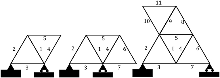
Figure 5. Examples of frameworks with independent elements.

4. Uncoupled Systems. II. Transitions Between Minima

When transitioning between stable states it is often desirable to select the path that minimizes the actuation energy. The barrier to actuation can be considered analogous to the Maxwell energy (see e.g., Hunt et al., 2000b; Wadee and Edmunds, 2005; Champneys et al., 2019). For a system to transition between two minima, it must overcome an energetic barrier, the smallest possible barrier is characterized by one or a series of adjacent saddle points. As individual elements have an activation energy of Π(l_p) = 1, any transition path must encounter an energetic barrier that is at least this magnitude. Thus, for systems of independent elements, the energetically optimal paths between minima are paths traversing the edges of the hypercube ${\left[l_0,1\right]}^N$. Intuitively, such a path makes physical sense, by actuating each element in isolation the individual element's energy barrier is never exceeded.

4.1. Two-Element System

Consider the simple system described in Figure 3A. To ensure the existence of four stable equilibra, we set L_sep = 1. Figure 6A illustrates the energy landscape and shows the expected four stable equilibria and central maximum. The normalized negative gradient, $-\frac{\nabla {\Pi }^N}{\left|\right|\nabla {\Pi }^N\left|\right|}$, in Figure 6B, highlights the stability of the system and matches the expected behavior, Figure 4A.

FIGURE 6

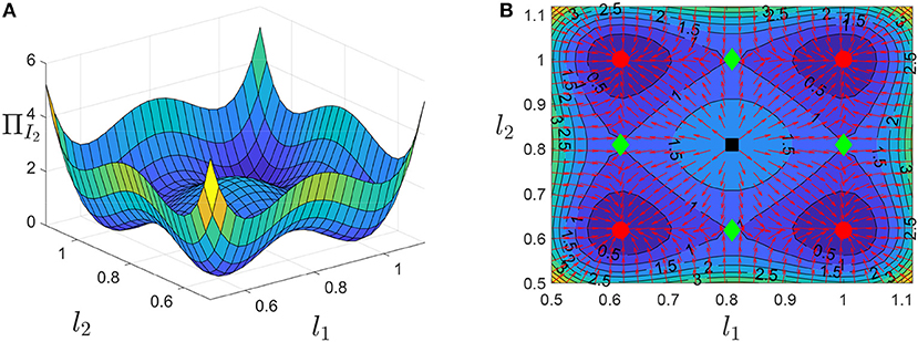
Figure 6. (A) Energy surface for Figure 3A and (B) contour plot with negative normalized gradient. Red circles indicate minima, green diamonds saddle points and the black square a maximum.

A systematic exploration of the domain can be conducted by investigating the transition from a fully contracted to a fully extended configuration, i.e., moving from a configuration where all element lengths are l₀ to one where all lengths are 1. This is always possible for an uncoupled system subject to suitable boundary conditions. This corresponds to two opposite corners of the square domain in Figure 4A. Consider the parametrized path between the two stable configurations given by,

$\begin{array}{ll}\text{l}(t;\alpha )=\left[l_0,l_0,\dots ,l_0\right]+(1-l_0)\left[t^{{\beta }_1},t^{{\beta }_2},\dots ,t^{{\beta }_N}\right]\text{\hspace{1em}with\hspace{1em}}{\beta }_n={\alpha }^{n-1},& (7)\end{array}$

where n ∈ {1, 2, …, N}, α ∈ [1, ∞) and t ∈ [0, 1]. As α → ∞ this curve approaches an edge traversal path. The vertices to be visited along the path can be selected by permuting the order of the powers of t. Owing to the system's symmetry, this is sufficient to explore the entire domain, even though each path sweeps only a portion of the domain. We can define the energy barrier of a path for a given α as,

$\begin{array}{l}{\Pi }_B^N(\alpha )={\displaystyle \underset{t}{max}}{\Pi }^N(\text{l}(t;\alpha )).\end{array}$

However for visualization it is more convenient to use the variable ${\widehat{t}}_K={(1-t)}^{\frac{1}{K}}$, where K ∈ ℕ is a scaling parameter that can be increased as required to account for the number of elements in the system.

Figure 7A illustrates the paths of Equation (7) for a range of α. Figure 7B shows the system's energy during traversal along the path, notably we observe the emergence of two distinct peaks and the reduction in peak magnitude as α increases. Finally, Figure 7C, demonstrates that as the path approaches an edge traversal the energy barrier tends toward 1, i.e., the energetic barrier of actuating a single element.

FIGURE 7

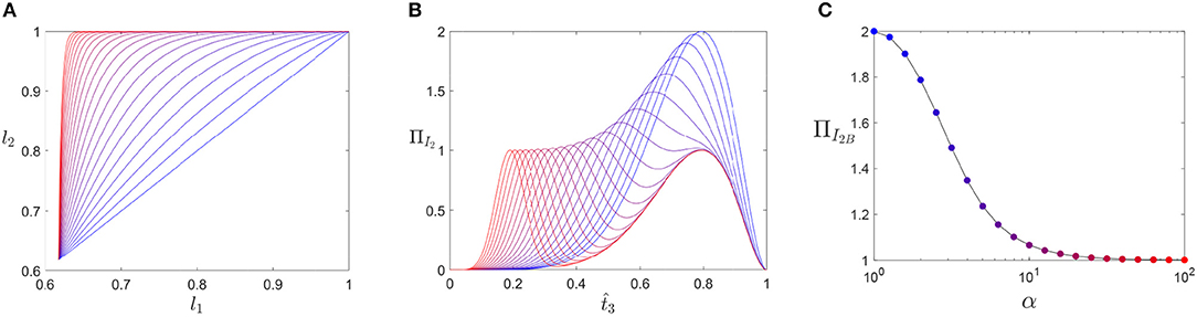
Figure 7. Transition paths for the two-element system in Figure 3A. (A) The path for various α, (B) the energy of system for each path considered, and (C) the maximum energy observed for each path. Line colors in (A,B) transition from blue to red as α increases and correspond to the marker colors in (C).

4.2. Three-Element System

Similarly, for the three-element system in Figure 3A, paths for a range of α are illustrated in Figure 8A. Figure 8B shows the system's energy during the traversal, notably we observe the emergence of three distinct peaks and the reduction in peak magnitude as α is increased. Finally, Figure 8C, demonstrates that as the path approaches an edge traversal the energy barrier tends toward 1.

FIGURE 8

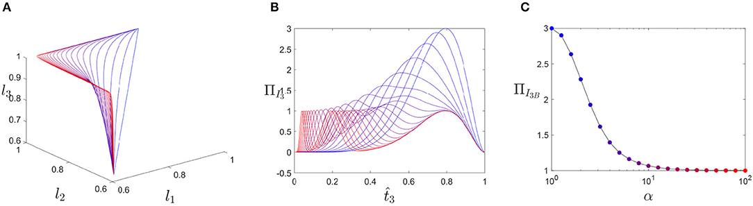
Figure 8. Transition paths for the three-element system in Figure 3B. (A) The path for various α, (B) the energy of system for each path considered, and (C) the maximum energy observed for each path. Line colors in (A,B) transition from blue to red as α increases and correspond to the marker colors in (C).

5. Hexagonal Framework. I. Stable Stress-Free States

We now proceed to analyse a hexagonal framework to illustrate the emergent behavior observed for non-independent systems. Consider six triangles from section 3.1 that form a planar hexagon as illustrated in Figure 9A. In this section we characterize the stable stress-free states of such hexagons.

FIGURE 9

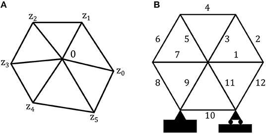
Figure 9. (A) A planar hexagon and (B) a hexagonal system.

We track the positions of the nodes of a hexagon through complex numbers: The central node is at 0 and the other six nodes, numbered anticlockwise, are at z_i ∈ ℂ, i = 0, …, 5, subject to the constraints:

$\begin{array}{ll}\left|z_i\right|\in \left\{l_0,1\right\},& (\mathrm{8a})\end{array}$

$\begin{array}{ll}|z_{i+1}-z_i|\in \left\{l_0,1\right\},& (\mathrm{8b})\end{array}$

where addition of indices is mod 6. Set

$\begin{array}{ll}{w}_i:=\frac{z_{i+1}}{z_i},i=0,\dots ,5,& (9)\end{array}$

so |w_i| is the proportion between the lengths of the adjacent radial edges and argw_i is the interior angle between adjacent radial edges. It follows that a hexagon can be identified with w_i ∈ ℂ, i = 0, …, 5, which satisfy,

$\begin{array}{ll}{\displaystyle \prod _{i=0}^j}{w}_i\in \{l_0,1,\frac{1}{l_0}\},j=1,\dots ,5,& (\mathrm{10a})\end{array}$

$\begin{array}{ll}{\displaystyle \prod _{i=0}^5}{w}_i=1,& (\mathrm{10b})\end{array}$

$\begin{array}{ll}{\displaystyle \sum _{i=0}^5}arg{w}_i=2\pi .& (\mathrm{10c})\end{array}$

With every hexagon we associate a sign diagram, which is a (finite) sequence of signs,

$\begin{array}{ll}{s}_0{s}_1{s}_2{s}_3{s}_4{s}_5,& (\mathrm{11a})\end{array}$

modulo 6-cycle permutations, where

$\begin{array}{ll}{s}_i:=\text{sign}(\left|w_i\right|),& (\mathrm{11b})\end{array}$

as defined in Equation (2).

Now consider the sign diagram Equation (11a), modulo 6-cycle permutations. Note that

1. From Equation (10b), the signs “+” and “−” should occur in equal number.

2. Considered cyclically “+” and “−” should alternate with “0” allowed to intervene, since from Equation (10a) neither two “+”s nor two “−”s can occur sequentially.

From Item 1, there are four classes of sign configurations. These, labeled by the numbers of each sign, are tabulated in Table 1. We now consider each of these configurations.

TABLE 1

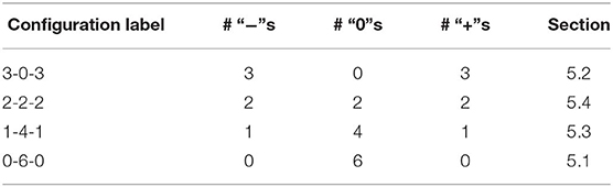
Table 1. The four classes of sign configurations.

5.1. Configuration 0-6-0

The radial edges of the hexagon are of equal length since |w_i| = 1 for i = 0, …, 5.

From section 3.1 and Equation (4) the possible interior angles of the hexagon are ϕ₀₋, $\frac{\pi }{3}$ and ϕ₀₊. Suppose these angles occur with multiplicities q, 6−q−r and r, respectively, for q ∈ {0, …, 6} and r ∈ {0, …, 6 − q}. Then we require

$\begin{array}{ll}q{\varphi }_{0-}+r{\varphi }_{0+}=(q+r)\frac{\pi }{3}\text{\hspace{1em}for }q\in \left\{0,\dots ,6\right\},r\in \left\{0,\dots ,6-q\right\}.& (12)\end{array}$

Since, from Equation (6), ${\varphi }_{0-}<\frac{\pi }{3}<{\varphi }_{0+}$, q = 0 if and only if r = 0. In this case all interior angles are $\frac{\pi }{3}$ and thus the hexagon is regular. On the other hand when q, r ⩾ 1, there is at least one interior angle ϕ₀₋ and at least one interior angle ϕ₀₊. However, this is impossible since ϕ₀₋ cannot occur if all the radial edges are of length l₀ and ϕ₀₊ cannot occur if all the radial edges are of length 1.

Thus, this configuration can be realized only in a regular hexagon. There are two possibilities: Either all edges of the hexagon are of side l₀ or all edges of the hexagon are of side 1.

5.2. Configuration 3-0-3

From Item 2 above, the only possible sequence of signs is

$\begin{array}{l}+-+-+-\end{array}$

considered cyclically. From section 3.1, each interior angle could be either ϕ_±− or ϕ_±+. We can choose p ∈ {0, …, 6} of these to be ϕ_±− provided

$\begin{array}{l}p{\varphi }_{\pm -}+(6-p){\varphi }_{\pm +}=2\pi .\end{array}$

Since, from Equation (6), ${\varphi }_{\pm -}<\frac{\pi }{3}<{\varphi }_{\pm +}$, p ∉ {0, 6}. A numerical investigation shows that the only solution is p = 2 and $l_0=\frac{-1+\sqrt{5}}{2}\approx 0.6180$, which is the inverse golden ratio. A number of hexagons are possible, one of which is illustrated in Figure 10A. However, since we are interested in generic configurations, i.e., those that are feasible for any l₀ ∈ (0.5, 1), henceforth we shall omit details of hexagons that are exist only for some values of l₀.

FIGURE 10

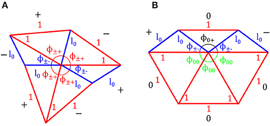
Figure 10. Example hexagon configurations (A) 3-0-3, here l₀ ≈ 0.6180, the inverse golden ratio, so ${\varphi }_{\pm +}=\frac{2\pi }{5}$ and ${\varphi }_{\pm -}=\frac{\pi }{5}$. Note that any three consecutive angles add up to π so geometrically there are three straight lines passing through the central node. (B) 1-4-1 -B^⋆ (see Table 2 for full details).

5.3. Configuration 1-4-1

Modulo multiplication by −1 there are three sub-configurations

$\begin{array}{lllllll}-& +& 0& 0& 0& 0,& (\mathrm{1-4-1\; A})\end{array}$

$\begin{array}{lllllll}-& 0& +& 0& 0& 0,& (\mathrm{1-4-1\; B})\end{array}$

$\begin{array}{lllllll}-& 0& 0& +& 0& 0,& (\mathrm{1-4-1\; C})\end{array}$

considered cyclically. To see this note that we can choose to traverse the circuit such that (i) “−” precedes “+,” and (ii) the number of “0”s between “−” and “+” is no more than the number of “0”s between “+” and “−.” The last sub-configuration is its own negative; the negatives of the first two are

$\begin{array}{lllllll}+& -& 0& 0& 0& 0,& (\mathrm{1-4-1\; -A})\end{array}$

$\begin{array}{lllllll}+& 0& -& 0& 0& 0,& (\mathrm{1-4-1\; -B})\end{array}$

considered cyclically, respectively.

As for interior angles, corresponding to each “−” or “+” we may choose either ϕ_±− or ϕ_±+. Assume, with no loss of generality, that we traverse the interior angles so that the “−” precedes the “+.” Then each “0” between “−” and “+” can be either ϕ₀₀ or ϕ₀₊; and each “0” between “+” and “−” can be either ϕ₀₀ or ϕ₀₋.

We may choose p of ϕ_±−, 2−p of ϕ_±+, q of ϕ₀₋, r of ϕ₀₊ and 4−q−r of $\frac{\pi }{3}$ if

$\begin{array}{lll}p{\varphi }_{\pm -}+(2-p){\varphi }_{\pm +}+q{\varphi }_{0-}=(2+q)\frac{\pi }{3}& \text{for }p=0,1,2,q=0,1,2,3,4;& (\text{for A and -A})\end{array}$

$\begin{array}{lll}p{\varphi }_{\pm -}+(2-p){\varphi }_{\pm +}+q{\varphi }_{0-}+r{\varphi }_{0+}=(2+q+r)\frac{\pi }{3}& \text{for }p=0,1,2,q=0,1,2,3,r=0,1;& (\text{for B and -B})\end{array}$

$\begin{array}{lll}p{\varphi }_{\pm -}+(2-p){\varphi }_{\pm +}+q{\varphi }_{0-}+r{\varphi }_{0+}=(2+q+r)\frac{\pi }{3}& \text{for }p=0,1,2,q=0,1,2,r=0,1,2.& (\text{for C})\end{array}$

Solving the above equations, we deduce that hexagons for Configuration 1-4-1 A are:

1. p = 0, q = 1, r = 0, l₀ ∈ (0.5, 1). There are 4 hexagons for 1-4-1 A and none for 1-4-1 -A.

Hexagons for Configuration 1-4-1 B and 1-4-1 -B are:

1. p = 0, q = 1, r = 0, l₀ ∈ (0.5, 1). There are 3 hexagons for 1-4-1 B and 1 hexagon for 1-4-1 -B.

2. p = 0, q = 3, r = 1, l₀ ≈ 0.6180.

3. p = 1, q = 2, r = 1, $l_0=\sqrt{2-\sqrt{3}}\approx 0.5176$.

4. p = 2, q = 0, r = 1, l₀ ∈ (0.5, 1). There is one hexagon for 1-4-1 B and 3 hexagons for 1-4-1 -B. The first of these, labelled 1-4-1 -B^*, is illustrated in Figure 10B.

Hexagons for Configuration 1-4-1 C are:

1. p = 0, q = 1, r = 0, l₀ ∈ (0.5, 1). There are 2 hexagons.

2. p = 1, q = 2, r = 1, $l_0=\sqrt{2-\sqrt{3}}\approx 0.5176$.

3. p = 2, q = 0, r = 1, l₀ ∈ (0.5, 1). There are 2 hexagons.

4. p = 2, q = 2, r = 2, l₀ ≈ 0.6180.

The generic configurations are listed in Table 2.

TABLE 2

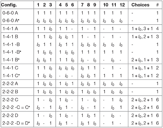
Table 2. The 44 hexagons for generic l₀. Here ^⋆ denotes a hexagon with lengths l₀ and 1 interchanged.

5.4. Configuration 2-2-2

Modulo multiplication by −1 there are four sub-configurations

$\begin{array}{lllllll}-& 0& 0& +& -& +,& (\mathrm{2-2-2\; A})\end{array}$

$\begin{array}{lllllll}-& 0& +& -& 0& +,& (\mathrm{2-2-2\; B})\end{array}$

$\begin{array}{lllllll}-& 0& +& -& +& 0,& (\mathrm{2-2-2\; C})\end{array}$

$\begin{array}{lllllll}-& 0& +& 0& -& +,& (\mathrm{2-2-2\; D})\end{array}$

considered cyclically. To see this note that we can choose to traverse the circuit such that (i) “−” preceeds “+,” and (ii) the first “−” is immediately succeeded by a “0.”

The interior angles are exactly as in Configuration 1-4-1 in section 5.3. Thus, for Sub-Configurations A and B we may choose p of ϕ_±−, 4 − p of ϕ_±+, r of ϕ₀₊ and 2 − r of $\frac{\pi }{3}$ if

$\begin{array}{l}p{\varphi }_{\pm -}+(4-p){\varphi }_{\pm +}+r{\varphi }_{0+}=(4+r)\frac{\pi }{3}\text{\hspace{1em}for }p=0,1,2,3,4,\\ r=0,1,2;\end{array}$

similarly for Sub-Configurations C and D we may choose p of ϕ_±−, 4 − p of ϕ_±+, q of ϕ₀₋, r of ϕ₀₊ and 2 − q − r of $\frac{\pi }{3}$ if

$\begin{array}{l}p{\varphi }_{\pm -}+(4-p){\varphi }_{\pm +}+q{\varphi }_{0-}+r{\varphi }_{0+}=(4+q+r)\frac{\pi }{3}\text{\hspace{1em} for }p=0,1,2,3,4,q=0,1,r=0,1.\end{array}$

Solving the above equations, we deduce that hexagons for Configurations 2-2-2 A and 2-2-2 B are:

1. p = 4, r = 2, l₀ ∈ (0.5, 1). There is one hexagon each for A and B but none for -A and -B.

2. p = 1, r = 0, $l_0=\sqrt{2-\sqrt{3}}\approx 0.5176$.

Hexagons for Configuration 2-2-2 C and 2-2-2 D are:

1. p = 2, q = 1, r = 1, l₀ ∈ (0.5, 1). There are 6 hexagons for each of C, -C, D and -D.

2. p = 1, r = 0, $l_0=\sqrt{2-\sqrt{3}}\approx 0.5176$.

The generic configurations are listed in Table 2.

Having characterized the stable stress-free states of a hexagonal framework we proceed to consider transitions between these states.

6. Hexagonal Framework. II. Energetic Analysis

For a system with independent elements the optimal transition path between minima has an energetic barrier equivalent to actuating each element of the system independently in turn. The design space possess a self-similarity that is retained with increasing numbers of elements. This feature permits physical intuition into the system's behavior. However, systems such as the hexagonal framework, illustrated in Figure 9B, have additional constraints, imposed either by the connectivity of the system or by boundary conditions. We illustrate how the effects of additional constraints can be captured through an additional “geometric” energy.

In a hexagonal framework, we are free to choose the length of 11 of the 12 elements in the system. The 12th element's length then satisfies,

$\begin{array}{ll}{l}_{12}^2=l_1^2+l_{11}^2-2l_1{l}_{11}cos\left({\displaystyle \sum _{j=1}^5}arccos\left(\frac{l_{2j-1}^2+l_{2j+1}^2-l_{2j}^2}{2l_{2j-1}{l}_{2j+1}}\right)\right).& (13)\end{array}$

We proceed therefore to consider the system by way of a perturbation from a 11-element independent system. Using Equation (13) we define a “geometric” energy, ${\Pi }_G:{\left[l_0,1\right]}^{11}\to ℝ$, as the energetic addition owing to the geometric constraints imposed by the system's topology:

$\begin{array}{l}{\Pi }_G(\text{l})=\Pi (l_{12}(\text{l})).\end{array}$

This allows the total energy to be written as

$\begin{array}{l}{\Pi }_C^{11}(l)={\Pi }^{11}(\text{l})+{\Pi }_G(\text{l}).\end{array}$

The analysis in section 5 identified the global minima with zero energy. We note that the system may, in general, possess additional local minima, but these must have an increased energetic state.

Using the approach identified in section 4, a parametric sweep of the 11-dimensional hypercube ${\left[l_0,1\right]}^{11}$ can be conducted. Figure 11 shows the system's energy along the path and the emergence of 11 distinct peaks and convergence of the barrier energy to 1 as the path approaches an edge traversal.

FIGURE 11

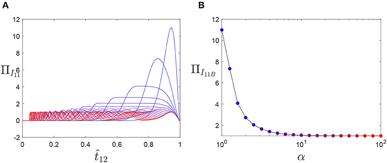
Figure 11. Exploration of transition behavior of the independent 11-element system. (A) describes the energy of system for each path considered as a function of α, and (B) the maximum energy observed for each path. Line colors in (A) transition from blue to red for increasing α and correspond to the marker colors in (B).

We can explore the energy function Π_G in a similar manner, see Figure 12. Unlike the independent case, the system's response is dependent on the relative position of the secondary minimum l₀. There is a significant region of the domain where the energetic barrier does not exceed 1. Geometrically, this indicates that in order for the other independent elements to transition, the dependent length must be extended and contracted in tandem, i.e., there is no path that allows the length of l₁₂ to remain constant. Additionally, this energetic barrier indicates that the actuation path does not require the dependent length l₁₂ to be excessively contracted or extended, but that it may undergo multiple transitions across its own local maximum. Additionally, we observe that as l₀ approaches 0.5 the energy barrier associated with the geometric constraint significantly begins to increase for edge traversal paths. This indicates that in order to accommodate such large geometric reconfiguration the dependent element must be compressed, or extended, significantly. The behavior of the combined system follows from these observations indicating that a path with an energy barrier of 1 cannot be achieved, but that for many geometries an edge traversal remains an effective approach to minimize the energetic cost.

FIGURE 12

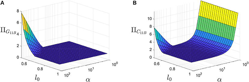
Figure 12. Exploration of transition behavior of the geometric energy of the hexagonal system (A) and total energy (B) as a function of α and l₀.

7. Conclusions

Structural non-linearity offers an expanded design space that can be exploited for the development of adaptive (meta-)materials. The traditional approach to developing transformative (meta-)materials has often relied upon optimization through empirical material science investigations, or the introduction of complex topological structures. Here, instead, we embed non-linearity, in the form of bistability, at the elemental level, recasting the problem as the analysis as simple frameworks of nonlinear springs. In our analysis we investigate the energetic description of these frameworks. In doing so we identify geometric conditions governing the existence of global energetic minima of the system.

Many frameworks can be constructed such that independent variation of the elemental lengths is possible, subject only to satisfaction of the triangle inequality. For these systems, all minima, saddles, and the (unique) maximum, can be obtained directly by considering a hypercube defined by the relative position of the elemental local minima. We use a systematic path search to determine the minimum energetic barrier to transition between self-equilibrated states, analogous to the Maxwell energy. These results support the expected conclusion that actuation of the elements in a sequential manner minimizes the energetic barrier, corresponding to an edge traversal of the hypercube.

For more constrained systems, such as the hexagonal framework we present herein, not all elemental lengths can be selected independently. In these systems, the ratio of the relative positions of elemental local minima determine the geometric feasibility of system-wide global minima. We present the complete set of constraints governing geometric feasibility and identify special elemental ratios that permits adaptive states that are not generically permissible.

In order to explore the transitional behavior of the hexagonal system we consider its energetic description as the combination of independent energy, and an additional “geometric” perturbation. The geometric perturbation arises from the dependency of one elemental length on the remaining 11 elements of the system. Our transitional analysis demonstrates that the dependent element introduces an energetic penalty that cannot be eliminated. That is, we can no longer devise a path that actuates each element in turn. The extent of the energetic penalty is dependent on the elemental ratios, however there are significant regions of the design space that possess nominally identical penalties.

Planar frameworks are of interest even in three-dimensional contexts, e.g., the cross-sectional form of a morphing aerofoil. Moreover, the energetic behavior of uncoupled frameworks is identical in two and three dimensions. For coupled hexagonal systems, as explored in sections 5 and 6, out-of-plane deformations of the nodes may be energetically preferable but, as with the present planar analysis, the system will seek geometrically-preferable configurations that can be identified through global energy minima. The benefits of exploiting non-planar responses of rectangular lattices to develop smart surfaces was explored by Zhang et al. (2017). Three-dimensional frameworks composed of non-linear elements will be considered in future work.

The approach we have presented provides an initial foray into the exploration of the behavior of hierarchical multistable frameworks using a systematic analytical approach. Our approach offers physical intuition into system behavior via two mechanisms. Firstly, the behavior of an independent system can be readily understood owing to its characterization via the hypercube that captures all stable stress-free states. For constrained systems, we can isolate the effects of the constraints, via a perturbation function. By replacing complex topological forms with elements of non-linear stiffness we have provided an alternative approach to tuning global response mechanisms of adaptive (meta-)materials. There is a balance to be struck between elemental non-linearity and topology complexity to yield the most efficient design. This paper begins an exploration of this concept.

Data Availability Statement

The original contributions presented in the study are included in the article, further inquiries can be directed to the corresponding authors.

Author Contributions

MO'D and IC formulated the initial research problem. MO'D, IC, and MT developed the analytical framework. MO'D, IC, and RG conducted the numerical analysis. All authors contributed to the analysis, discussion, and preparation of the manuscript.

Funding

RG was funded by the Royal Academy of Engineering (GB) under the Research Fellowship scheme [Grant No.RF\201718\17178].

Conflict of Interest

The authors declare that the research was conducted in the absence of any commercial or financial relationships that could be construed as a potential conflict of interest.

References

Aza, C., Pirrera, A., and Schenk, M. (2019). Multistable morphing mechanisms of nonlinear springs. J. Mech. Robot. 11:051014. doi: 10.1115/1.4044210

CrossRef Full Text | Google Scholar

Bertoldi, K. (2017). Harnessing instabilities to design tunable architected cellular materials. Annu. Rev. Mater. Res. 47, 51–61. doi: 10.1146/annurev-matsci-070616-123908

CrossRef Full Text | Google Scholar

Bhattacharya, K., and James, R. D. (2005). The material is the machine. Science 307, 53–54. doi: 10.1126/science.1100892

PubMed Abstract | CrossRef Full Text | Google Scholar

Carey, S., Telford, R., Oliveri, V., McHale, C., and Weaver, P. (2019). Bistable composite helices with thermal effects. Proc. R. Soc. A Math. Phys. Eng. Sci. 475:20190295. doi: 10.1098/rspa.2019.0295

PubMed Abstract | CrossRef Full Text | Google Scholar

Champneys, A. R., Dodwell, T. J., Groh, R. M. J., Hunt, G. W., Neville, R. M., Pirrera, A., et al. (2019). Happy catastrophe: recent progress in analysis and exploitation of elastic instability. Front. Appl. Math. Stat. 5:34. doi: 10.3389/fams.2019.00034

CrossRef Full Text | Google Scholar

Che, K., Yuan, C., Wu, J., Qi, H. J., and Meaud, J. (2016). Three-dimensional-printed multistable mechanical metamaterials with a deterministic deformation sequence. J. Appl. Mech. 84:011004. doi: 10.1115/1.4034706

CrossRef Full Text | Google Scholar

Dixon, M., O'Donnell, M., Pirrera, A., and Chenchiah, I. (2019). Bespoke extensional elasticity through helical lattice systems. Proc. R. Soc. A Math. Phys. Eng. Sci 475:20190547. doi: 10.1098/rspa.2019.0547

PubMed Abstract | CrossRef Full Text | Google Scholar

Eßlinger, M. (1970). Hochgeschwindigkeitsaufnahmen vom Beulvorgang dünnwandiger, axialbelasteter Zylinder. Der Stahlbau 39, 73–76.

Google Scholar

Florijn, B., Coulais, C., and van Hecke, M. (2014). Programmable mechanical metamaterials. Phys. Rev. Lett. 113:175503. doi: 10.1103/PhysRevLett.113.175503

PubMed Abstract | CrossRef Full Text | Google Scholar

Graver, J. E. (2001). Counting on Frameworks: Mathematics to Aid the Design of Rigid Structures. Washington, DC: Mathematical Association of America.

Google Scholar

Groh, R. M. J., and Pirrera, A. (2019a). On the role of localisations in buckling of axially compressed cylinders. Proc. R. Soc. A 475:20190006. doi: 10.1098/rspa.2019.0006

PubMed Abstract | CrossRef Full Text | Google Scholar

Groh, R. M. J., and Pirrera, A. (2019b). Spatial chaos as a governing factor for imperfection sensitivity in shell buckling. Phys. Rev. E 100:032205. doi: 10.1103/PhysRevE.100.032205

PubMed Abstract | CrossRef Full Text | Google Scholar

Howell, L. L. (2001). Compliant Mechanisms. New York, NY: John Wiley & Sons.

Google Scholar

Hunt, G., Lord, G., and Champneys, A. (1999). Homoclinic and heteroclinic orbits underlying the post-buckling of axially-compressed cylindrical shells. Comput. Methods Appl. Mech. Eng. 170, 239–251. doi: 10.1016/S0045-7825(98)00197-2

CrossRef Full Text | Google Scholar

Hunt, G., Peletier, M., Champneys, A., Woods, P., Ahmer Wadee, M., Budd, C., et al. (2000a). Cellular buckling in long structures. Nonlin. Dyn. 21, 3–29. doi: 10.1023/A:1008398006403

CrossRef Full Text | Google Scholar

Hunt, G. W., and Dodwell, T. J. (2019). Complexity in phase transforming pin-jointed auxetic lattices. Proc. R. Soc. A Math. Phys. Eng. Sci. 475:20180720. doi: 10.1098/rspa.2018.0720

PubMed Abstract | CrossRef Full Text | Google Scholar

Hunt, G. W., Peletier, M. A., and Wadee, M. A. (2000b). The Maxwell stability criterion in pseudo-energy models of kink banding. J. Struct. Geol. 22, 669–681. doi: 10.1016/S0191-8141(99)00182-0

CrossRef Full Text | Google Scholar

Jutte, C. V., and Kota, S. (2008). Design of nonlinear springs for prescribed load-displacement functions. J. Mech. Design 130:081403. doi: 10.1115/1.2936928

CrossRef Full Text | Google Scholar

Krishnan, G., Kim, C., and Kota, S. (2013). A kinetostatic formulation for load-flow visualization in compliant mechanisms. J. Mech. Robot. 5:021007. doi: 10.1115/1.4023872

CrossRef Full Text | Google Scholar

Lachenal, X., Weaver, P. M., and Daynes, S. (2012). Multi-stable composite twisting structure for morphing applications. Proc. R. Soc. A Math. Phys. Eng. Sci. 468, 1230–1251. doi: 10.1098/rspa.2011.0631

CrossRef Full Text | Google Scholar

Lee, A., López Jiménez, F., Marthelot, J., Hutchinson, J. W., and Reis, P. M. (2016). The geometric role of precisely engineered imperfections on the critical buckling load of spherical elastic shells. J. Appl. Mech. 83:111005. doi: 10.1115/1.4034431

CrossRef Full Text | Google Scholar

Lu, K.-J., and Kota, S. (2003). Design of compliant mechanisms for morphing structural shapes. J. Intell. Mater. Syst. Struct. 14, 379–391. doi: 10.1177/1045389X03035563

CrossRef Full Text | Google Scholar

McHale, C., Carey, S., Hadjiloizi, D., and Weaver, P. M. (2020a). “Morphing composite cylindrical lattices: thermal effects and actuation,” in AIAA Scitech 2020 Forum (Orlando, FL).

Google Scholar

McHale, C., Hadjiloizi, D. A., Telford, R., and Weaver, P. M. (2020b). Morphing composite cylindrical lattices: enhanced modelling and experiments. J. Mech. Phys. Solids 135:103779. doi: 10.1016/j.jmps.2019.103779

CrossRef Full Text | Google Scholar

Mullin, T., Deschanel, S., Bertoldi, K., and Boyce, M. C. (2007). Pattern transformation triggered by deformation. Phys. Rev. Lett. 99:084301. doi: 10.1103/PhysRevLett.99.084301

PubMed Abstract | CrossRef Full Text | Google Scholar

Nadkarni, N., Daraio, C., and Kochmann, D. M. (2014). Dynamics of periodic mechanical structures containing bistable elastic elements: from elastic to solitary wave propagation. Phys. Rev. E 90:023204. doi: 10.1103/PhysRevE.90.023204

PubMed Abstract | CrossRef Full Text | Google Scholar

O'Donnell, M. P., Stacey, J. P., Chenchiah, I. V., and Pirrera, A. (2019). Multiscale tailoring of helical lattice systems for bespoke thermoelasticity. J. Mech. Phys. Solids 133:103704. doi: 10.1016/j.jmps.2019.103704

CrossRef Full Text | Google Scholar

O'Donnell, M. P., Weaver, P. M., and Pirrera, A. (2016). Can tailored non-linearity of hierarchical structures inform future material development? Extreme Mech. Lett. 7, 1–9. doi: 10.1016/j.eml.2016.01.006

CrossRef Full Text | Google Scholar

Pirrera, A., Lachenal, X., Daynes, S., Weaver, P. M., and Chenchiah, I. V. (2013). Multi-stable cylindrical lattices. J. Mech. Phys. Solids 61, 2087–2107. doi: 10.1016/j.jmps.2013.07.008

CrossRef Full Text | Google Scholar

Rafsanjani, A., Akbarzadeh, A., and Pasini, D. (2015). Snapping mechanical metamaterials under tension. Adv. Mater. 27, 5931–5935. doi: 10.1002/adma.201502809

PubMed Abstract | CrossRef Full Text | Google Scholar

Rafsanjani, A., Jin, L., Deng, B., and Bertoldi, K. (2019). Propagation of pop-ups in kirigami shells. Proc. Natl. Acad. Sci. U.S.A. 116, 8200–8205. doi: 10.1073/pnas.1817763116

PubMed Abstract | CrossRef Full Text | Google Scholar

Reis, P. M. (2015). A perspective on the revival of structural (In) stability with novel opportunities for function: from buckliphobia to buckliphilia. J. Appl. Mech. 82:111001. doi: 10.1115/1.4031456

CrossRef Full Text | Google Scholar

Shan, S., Kang, S. H., Raney, J. R., Wang, P., Fang, L., Candido, F., et al. (2015). Multistable architected materials for trapping elastic strain energy. Adv. Mater. 27, 4296–4301. doi: 10.1002/adma.201501708

PubMed Abstract | CrossRef Full Text | Google Scholar

Wadee, M. A., and Edmunds, R. (2005). Kink band propagation in layered structures. J. Mech. Phys. Solids 53, 2017–2035. doi: 10.1016/j.jmps.2005.04.005

CrossRef Full Text | Google Scholar

White, S. C., Weaver, P. M., and Wu, K. C. (2015). Post-buckling analyses of variable-stiffness composite cylinders in axial compression. Compos. Struct. 123, 190–203. doi: 10.1016/j.compstruct.2014.12.013

CrossRef Full Text | Google Scholar

Zhang, J., McInnes, C. R., and Xu, M. (2017). Reconfiguration of a smart surface using heteroclinic connections. Proc. R. Soc. A Math. Phys. Eng. Sci. 473:20160614. doi: 10.1098/rspa.2016.0614

PubMed Abstract | CrossRef Full Text | Google Scholar