A Two-Step Transformation Approach for ESS Model of Viscoelastic Material to Time Domain

ESS (Equivalent Standard solid) model is proofed to be accurate for describing the physical properties of viscoelastic material under different temperatures and excitation frequencies. However, the ESS model faces difficulties for calculating time history responses. Therefore, a two-step transformation approach for ESS model to time domain is proposed, which can obtain precise time history response of structural finite element models of with dampers made of viscoelastic materials. In the first step of the approach, ESS model is extended from frequency domain to complex frequency domain. In the second step, a high-precision numerical inverse Laplace transform method is chosen to transform the model from complex frequency domain to time domain. Experimental and numerical tests are conducted to verify the effectiveness of the two-step transformation approach under simple harmonic external excitation. The comparisons indicate that the approach is accurate under different temperatures and excitation frequencies. Finally, the time domain dynamic responses of the viscoelastic dampers are obtained under earthquake excitations. Comparing to the equivalent linearization method for ESS model, the proposed two-step transformation approach has absolute advantage to obtain accurate results under random excitation, such as earthquake excitations.

Introduction

Viscoelastic material has strong energy dissipation capacity based on massive fillers within high molecular polymers, which exhibits physical properties of both viscous and elastic. When deformations occur under the reciprocating stress, the motion of the matrix molecular chain inside the material will fracture and recombination. In the meantime, mutual friction will occur between the fillers, or between the filler and the matrix. In such physical movement, a part of the energy is stored, and the other part of the energy is converted into thermal energy dissipated to the air (Trindade et al., 2000). The viscoelastic damper is a kind of energy dissipation device used in structural wind-resistant and seismic engineering, which is mainly composed of viscoelastic material and constrained steel plates. The dampers based on viscoelastic material has the characteristics of reliable performance, convenient installation, good damping effect and low cost of produce and maintenance (Park, 2001). However, the physical properties of viscoelastic material are affected significantly greatly by temperature and excitation frequency (Xu et al., 2019). As a result the viscoelastic dampers show strong non-linear characteristics in the working environment. And how to accurately calculate or simulate the mechanical properties of viscoelastic materials is a complex problem (Lewandowski and Chorazyczewski, 2010). A large number of scholars have studied viscoelastic materials and put forward a series of mechanical models, including Maxwell model, Kelvin model, standard solid model (Kim et al., 2003), ESS (equivalent standard solid) model (Xu, 2007; Xu et al., 2011), equivalent stiffness and equivalent damping model (Yoshida et al., 2002), fractional derivative model (Xu et al., 2015), Finite element model, complex stiffness model, Standard rheological model (Mould et al., 2011; Lee and Choi, 2018), fractional index model (Gonzalez et al., 2016; Chen et al., 2018), micro-oscillator model (Mctavish and Hughes, 1993), and so on. The ESS model is a new computational model based on temperature frequency equivalent principle and standard linear solid model, which can correctly describe the variation of viscoelastic damper with the change of temperature and frequency. Besides, the physical concept of the model is clear, and parameters of the ESS model can be quickly obtained through simple harmonic loading tests. As a result, it becomes one of the classical mechanical models of viscoelastic materials in the field of scientific research, and has been widely promoted and applied in engineering (Bhatti, 2013; Xu et al., 2014; Mehrabi et al., 2017; Xu Y. et al., 2017; Xu Z. et al., 2017).

However, the ESS model is the constitutive model based on frequency domain, which needs special mathematical strategy to obtain the time history response under forced vibration or free vibration determined by initial value problem. The most conventional mean current is to use the equivalent linearization method. By the equivalent linearization method, the viscoelastic material is expressed with two constant simplified parameters, i.e., equivalent stiffness and equivalent damping (Park et al., 2007). With the change of dynamic characteristics caused by variation of frequency and temperature, inestimable error will be introduced both in theory or practical application. So the ESS model lose its advantage, which is the high precision for describing the physical property of viscoelastic models. Aiming at the above problems, this paper presents a two-step transformation approach for ESS model of viscoelastic material to time domain, which can accurately obtain the time-domain dynamic response and avoid the establishment of differential equations. The approach directly starts from the frequency domain expressions of the ESS model, and then take two steps to solve the problem. The key innovation of the proposed method is making the ESS model suitable for random excitations. The standard theoretical tools in frequency domain, like the SS model and ESS model, are accurate and simple, but is not applicable in time domain. The standard models in time domain, like fractional derivative model and finite element model, are applicable in time domain, but they are complex in both mathematical formula and experimental tests. The presented model have the advantages in both frequency-domain and time domain, which is the main novel advances of this paper. As a result, the ESS model can be transferred to time domain and produce time history responses of viscoelastic dampers under earthquake excitations or any other stochastic excitations.

Two-Step Transform Approach of ESS Model

The ESS model is suitable in frequency domain, which means it cannot be transformed to time domain directly. In the first step, the ESS model is extended to Laplace domain. In this step the key problem is the imaginary part will cause failure of the second step. As a result the imaginary unit j should be eliminated by certain substitution to prepare for the next step. In the second step, the Laplace expression is transformed to time domain. In this step the key problem is to simplify the formula to reduce the amount of calculation work.

STEP 1

ESS model is a mechanical model describing viscoelastic materials, which can not only describe the influence of performance change with frequency and temperature, but can also describe the relaxation and creep characteristics of viscoelastic dampers. Its expression is known as follows (Xu Y. et al., 2017):

$\begin{array}{l}{G}_1=(q_0+p_1{q}_1{\alpha }_T^c{\omega }^c)\text{/}(1+p_1^2{\alpha }_T^c{\omega }^c)\\ \eta =(q_1-p_1{q}_0){\alpha }_T^d{\omega }^d\text{/}(q_0+p_1{q}_1{\alpha }_T^{2d}{\omega }^{2d})& (1)\end{array}$

In the equation, G₁ represents the energy storage modulus, η is loss factor, ω represents the circular frequency of the excitation load, p₁, q₀, q, c, d, T₀ are the material parameters of the ESS model respectively, which are generally obtained according to the performance test of the representative material. The dissipation modulus G₂ can be obtained from Equation (1):

$\begin{array}{ll}{G}_2=G_{\text{1}}\eta \text{=}\frac{(q_0+p_1{q}_1{\alpha }_T^c{\omega }^c)(q_1-p_1{q}_0){\alpha }_T^d{\omega }^d}{(1+p_1^2{\alpha }_T^c{\omega }^c)(q_0+p_1{q}_1{\alpha }_T^{2d}{\omega }^{2d})}& (2)\end{array}$

The frequency response function H(ω) of the system can be determined by the ESS model, as shown in equation (3):

$\begin{array}{ll}H(\omega )=\frac{\tau (\omega )}{\gamma (\omega )}=G_1(\omega )+\text{j}{G}_2(\omega )& (3)\end{array}$

In the equation, τ is the shear stress of the material, γ is the shear strain of the material, and j indicates the unit imaginary number. Equation (3) belongs to the category of frequency domain, which is a specific form (σ = 0) of Laplace domain (s = σ+jω), so it is necessary to transform the equivalent standard solid model of frequency category to Laplace domain. The frequency response function is transformed into system function H(s), as shown in Equation (4):

$\begin{array}{ll}\begin{array}{c}H(s)=G_1(s)+\text{j}{G}_2(s)\hfill \\ =\frac{(q_0+{\text{j}}^{-c}{p}_1{q}_1{\alpha }_T^c{s}^c)(q_0+{\text{j}}^{-2d}{p}_1{q}_1{\alpha }_T^{2d}{s}^{2d})}{(1+{\text{j}}^{-c}{p}_1^2{\alpha }_T^c{s}^c)(q_0+{\text{j}}^{-2d}{p}_1{q}_1{\alpha }_T^{2d}{s}^{2d})}\\ +\frac{j^{1-d}(q_0+{\text{j}}^{-c}{p}_1{q}_1{\alpha }_T^c{s}^c)(q_1-p_1{q}_{\text{0}}){\alpha }_T^d{s}^d}{(1+{\text{j}}^{-c}{p}_1^2{\alpha }_T^c{s}^c)(q_0+{\text{j}}^{-2d}{p}_1{q}_1{\alpha }_T^{2d}{s}^{2d})}\end{array}& (4)\end{array}$

Both real and imaginary parts exist in the system function as Equation. The transform methods of real part and imaginary part of system function are different, because the imaginary part cannot be transformed to the time domain directly. Some derivation and transformation have to be performed before final transformation. Firstly the real part and imaginary part has to be separated, so the imaginary term j^−−c and j^−2d should be factorized as Equation (5):

$\begin{array}{l}{\text{j}}^{-c}={\left(e^{\text{j}\pi \text{/2}}\right)}^{-c}=e^{\text{j}\pi c\text{/2}}=cos(\pi c\text{/2})-\text{j}sin(\pi c\text{/2})\\ {\text{j}}^{-2d}={\left(e^{\text{j}\pi \text{/2}}\right)}^{-2d}=e^{-\text{j}\pi 2d}=cos(\pi d)-\text{j}sin(\pi d)& (5)\end{array}$

After substituting Equation to Equation, the real and imaginary part of the system function will be separated as Equation (6)

$\begin{array}{ll}H(s)=\text{real}(H(s))+\text{jimag}(H(s))=H_1(s)+\text{j}{H}_2(s)& (6)\end{array}$

where H₁(s) represents the real part, and jH₂(s) represents the imaginary parts of the system function. The physical meaning of Equation (6) is two systems connected in parallel. Because s = σ+jω and σ = 0, so j = s/ω. As a result the imaginary part can be expressed in another form as Equation (7) to transform the imaginary part into time domain.

$\begin{array}{ll}H(s)=H_1(s)+\frac{s}{\omega }{H}_2(s)& (7)\end{array}$

For the real part H₁(s), the system function can be transformed to frequency response function H₁(jω) in frequency domain by letting σ = 0. The frequency response function H₁(jω) can be represented by Equation (8)

$\begin{array}{ll}{H}_1(j\omega )=G_{1\text{\_}1}+j{G}_{1\text{\_}2}& (8)\end{array}$

where G_{1_1} is the storage modulus of the system H₁(s), G_{1_2} is the loss modulus of H₁(s). When sinusoidal excitation u = u₀sin(ωt) applies on the system H₁(s), the output of the system can be expressed as Equation (9)

$\begin{array}{ll}{f}_1(t)=G_{1\text{\_}1}sin(\omega t)+G_{1\text{\_}2}cos(\omega t)& (9)\end{array}$

For the imaginary part jH₂(s), the system function cannot be converted to time domain directly. So at first, we transform H₂(s) in to time domain. The frequency response function H₂(jω) can be represented by Equation (10)

$\begin{array}{ll}{H}_2(j\omega )=G_{2\text{\_}1}+\text{j}{G}_{2\text{\_}2}& (10)\end{array}$

where G_{2_1} is the storage modulus of the system H₂(s), G_{2_2} is the loss modulus of H₂(s). When sinusoidal excitation u = u₀sin(ωt) applies on the system H₂(s), the output of the system g₂(t) can be expressed as Equation (11).

$\begin{array}{ll}g(t)=G_{2\text{\_}1}sin(\omega t)+G_{2\text{\_}2}cos(\omega t)& (11)\end{array}$

As mentioned above, sH₂(s)/ω is chosen to represent jH₂(s).When g(t) is the original function of H₂(s), the inverse Laplace transform of sH₂(s) is f ₂(t) = g′(t), which means the derivative of the original function g(t). So the output of the system can be expressed as Equation (12).

$\begin{array}{ll}{f}_{\text{2}}(t)=\frac{g^{\prime }(t)}{\omega }=-G_{2\text{\_}2}sin(\omega t)+G_{2\text{\_}1}cos(\omega t)& (12)\end{array}$

So the final system output f (t) of the viscoelastic material in time domain can be expressed as Equation (13).

$\begin{array}{l}f(t)=f_1(t)+f_2(t)=(G_{1\text{\_}1}-G_{2\text{\_}2})sin(\omega t)\\ +(G_{1\text{\_}2}+G_{2\text{\_}1})cos(\omega t)& (13)\end{array}$

The above formula (13) shows the expression of the system output of the viscoelastic material under the harmonic excitation. However, the excitation in reality is often a non-harmonic random excitation. The derivation for the time domain response of the viscoelastic material under random displacement excitation is derived in the similar as the system in harmonic excitation. In Laplace domain, the output force of the system can be expressed as Equation (14).

$\begin{array}{ll}\tau (s)=H(s)·\gamma (s)=H_1(s)·\gamma (s)+j{H}_2(s)·\gamma (s)& (14)\end{array}$

where the input displacement γ can be decomposed into a superposition of multiple sinusoidal signals. The decomposition can be realize by Fourier transformation as Equation (15).

$\begin{array}{ll}\gamma (t)={\displaystyle \sum _{n=\text{1}}^{\infty }}{\gamma }_n(n{\omega }_{0}t)=a_0+{\displaystyle \sum _{n=1}^{\infty }}{a}_{n}cosn{\omega }_{0}t+b_{n}sinn{\omega }_{0}t& (15)\end{array}$

where n is the order of Fourier transformation, and ω₀ is the minimum circular frequency of the decomposed signals, and it is correlated with the sampling frequency of the original random signal γ(t). a₀, a_n, b_n are the Fourier coefficients. Then Equation can be modified as Equation (16).

$\begin{array}{ll}\tau (s)=H_1(s)·\gamma (s)+H_2(s)·{\displaystyle \sum _{n=1}^N}\frac{s{\gamma }_n(s)}{{\omega }_n}& (16)\end{array}$

where ω_n = nω₀, which means the circular frequency of the order n of the input signal. Then inverse Laplace transformation is performed on Equation. The following derivation will focus on the invers Laplace transformation of Equation (16).

STEP 2:

After the system function in Laplace domain is obtained, the numerical method of inverse Laplace transformation can be used to obtain the dynamic response in time domain. The direct inversion method is only suitable for simple function which can be decomposed into simple polynomial combination. As for the complexity of the system function of ESS model in Laplace domain, a numerical method is implemented to calculate the inverse transformation (Valsa and Brancik, 1998). The inverse Laplace transform expressions are as follows:

$\begin{array}{ll}f(t)=L^{-1}\left\{F(s)\right\}=\frac{1}{2\pi \text{j}}{\displaystyle {\int }_{\sigma -\text{j}\infty }^{\sigma +\text{j}\infty }}F(s)e^{st}\text{d}s& (17)\end{array}$

Because the upper and lower limits of the integral of Equation (17) contain the positive and negative infinite amount in the imaginary part, it is not possible to integrate Equation (17) directly, so it is necessary to conduct mathematical substitution, if constant a>σt, then |e^−2a+2st| < < 1, so:

$\begin{array}{l}{e}^{st}=\frac{e^{st}}{\text{1}+e^{-\text{2}a+\text{2}st}}=\frac{e^a}{e^{a-st}+e^{-a+st}}\doteq \frac{e^a}{2cosh(a-st)}\\ =\pi e^a{\displaystyle \sum _{n=0}^{\infty }}\frac{{(-1)}^n(n+1/2)}{{(n+1/2)}^2{\pi }^2+{(a-st)}^2}& (18)\end{array}$

The time domain results can be expressed as Equation (19):

$\begin{array}{ll}{f}_c(t,a)=\frac{e^a}{2j}{\displaystyle {\int }_{\sigma -j\infty }^{\sigma +j\infty }}F(s){\displaystyle \sum _{n=0}^{\infty }}\frac{{(-1)}^n(n+1/2)}{{(n+1/2)}^2{\pi }^2+{(a-st)}^2}\text{d}s& (19)\end{array}$

Equation (19) can be simplified to:

$\begin{array}{ll}{f}_c(t,a)=\frac{e^a}{2j}{\displaystyle \sum _{n=0}^{\infty }}{(-1)}^n(n+1/2)I_n& (20)\end{array}$

In which

$\begin{array}{l}{I}_n={\displaystyle {\int }_{\sigma -j\infty }^{\sigma +j\infty }}\frac{F(s)}{{(n+1/2)}^2{\pi }^2+z^2}\text{d}s\\ ={\displaystyle {\int }_{\sigma -j\infty }^{\sigma +j\infty }}\frac{F(s)}{G_n(s)}\text{d}s={\displaystyle {\int }_{\sigma -j\infty }^{\sigma +j\infty }}{K}_n(s)\text{d}s& (21)\end{array}$

In order to solve Equation (21), the original integral path can be regarded as the integral path of the semicircle of the right half plane radius of the coordinate system, so the system singularity points can be obtained as follows:

$\begin{array}{ll}{s}_{1,2}=\frac{a\pm j(n+1/2)\pi }{t}& (22)\end{array}$

The integral along the contour is equal to the sum of the remaining digits of all singularities in the contour, so:

$\begin{array}{l}{I}_n=-2\pi \text{j}\left[\text{re}{\text{s}}_{s=s_1}{K}_n(s)+\text{re}{\text{s}}_{s=s_2}{K}_n(s)\right]\\ =-2\pi \text{j}\left[\frac{F(s_1)}{{G^{\prime }}_n(s_1)}+\frac{F(s_2)}{{G^{\prime }}_n(s_2)}\right]=\frac{F(s_2)-F(s_1)}{t(n+1/2)}\\ =\frac{F\left[a-j(n+1/2)\pi \right]-F\left[a+j(n+1/2)\pi \right]}{t(n+1/2)}& (23)\end{array}$

Finally, the time domain results are obtained:

$\begin{array}{l}{f}_c(t,a)=\frac{e^a}{2j}{\displaystyle \sum _{n=0}^{\infty }}{(-1)}^n(n+1/2)\frac{F(s_2)-F(s_1)}{t(n+1/2)}\\ =\frac{e^a}{2jt}{\displaystyle \sum _{n=0}^{\infty }}{(-1)}^n\left[F(s_2)-F(s_1)\right]& (24)\end{array}$

The system function Equation (16) of the equivalent standard solid model is substituted into the Equation (15) to obtain the final result:

$\begin{array}{ll}{f}_c(t,a)=\frac{e^a}{2jt}{\displaystyle \sum _{n=0}^{\infty }}{(-1)}^n\left[K(s_2)-K(s_1)\right]& (25)\end{array}$

According to Equation (16), the system function H(s) in the complex frequency domain is transformed to the time domain. Under arbitrary input load, the response of the system at any time t can be directly solved by the above functions.

$\begin{array}{ll}{\tau }_c(t,a)=\frac{e^a}{2jt}{\displaystyle \sum _{n=0}^{\infty }}{(-1)}^n\left[\tau (s_2)-\tau (s_1)\right]& (26)\end{array}$

Note that the inverse Laplace transformation on Equation (26) can be simplified. In Equation (16), because γ(t)is the original function of γ(s), so the original function of sγ(s) is γ'(t), which means the derivative of γ(t). As a result, the inverse transform only performed on H₁(s) and H₂(s), the remaining term only need to be derivation and convolution. So the final force output of the viscoelastic material under random displacement excitation can be expressed as Equation (27)

$\begin{array}{ll}\tau (t)=L^{-1}\left[H_1(s)\right]*\gamma (t)+L^{-1}\left[H_2(s)\right]*{\displaystyle \sum _{n=1}^N}\frac{{{\gamma }^{\prime }}_n(t)}{{\omega }_n}& (27)\end{array}$

Where L⁻¹ means the inverse Laplace transform operator, * means the convolution operator.

Validation Under Harmonic Load

In order to verify the correctness of the above method, the preliminary test data of 9050A viscoelastic material in Wuxi Shock absorber Company are analyzed. The 9050A material is composed of high polymer, and is based on Nitrile Butadiene Rubber matrix and vulcanized at high temperature and pressure with variety of additives. The parameters of the material are also listed below. During the experimental test, the temperature is assumed to be uniform in the material, so only the temperature of the surface is measured. According to the test results of the material at different temperature and different frequency, the material parameters are determined by the ESS model, which are, p₁ = 0.0240, q₀ = 2.8440 × 10⁶, q₁ = 5.940 × 10⁵, c = 1.5650, d = 0.7825, T₀ = 45.639^oC. The above parameters will determine the mechanical properties of viscoelastic materials.

The dynamic response of the viscoelastic damper of 9050A viscoelastic material under harmonic displacement excitation is calculated by equivalent linearization method and time domain extension method, respectively. The excitation frequency is 1 Hz, the excitation amplitude is 1 cm, and the force-time curve is shown in Figure 1, the force-displacement curve is shown in Figure 2.

FIGURE 1

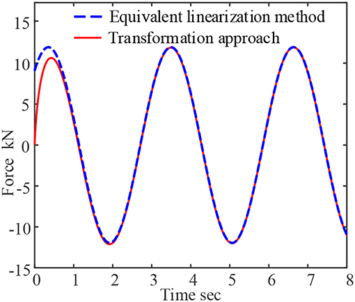
Figure 1. Time history response of viscoelastic damper under harmonic load.

FIGURE 2

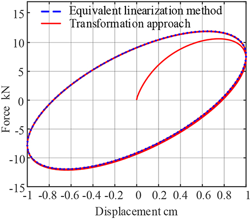
Figure 2. Force-Displacement curve of viscoelastic resistance under harmonic load.

As can be seen from Figures 1, 2, the results are different at the initial moment between the proposed approach and equivalent linearization method. The force response obtained by the proposed approach starts from the origin point, which reflects the relaxation characteristics of viscoelastic materials. The stress relaxation phenomenon is important in viscoelastic materials. When displacement is applied on a system with stress relaxation behavior, the output force of should start from 0, which is proved by Maxwell model. The Maxwell model is good at predicting the stress relaxation phenomenon by akin to a spring being in series with a dashpot. In contrast, the equivalent linearization model cannot reflect the relaxation response of viscoelastic materials. In addition, the results of the two methods tend to be equal after about 1 s, which indicates that the steady-state solution of the two-step transformation approach is correct.

The calculation formula of the storage modulus G₁ and the loss factor η from the force-displacement hysteresis curve is as follows:

$\begin{array}{l}{G}_1=\frac{2E}{{\gamma }_0^2}\\ \eta =\frac{E_d{\gamma }_0^4}{2\pi E}& (28)\end{array}$

Where E_d represents the area surrounded by the force-displacement hysteresis curve, E represents the strain energy stored when the material produces the maximum strain γ₀, and γ₀ represents the maximum strain of the material. According to formula (17), in the case of the viscoelastic dampers at a temperature of −10^oC, 0^oC, 10^oC, 20^oC, under the input frequency for 0.1, 0.5, 1, 2 rad, the storage modulus and loss factor test and theoretical analysis of the results of the comparison can be calculated and as shown in Table 1. From the table, the comparison of the calculation results between the proposed approach and the equivalent linearization method, the maximum error of the energy storage modulus G₁ is 0.0054%, the maximum error of the loss Factor η is 0.2797%, and the error analysis indicates that the time domain extension method has sufficient precision for solving the solution. Note that the comparison is between the ESS model and the proposed two-step transformation approach. There are limitations of the ESS model that it cannot be used under earthquake excitations. So the two-step transformation approach is proposed to conquer this shortage. The comparison between ESS model and the proposed method indicates that the proposed method is indeed transferring the ESS model to time domain without bring much errors.

TABLE 1

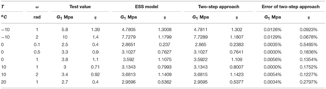
Table 1. Calculation results of 9050A models of viscoelastic materials.

Validation Under Random Excitation

The two-step transformation approach adopts exactly the same mathematical strategy to process both harmonic and earthquake excitations. The comparisons under harmonic excitation indicate that not only the results under harmonic excitation is correct, but also the total mathematical strategy is accurate. So the results under earthquake excitation is also accurate, because it adopts the same accurate mathematical strategy. In other words, the mathematical formulas of the two-step transformation approach cannot tell the difference between harmonic signals and earthquake signals, which are both a series of different numbers. As a result, if the approach dealt with harmonic number correctly, they must dealt with earthquake signals correctly. Both El Centro and Taft earthquake waves are chosen as excitations to verify the applicability of the proposed method.

The equivalent linearization method is also adopted in the following comparisons because it is based on ESS model and is usually adopted to calculate the response of viscoelastic material. Although the equivalent linearization method will bring errors to the system, it is simple and practical. The comparisons can quantify the exact error that the equivalent linearization method brings to the system.

Validation Under El Centro Earthquake Wave

The two-step transformation approach is used to calculate the response of the Viscoelastic damper under the El-Centro earthquake excitation with 400 gal amplitude. The time history curve of force is shown in the red solid line in Figure 3. The force-displacement cure is shown in the red solid line in Figure 4. At the same time, equivalent linearization method is used to make approximate calculation on the viscoelastic system. The equivalent linearization method assumes that the system works under simple harmonic loads of fixed frequency, and the excitation frequency usually equals to the nature frequency of the system. In this working condition, the frequency of the equivalent linearization method assumes to be 0.2 and 5 Hz, respectively.

FIGURE 3

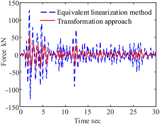
Figure 3. Force-time curve of viscoelastic damper under seismic load (assuming working frequency is 0.2 Hz).

FIGURE 4

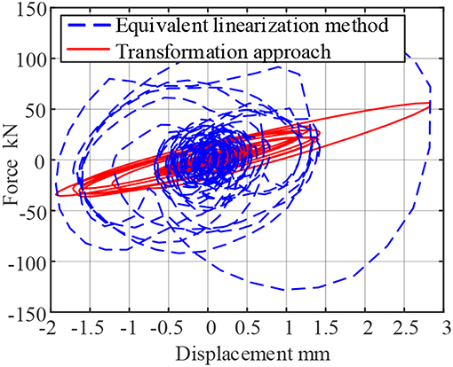
Figure 4. Force-Displacement curve of viscoelastic resistance under seismic load (assuming working frequency is 0.2 Hz).

For example, when the assuming frequency is 0.2 Hz, the equivalent linearization method considers that the damper's operating frequency is ω = 2πf = 1.2566 rad. So based on the assumptions, the storage modulus G₁ = 5.5113 × 10⁶ Pa, Loss factor η = 1.2998, and the time history curve of force and force-displacement curves of the damper are plotted as shown in the blue dashed lines of Figures 3, 4.

Through comparisons, the maximum output of the system calculated by the two-step transformation approach is 56.2315 kN, and the maximum output of the damper calculated by the equivalent linearization method is 124.6607 kN, and the proposed method improve the system accuracy by 121.69%. The force-displacement curve can also be found that the hysteresis loop calculated by the equivalence method is extremely full, so the energy dissipation effect of the damper is overestimated, which is an unsafe behavior in engineering design.

When the working frequency of the viscoelastic system is assumed to be 5 Hz, the equivalent linearization method considers that the working frequency of the system is ω = 2πf = 31.4159 rad, so it can be calculated based on the assumption that the storage modulus G₁ = 23.7705 × 10⁶ Pa, loss factor η = 0.1905, The force-time curve and force-displacement curve of the viscoelastic system are shown in the blue dashed lines of Figures 5, 6.

FIGURE 5

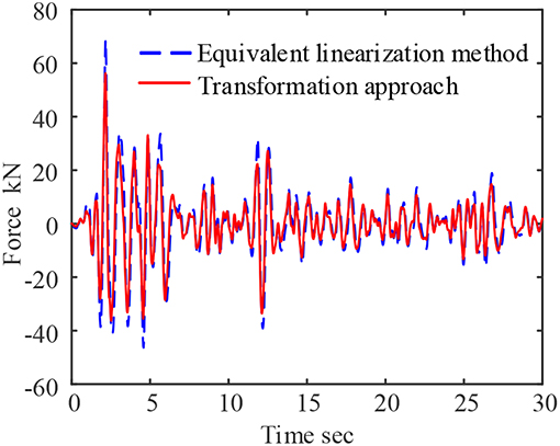
Figure 5. Force time curve of viscoelastic damper under seismic load (assuming working frequency 5 Hz).

FIGURE 6

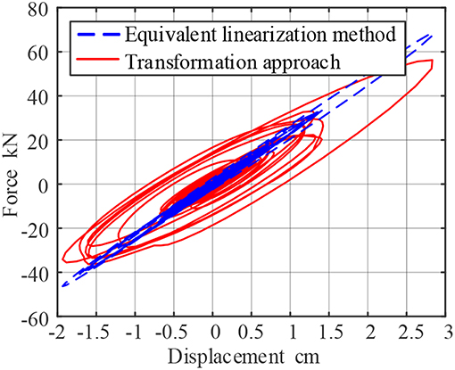
Figure 6. Force-Displacement curve of viscoelastic resistance under seismic load (assuming working frequency 5 Hz).

Through comparisons, it is concluded that the maximum output force of the damper calculated by the proposed approach is 56.2315 kN, and the maximum output force of the damper calculated by the equivalent linearization method is 68.7177 kN. The proposed method improve the system accuracy reaches 22.2%. The force-displacement curve can also concludes that the hysteresis loop of the equivalent linearization method is not full and the slope increases. It is shown that the equilibration method underestimates the energy consumption effect of the damper, and overestimates the stiffness of the damper, which is quite different from the real result.

In addition, when the frequency is 0.2 Hz, it means the first frequency of the system is assumed to be 0.2 Hz for equivalent linearization method. This condition is usually suitable for the high rise building which is soft. On the other hand, 5 Hz means the period of the structure is 0.2 s which means the structure is low and stiff. For viscoelastic material, the loss factor decreases with increasing frequency, so the curve in high frequency is not as full as in low frequency.

Validation Under Taft Earthquake Wave

In order to verify the universality of the proposed two-step transformation approach. Taft earthquake excitation with 400 gal amplitude is chosen as the input excitation on the viscoelastic system. The force time history curve of the damping system is shown in the red solid line in Figure 7. The force-displacement cure is shown in the red solid line in Figure 8. At the same time, equivalent linearization method is used to make estimation of the response of the viscoelastic system. The working frequency of the approximate method is also assumed to be 0.2 and 5 Hz, respectively.

FIGURE 7

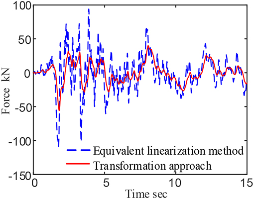
Figure 7. Force-time curve of viscoelastic damper under seismic load (assuming working frequency is 0.2 Hz).

FIGURE 8

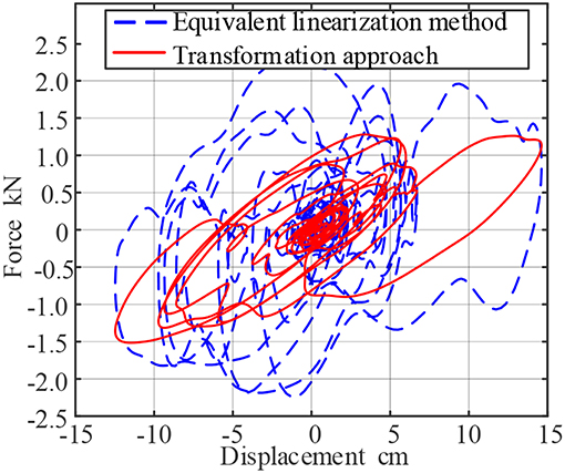
Figure 8. Force-Displacement curve of viscoelastic resistance under seismic load (assuming working frequency is 0.2 Hz).

As mentioned before, when the assuming working frequency is 0.2 Hz, the equivalent linearization method considers that the damper's working frequency is ω = 2πf = 1.2566 rad, and the calculated energy storage modulus G₁ = 5.5113 × 10⁶ Pa, Loss factor η = 1.2998, the time history curve of force and force-displacement curves of the damper are calculated as shown in the blue dotted lines of Figures 7, 8.

Through comparison, the maximum output of the viscoelastic system calculated by the two-step transformation approach is 55.7772 kN, and the maximum output of the damper calculated by the equivalent linearization method is 108.7909 kN, and the proposed method improve the system accuracy reaches 95.05%. The same as El Centro earthquake, the force-displacement curve of Taft earthquake wave can also be found that the hysteresis loop calculated by the equivalence method is extremely full, and the energy dissipation effect of the damper is overestimated, which is an unsafe behavior in engineering design.

When the operating frequency of the damper is assumed to be 5 Hz, the equivalent linearization method considers that the operating frequency of the damper is ω = 2πf = 31.4159 rad, and the calculated storage modulusG₁ = 23.7705 × 10⁶ Pa, loss factor η = 0.1905, The force-time curve and force-displacement curve for calculating the damper are shown in the blue dashed lines of Figures 9, 10.

FIGURE 9

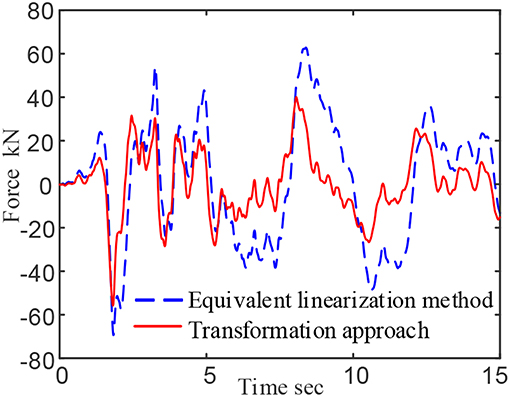
Figure 9. Force time curve of viscoelastic damper under seismic load (assuming working frequency 5 Hz).

FIGURE 10

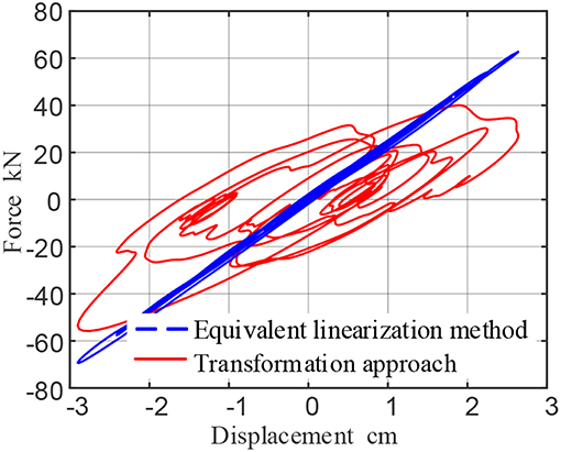
Figure 10. Force-Displacement curve of viscoelastic resistance under seismic load (assuming working frequency 5 Hz).

Through comparison, it is concluded that the maximum output force of the damper calculated by the proposed approach is 55.7772 kN, and the maximum output force of the damper calculated by the equivalent linearization method is 69.3388 kN. The proposed method improve the system accuracy reaches 24.31%.

Same as El Centro earthquake, the force-displacement curve under Taft earthquake can also be found that the hysteresis loop of the equivalent linearization method is not full, and the slope increases. It is also shown that the equilibration method underestimates the energy consumption effect of the damper, and overestimates the stiffness of the damper, which is quite different from the real result.

In addition, because the ESS model is only suitable for harmonic signal, so an equivalent linearization method is usually adopted to extend the ESS model to time domain. However, the equivalent linearization method is approximate, and the two-step transformation approach is more accurate. As a result, the difference is large when using earthquake excitation. The equivalent linear model can only deal with signals with one frequency, while the earthquake contain plenty of frequencies. So only one representative frequency of earthquake waves is choose to perform the calculation. That's the reason why the equivalent linearization method is approximate and inaccurate, and why the two-step transformation approach is proposed.

Conclusion and Prospect

In this paper, a two-step transformation approach is used to calculate the response of the viscoelastic damper under the El-Centro earthquake excitation. The proposed approach avoids the establishment of complex time-domain differential equations, which can start directly from the frequency domain expression of the ESS model of viscoelastic materials, and calculate the time domain response of viscoelastic materials under harmonic excitation and seismic excitation.

The following conclusions are drawn by experimental tests and numerical solutions:

(1) The proposed method can accurately calculate the ESS model in the time domain range. The comparison calculation results show that the error is small, the maximum error of the energy storage modulus G₁ 0.0054%, and the maximum error of the loss Factor η 0.2797%.

(2) The traditional solution method with equivalent stiffness and equivalent damping will bring large errors, when it is assumed that ω is large, the hysteresis loop is very full calculated by the equivalence method, the energy dissipation effect of the damper is overestimated, and when the ω is assumed to be small, the energy dissipation effect of the damper is estimated low. On the other hand, the stiffness of the damper is over estimated. The engineers is encouraged to use the two-step transformation approach to evaluate and predict the mechanical properties of viscoelastic materials.

(3) In the current stage, the two-step transformation approach under random earthquakes is mainly verified by numerical results. The future research will focus on the experimental verification under random excitations. Also the accuracy of the models should be improved and the computation cost should be reduced in the following research.

Data Availability

The raw data supporting the conclusions of this manuscript will be made available by the authors, without undue reservation, to any qualified researcher.

Author Contributions

All authors listed have made a substantial, direct and intellectual contribution to the work, and approved it for publication.

Conflict of Interest Statement

The authors declare that the research was conducted in the absence of any commercial or financial relationships that could be construed as a potential conflict of interest.

Acknowledgments

Financial supports for this research are provided by National Natural Science Foundation of China (56237845), Natural Science Foundation of Jiangsu Province (BK20170684), National Key R&D Program Key Special Project (2016YFE0200500), National Key R&D Program Project Funding (2016YFE0119700), and Fundamental Research Funds for the Central Universities (2242017K40215). These supports are gratefully acknowledged.

References

Bhatti, A. Q. (2013). Performance of viscoelastic dampers (VED) under various temperatures and application of magnetorheological dampers (MRD) for seismic control of structures. Mech. Time-Depend. Mat. 17, 275–284. doi: 10.1007/s11043-012-9180-2

CrossRef Full Text | Google Scholar

Chen, S., Liu, F., Turner, I., and Hu, X. (2018). Numerical inversion of the fractional derivative index and surface thermal flux for an anomalous heat conduction model in a multi-layer medium. Appl. Math. Model. 59, 514–526. doi: 10.1016/j.apm.2018.01.045

CrossRef Full Text | Google Scholar

Gonzalez, E. A., Castro, M. J. B., Presto, R. S., Radi, M., and Petras, I. (2016). “Fractional-order models in motor polarization index measurements,” in 17th International Carpathian Control Conference (ICCC). (Tatranská Lomnica), 214–217. doi: 10.1109/CarpathianCC.2016.7501096

CrossRef Full Text | Google Scholar

Kim, J., Choi, H., and Min, K. W. (2003). Performance-based design of added viscous dampers using capacity spectrum method. J. Earthq. Eng. 7, 1–24. doi: 10.1080/13632460309350439

CrossRef Full Text | Google Scholar

Lee, D. K., and Choi, M. S. (2018). Standard reference materials for cement paste, part I: suggestion of constituent materials based on rheological analysis. Materials 11:1040624. doi: 10.3390/ma11040624

PubMed Abstract | CrossRef Full Text | Google Scholar

Lewandowski, R., and Chorazyczewski, B. (2010). Identification of the parameters of the Kelvin-Voigt and the Maxwell fractional models, used to modeling of viscoelastic dampers. Comput. Struct. 88, 1–17. doi: 10.1016/j.compstruc.2009.09.001

CrossRef Full Text | Google Scholar

Mctavish, D. J., and Hughes, P. C. (1993). Modeling of linear viscoelastic space structures. J. Vib. Acoust. 115, 103–110. doi: 10.1115/1.2930302

CrossRef Full Text | Google Scholar

Mehrabi, M. H., Suhatril, M., Ibrahim, Z., Ghodsi, S. S., and Khatibi, H. (2017). Modeling of a viscoelastic damper and its application in structural control. PLoS ONE 12:e0176480. doi: 10.1371/journal.pone.0176480

PubMed Abstract | CrossRef Full Text | Google Scholar

Mould, S, Barbas, J, Machado, A. V, Nóbrega, J. M, and Covas, J.A. (2011). Measuring the rheological properties of polymer melts with on-line rotational rheometry. Polym. Test. 30, 602–610. doi: 10.1016/j.polymertesting.2011.05.002

CrossRef Full Text | Google Scholar

Park, J., Min, K., Chung, L., Lee, S., Kim, H., and Moon, B. (2007). Equivalent linearization of a friction damper-brace system based on the probability distribution of the extremal displacement. Eng. Struct. 29, 1226–1237. doi: 10.1016/j.engstruct.2006.07.025

CrossRef Full Text | Google Scholar

Park, S. W. (2001). Analytical modeling of viscoelastic dampers for structural and vibration control. Int. J. Solids Struct. 38, 8065–8092. doi: 10.1016/S0020-7683(01)00026-9

CrossRef Full Text | Google Scholar

Trindade, M. A., Benjeddou, A., and Ohayon, R. (2000). Modeling of frequeney-dependent viscoelastic materials for active-passive vibration damping. J. Vib. Acoust. 122, 169–174. doi: 10.1115/1.568429

CrossRef Full Text | Google Scholar

Valsa, J., and Brancik, L. (1998). Approximate formulae for numerical inversion of Laplace transforms. Int. J. Numer. Model. El. 11, 153–166. doi: 10.1002/(SICI)1099-1204(199805/06)11:3<153::AID-JNM299>3.0.CO;2-C

CrossRef Full Text | Google Scholar

Xu, Y., Xu, Z., Ge, T., and Xu, C. (2017). Equivalent fractional order micro-structure standard linear solid model for viscoelastic materials. Chin. J. Theor. Appl. Mech. 49, 1059–1069. doi: 10.6052/0459-1879-17-134

CrossRef Full Text

Xu, Z. (2007). Earthquake mitigation study on viscoelastic dampers for reinforced concrete structures. J. Vib. Control 13, 29–43. doi: 10.1177/1077546306068058

CrossRef Full Text | Google Scholar

Xu, Z., Gai, P., Zhao, H., Huang, X., and Lu, L. (2017). Experimental and theoretical study on a building structure controlled by multi-dimensional earthquake isolation and mitigation devices. Nonlinear Dyn. 89, 723–740. doi: 10.1007/s11071-017-3482-5

CrossRef Full Text | Google Scholar

Xu, Z., Huang, X. H., Xu, F. H., and Yuan, J. (2019). Parameters optimization of vibration isolation and mitigation system for precision platforms using non-dominated sorting genetic algorithm, Mech. Syst. Signal Process. 128, 191–201. doi: 10.1016/j.ymssp.2019.03.031

CrossRef Full Text | Google Scholar

Xu, Z., Wang, D., and Shi, C. (2011). Model, tests and application design for viscoelastic dampers. J. Vib. Control 17, 1359–1370. doi: 10.1177/1077546310373617

CrossRef Full Text | Google Scholar

Xu, Z., Wang, S., and Xu, C. (2014). Experimental and numerical study on long-span reticulate structure with multidimensional high-damping earthquake isolation devices. J. Sound Vib. 333, 3044–3057. doi: 10.1016/j.jsv.2014.02.013

CrossRef Full Text | Google Scholar

Xu, Z., Xu, C., and Hu, J. (2015). Equivalent fractional Kelvin model and experimental study on viscoelastic damper. J. Vib. Control 21, 2536–2552. doi: 10.1177/1077546313513604

CrossRef Full Text | Google Scholar

Yoshida, N., Kobayashi, S., Suetomi, I., and Miura, K. (2002). Equivalent linear method considering frequency dependent characteristics of stiffness and damping. Soil Dyn. Earthq. Eng. 22, 205–222. doi: 10.1016/S0267-7261(02)00011-8

CrossRef Full Text | Google Scholar