Seasonal spatial distribution patterns of AmphiOctopus ovulum in the East China Sea: current status future projections under various climate change scenarios

Currently, there is also little up to date information on the the current population status and life history traits of AmphiOctopus ovulum, a very often seen cephalopod species in the East China Sea. It is therefore important to figure out the seasonal spatial distribution of this species, both in terms of number and biomass, and the environmental variables which determine them. Additionally, climate change plays an important role in determining the characteristics of individual species and thus on the ecosystems they inhabit. We set out to understand the responses of A. ovulum to habitat variables and to make projections based on the climate change scenarios described in the IPCC’s SSP1-2.6 and SSP5-8.5 criteria. We carried out seasonal bottom trawling surveys in the East China Sea region during 2018 and 2019 to fill this knowledge gap. Our results showed that the average individual size values ranged from 17.80−43.00 g·ind^-1 in spring and 23.49−33.00 g·ind^-1 in summer; the measured sea bottom temperature, sea bottom salinity, and depth value ranges were 10.81−27.06°C, 31.73–35.25‰, and 91–103 m independently in spring to winter. Our study showed that A. ovulum was distributed in the area between 27°–29°N, 122.5°–125°E during spring to autumn, and expanded into the area between 26.5°–32.5°N, 121°–124.5°E in winter. The core habitat of A. ovulum was centered on the area between 27.5°–28°N, 122.5°–123.5°E, and can be expected to expand to the northeast and southwest independently under the most likely global warming scenarios. Our results will benefit the development of suitable conservation measures for cephalopod habitats, and incorporate the impacts of climate change into fisheries management programs.

1 Introduction

Cephalopods form a vital part of marine ecosystems and have become commercially fished species in recent years. The FAO (2024) has reported that cephalopod catches reached a record of 3.90 million tonnes; in 2022, global cephalopod exports, including the taxa of octopus, squid, and cuttlefish, reached USD 14.30 billion, constituting 7.00% of the world’s total exports of aquatic animal products. A limited supply of octopus resulted in price increases after the COVID-19 pandemic (FAO, 2024). In contrast, populations of traditionally targeted, higher trophic level, economic fish species have been in continuous decline due to overfishing during recent decades, to the benefit of cephalopod populations (Rosa et al., 2019).

In China, the catches of Sepiella japonica have historically exceeded over 70,000 t annually in the East China Sea region (Qin et al., 2011). Prior to the 1970s the larger cephalopod species such as Sepiella maindroni, Sepia esculenta, Sepia latimanus, and Sepia pharaonis were the most caught species (Li et al., 2006). After the 1990s, the dominant species caught were Todarodes pacificus and Uroteuthis edulis, replacing S. maindroni, and after 2006 Octopus spp. became the focus of the fishing industry, especially in the coastal areas of the East China Sea (Zhu et al., 2014). (Liang et al. (2025) suggested that A. fangsiao was one of dominant species in Zhejiang coastal areas (Liang et al., 2025).

The benthic temperate species AmphiOctopus ovulum, is found in warm water areas, mainly in the Northwest Pacific including China and Japan. It inhabits the sea bottom in shallow areas, and releases eggs that attach to the stipes of macroalgae. Male and female adult individuals usually die shortly after spawning and brooding; embryos hatch into a planktonic stage and live for some time before they grow larger, and adopting a benthic lifestyle. No significant differences in genetic characteristics or life history traits have been found between populations inhabiting different geographical areas (Dou, 2017). Pang et al. (2020) suggested that AmphiOctopus fangsiao may migrate short distances along with seasonal changes and coastal currents (Pang et al., 2020).

In general, little is known about the species’ ecology and biology, especially regarding its seasonal spatial distribution patterns and characteristics. Furthermore, local fishermen are generally not able to distinguish the various Octopus spp. and combine them all together in their catch data reports to the government. For this reason, independent scientific survey data is important to understand the habitat distribution of A. ovulum.

In addition, climate change has increased since the 1850s (Checkley et al., 2017). In aquatic ecosystems, rising atmospheric CO2 levels are driving rapid climate changes (Le Quere, 2010). Atmospheric pCO2 increased from a preindustrial concentration of 280 ppm to more than 400 ppm (Keeling, 2016), whereas the seawater pH decreased by 0.11 units (IPCC (Intergov. Panel Clim. Change), 2013). Atmospheric CO2 concentrations are expected to reach 1000 ppm by the end of the current century (IPCC (Intergov. Panel Clim. Change), 2013). Demersal aquatic animals such as A. ovulum are often more vulnerable to climate change than pelagic aquatic animal communities (Zhu et al., 2022). Climate change can affect individuals and schools of aquatic animals, and consequently influence fisheries (Zhu et al., 2022). Yang et al. (2025) suggested that the annual mean habitat area of A. fangsiao will decrease under SSP1-2.6 by 2050, and increase under SSP1-2.6 by 2100 (Yang et al., 2025).

This study set out to assess the seasonal spatial distribution patterns of A. ovulum and correlate them with environmental variables, to understand how their habitats and distribution patterns may change under different climate scenarios. Our results should improve the conservation management efforts for this species. A better understanding of its distribution patterns is essential to understand the influences of environmental variables on this species, and to aid in improving ecosystem-based fisheries management strategies.

2 Method

2.1 Study areas and procedures

Independent scientific bottom trawling surveys were conducted in the southern Yellow and East China Seas during 2018 and 2019. The surveys used a trawl net with a cod end mesh size of 20.00 mm, towed by fisheries research vessels (the Zhongkeyu 211 and 212) in autumn (2–11 November 2018: 854.40 g·h−1 of total CPUEw and 38.50 ind·h−1 of total CPUEn), winter (4–27 January 2019: 883.96 g·h−1 of total CPUEw and 23.04 ind·h−1 of total CPUEn), spring (22 April–10 May 2019: 226.40 g·h−1 of total CPUEw and 6.00 ind·h−1 of total CPUEn), and summer (13 August–27 September 2019: 560.15 g·h−1 of total CPUEw and 19.54 ind·h−1 of total CPUEn). The study area covered 26.50°–35.00°N, 120.00°–127.00°E, and survey stations were determined using a sampling grid with dimensions of 30 min of latitude and 30 min of longitude (30’×30’) (Figure 1). The average trawl speed was three knots and all tows were conducted for 1 h duration at each station. The catches were analyzed in the laboratory to identify the species caught and assess their occurrence at each station. Each species was counted and weighed to the nearest 0.10 g of wet weight, and their catch density was calculated as biomass density per unit of sampling time (units: g·h−1) and density per unit of sampling time (units: ind·h−1). We identified the species of A. ovulum according to morphological characteristics including a near-oval brown-black patch with a purple circle inside it, located below the eyes, between the second and third wrist pair. Environmental variables, including water depth, water temperature, and salinity were collected at each station using a conductivity-temperature-depth profiler (SBE-19; SeaBird-Scientific, Bellevue, WA, USA) (Xu et al., 2023). The sea surface temperature (SST) and salinity (SSS) were measured at 3 m below the surface, and the sea bottom temperature (SBT) and sea bottom salinity (SBS) were measured 2.00 m above the sea bottom (at sea depths< 50.00 m) and 2.00–4.00 m above the bottom (at sea depths > 50 m). Ottersen et al. (2010) suggested that the oceanographic parameters of the sea surface are very important for ocean circulation patterns, vertical mixing, availability of nutrients, and subsequent marine ecosystem primary production, which appear to be the leading indicators and important drivers of marine fishery resource fluctuations (Ottersen et al., 2010). The average individual weight (AIW) was defined as the CPUE by weight (CPUEw) divided by the CPUE by number (CPUEn), at each station.

Figure 1

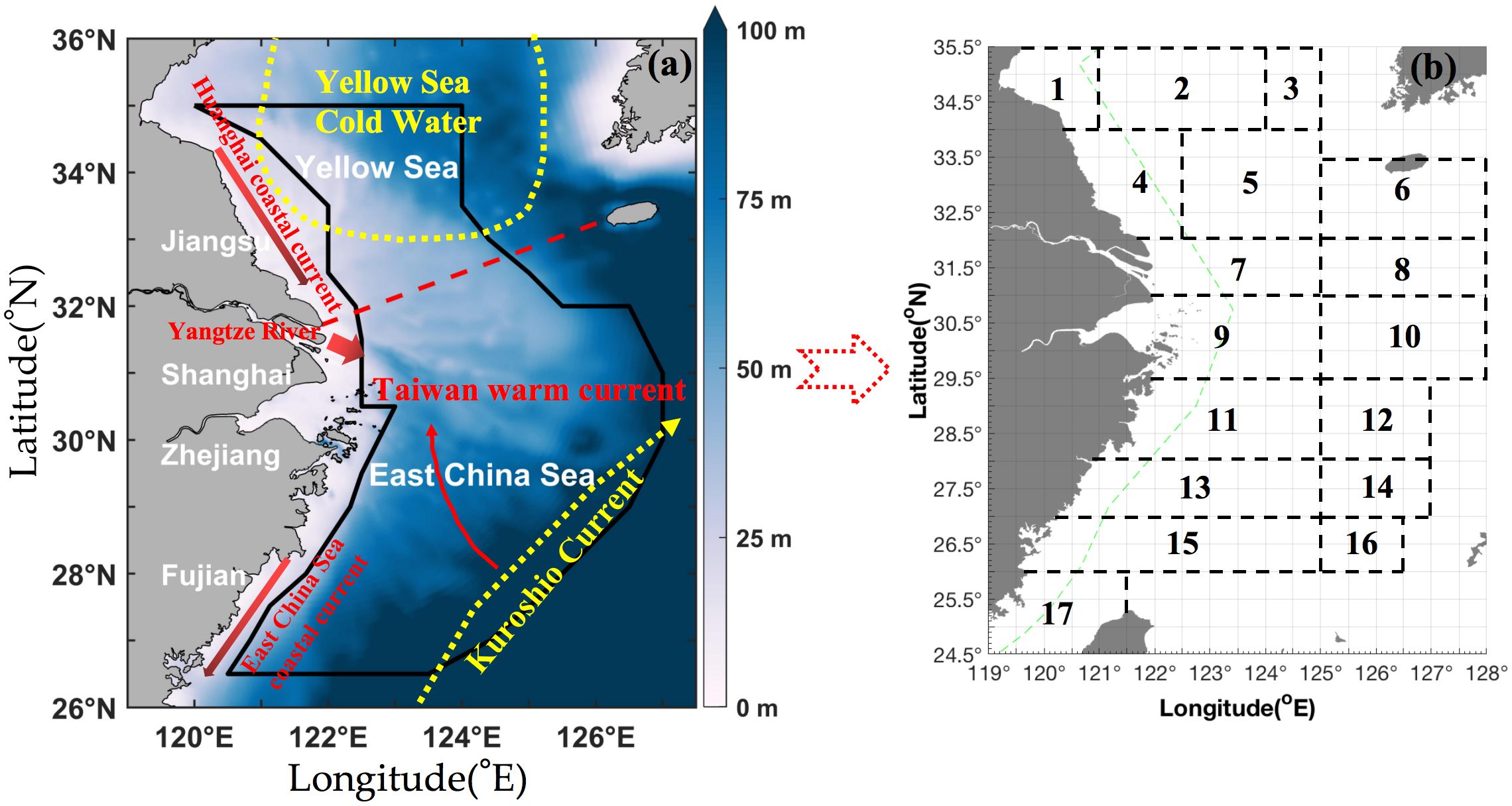
Figure 1. Survey map information. (a) Map of the survey area (26.50° N–35.00° N 120.00° E–127.00° E), which is denoted by a dark blue solid line in the East China Sea region, including the Southern Yellow and East China Seas adjacent to the coastline of Fujian, Zhejiang, Shanghai, and Jiangsu. The color bar denotes the depth range from 0 m to 100 m. The red dashed line indicates the boundary between the Yellow Sea and East China Sea. The red arrows and texts indicate Huanghai coastal current, Taiwan warm current, and East China Sea coastal current. The yellow symbols and texts indicate Yellow Sea cold water and Kuroshio current. (b) Fishing grounds of (1) Haizhou Bay, (2) Lianqingshi, (3) Liandong, (4) Lvsi, (5) Dasha, (6) Shawai, (7) Yangtze river mouth, (8) Jiangwai, (9) Zhoushan, (10) Zhouwai, (11) Yushan, (12) Yuwai, (13) Wentai, (14) Wenwai, (15) Mindong, (16) Minwai, and (17) Minzhong.

2.2 Integrated models, future data and bias correction

The random forest (RF) and boosted regression trees (BRT) machine learning models are considered to be the most useful algorithmic models for studies such as this. Both RF and BRT were used to construct a combined model to predict aquatic animal habitat distribution ranges with reliable forecast performance (Liu et al., 2023; Liu et al., 2024a). Using the RF and BRT models, the two models with the maximum areas under the receiver operating characteristic curve (AUC) were then selected. In the context of this study, a high AUC value indicated that the model could better distinguish the location of species occurrence and non-occurrence and that the predicted results were more consistent with the actual distribution. To run the models, the data were categorized as either 0 (absent) or 1 (present), and a 70%:30% split was then randomly applied to independently train and test the data to develop 10 evaluation runs and construct the RF and BRT models using the cross-validation method.

Possible future climate data were taken from the World Climate Research Programme Coupled Model Intercomparison Project Phase 6 (CMIP6) (https://esgf-node.llnl.gov/search/cmip6/). The SSP1-2.6 scenario assumes a sustainable development future that emphasizes sustainability and low carbon emissions, with a stable radiative forcing of 2.6 W m–2 by 2100; in contrast, the SSP5-8.5 scenario assumes a fossil fuel-driven future characterized by high carbon emissions, with a stable radiative forcing of 8.5 W m–2 by 2100 (Riahi et al., 2017). The models used the average values from two of the CIMP6 models (IPSL-CM6A-LR and MPI-ESM1-2-LR) to represent future environmental parameters, including SST, SBT, SSS, and SBS, for the years 2040–2050 and 2090–2100. The future variations in habitat distributions for 2040–2050 and 2090–2100 under the SSP1-2.6 and SSP5-8.5 climate scenarios for the species caught were then explored, based on an optimal ensemble model (Liu et al., 2024b).

Climate models, although foundational, have intrinsic limitations that may introduce biases in projected environmental variables. These biases can potentially compromise the precision of species distribution models. To enhance the credibility of habitat distributions under future climate scenarios, bias correction of climate model raw data is essential. The delta method, a frequently used technique in fisheries habitat prediction, effectively mitigates such biases. We used this approach to calculate climate differences between contemporary and future datasets, applying corrections to raw data (Beyer et al., 2000; Räty et al., 2014). Specifically, for sea surface temperature, the delta method leverages discrepancies between observed and simulated baseline conditions (2000–2014) to adjust the simulations for time periods t (2040–2050 and 2090–2100).

Bias correction for time t at geographical location x is estimated as follows:

$${\text{T}}_{\text{sim}}^{\text{DM}}(x,t)={\text{T}}_{\text{emp}}(x,0)+\left({\text{T}}_{\text{sim}}^{\text{raw}}(x,t)-{\text{T}}_{\text{sim}}^{\text{raw}}(x,0)\right)$$

$$={\text{T}}_{\text{sim}}^{\text{raw}}(x,t)+\left({\text{T}}_{\text{emp}}(x,0)-{\text{T}}_{\text{sim}}^{\text{raw}}(x,0)\right)$$

${\text{T}}_{\text{emp}}(x,0)-{\text{T}}_{\text{sim}}^{\text{raw}}(x,0)$ represents the bias as the anomaly between observed and simulated temperatures at location x. ${\text{T}}_{\text{sim}}^{\text{DM}}(x,t)$ denotes the bias-corrected temperature forecasts, by adding the bias to the simulated temperature for time t in geographical location.

2.3 Ethical approval

The study was approved by the ethics committee of the East China Sea Fisheries Research Institute, Chinese Academy of Fishery Sciences. It did not involve endangered or protected species listed in the China Red Data Book of Endangered Animals.

3 Results

The A. ovulum populations present in the Wentai fishing ground off the southern coast of Zhejiang showed AIW values ranging from 17.8–43 g·ind−1 in spring. They were distributed in the area between 28°N, 123°–124°E with AIW values ranging from 23.49–33 g·ind−1 in summer. The AIW values increased from 23.49 g·ind−1→26.6 g·ind−1→33 g·ind−1 with increasing eastward longitude from 123°E→123.5°E→124°E in summer. A. ovulum was distributed in the Wentai–Yushan fishing grounds in the autumn, with the smallest individual value of 10.3 g·ind−1 at 28°N, 125°E and the highest biomass of 446.7 g·h−1 at 28.5°N, 123°E. They expanded from Mindong to the Yangtze River fishing grounds with an AIW value range of 22–57.63 g·ind−1 in winter (Figure 2). The average AIW ranked winter > spring > summer/autumn compared with the average CPUEw which ranked summer > autumn > spring/winter (Table 1). Additionally, the AUC values obtained in this study with the RF and BRT methods for A. ovulum were 0.740 and 0.760, respectively.

Figure 2

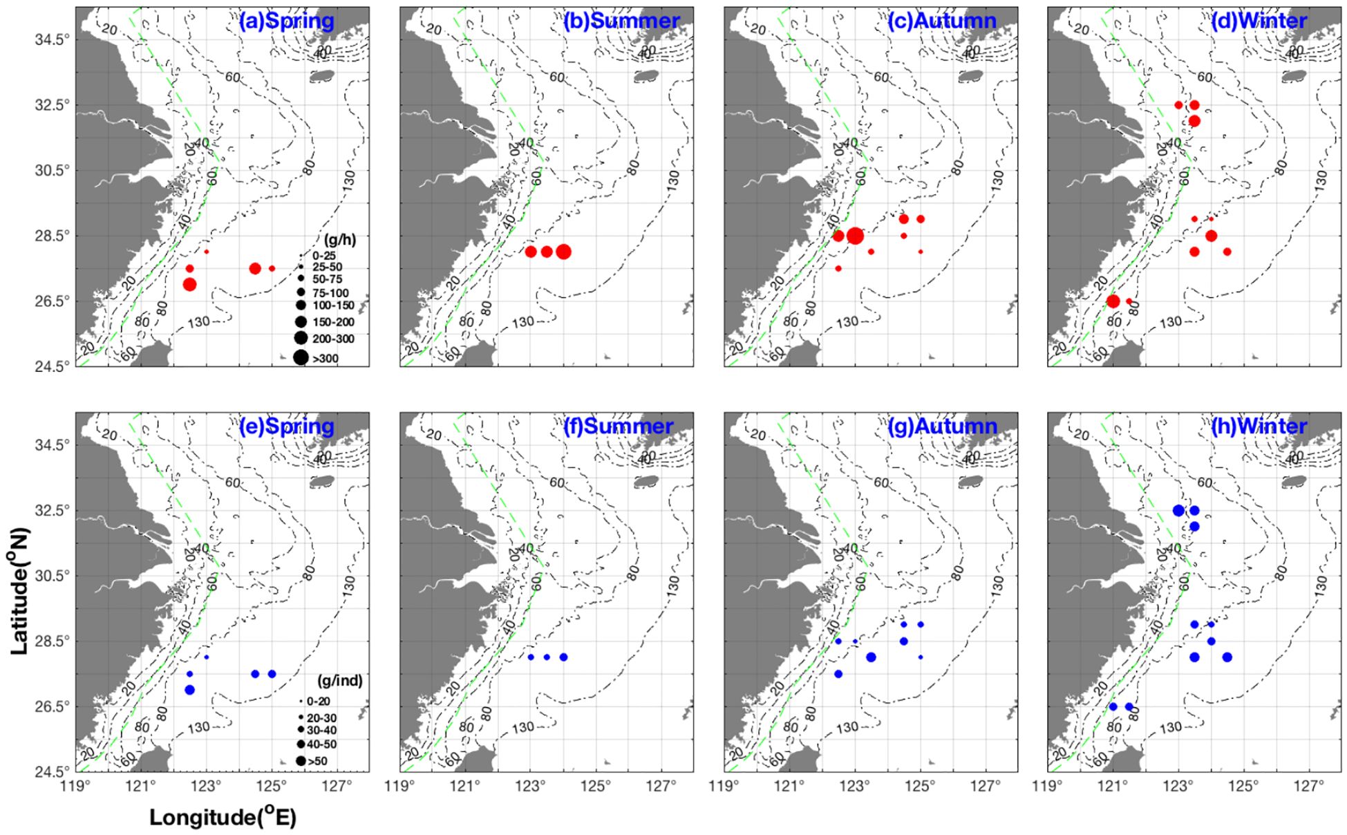
Figure 2. Seasonal distribution characteristics of CPUE_w (unit: g h^–1), shown in red (grouped into 0–25, 25–50, 50–75, 75–100, 100–150, 150–200, 200–300, and > 300 g h^–1) and AIW (unit: g ind^–1) shown in blue (grouped into 0–20, 20–30, 30–40, 40–50, and > 50 g ind^–1) for AmphiOctopus ovulum. The values are represented by circle size. CPUE_w in (a) spring, (b) summer, (c) autumn, (d) winter; AIW in (e) spring, (f) summer, (g) autumn, (h) winter.

Table 1

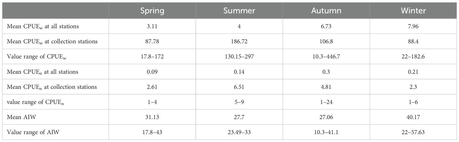
Table 1. Seasonal data for catch per unit effort by weight (CPUE_w) and by number (CPUE_n) and average individual weight (AIW) for AmphiOctopus ovulum from spring to winter.

The measured SBT and SBS value ranges were 10.81–27.06°C and 31.73–35.25‰ respectively (Table 2), and in a case of CPUEn = 24 ind·h−1 the measured SBT and SBS values were 21.33°C and 34.40‰, respectively, in autumn (Figure 3). The value range of the maximum depth at which A. ovulum was found from spring to winter was 91.00–103.00 m (Table 2), indicating the offshore distribution patterns of A. ovulum from spring to autumn. In contrast, the lower limit value of depth for A. ovulum in winter was 33.00 m (Table 2), indicating their inshore distribution at this time.

Table 2

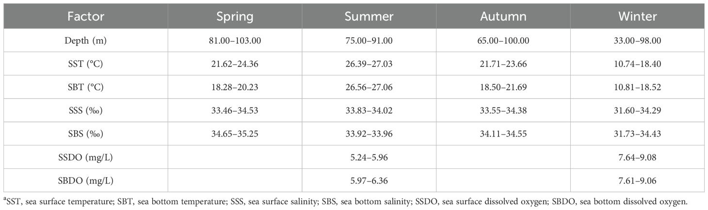
Table 2. Seasonal in situ ranges of environmental variables in the study area^a.

Figure 3

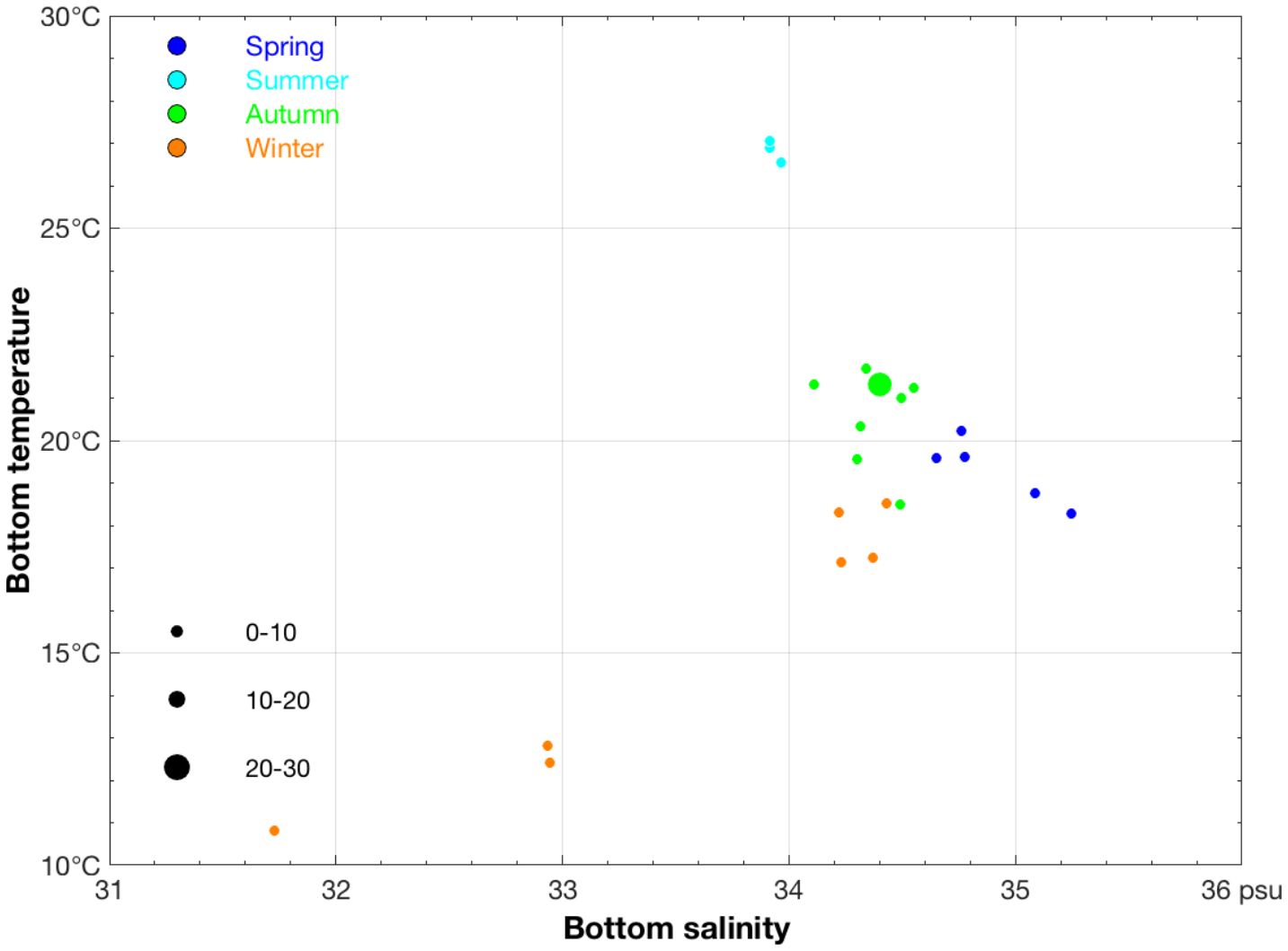
Figure 3. Relationship between sea bottom salinity (unit: ‰) and sea bottom temperature (unit: °C) for CPUE_n sizes classified by group (0–10, 10–20, and 20–30 ind/h) of the species AmphiOctopus ovulum. The data for spring, summer, autumn, and winter are denoted by blue, light sky blue, green, and brown-red solid circles, respectively.

The measured SST value range of A. ovulum was similar in spring and autumn and showed a characteristically narrow range (Table 2). The SST and SBT value ranges were similar in summer and winter, while the SST value was 3.00–4.00°C higher than the SBT in spring and autumn (Table 2). The SSS value ranges were 33.46–34.53‰ in spring to autumn (Table 2), showing the species’ seasonal offshore distribution, and the SSS value increased to 31.60–34.29‰ in winter (Table 2), indicating their inshore distribution in winter. The SBS value range was ranked in spring > autumn > summer > winter (Table 2), showing the species offshore distribution pattern in spring, the influences of fresh water river runoff in summer, a more offshore distribution in autumn, and their occurrence in a larger range of SBS values in winter.

In terms of seasonal variations in distribution, A. ovulum were distributed in the Mindong–Wentai–Yushan fishing grounds in spring, before moving further north to the Zhoushan fishing ground and the offshore areas of the southern East China Sea in the summer, giving rise to a diagonal zone of distribution with its northeastern part in the southern and central East China Sea in autumn, and a winter distribution in the area 26.50°–27.50°N, 122.50°–123.00°E (Figure 4). The current distribution of A. ovulum covers the area 27.50°–28.00°N, 122.50°–123.50°E, but predictions of the effect of global warming on the distribution of their preferred sea temperature suggest probable future range expansion to the northeast and southwest independently (Figure 5a). Under the SSP1-2.6 climate scenario their range would cover 27.00°–29.00°N, 121.50°–125.00°E in 2050 (Figure 5b) and 27.00°–28.50°N, 122.00°–125.00°E in 2100 (Figure 5c). Under the SSP5-8.5 scenario their range would cover 26.50°–29.00° N, 121.00°–125.50° E in 2050 (Figure 5d) and 27.00°–29.00°N, 122.00°–125.50°E in 2100 (Figure 5e).

Figure 4

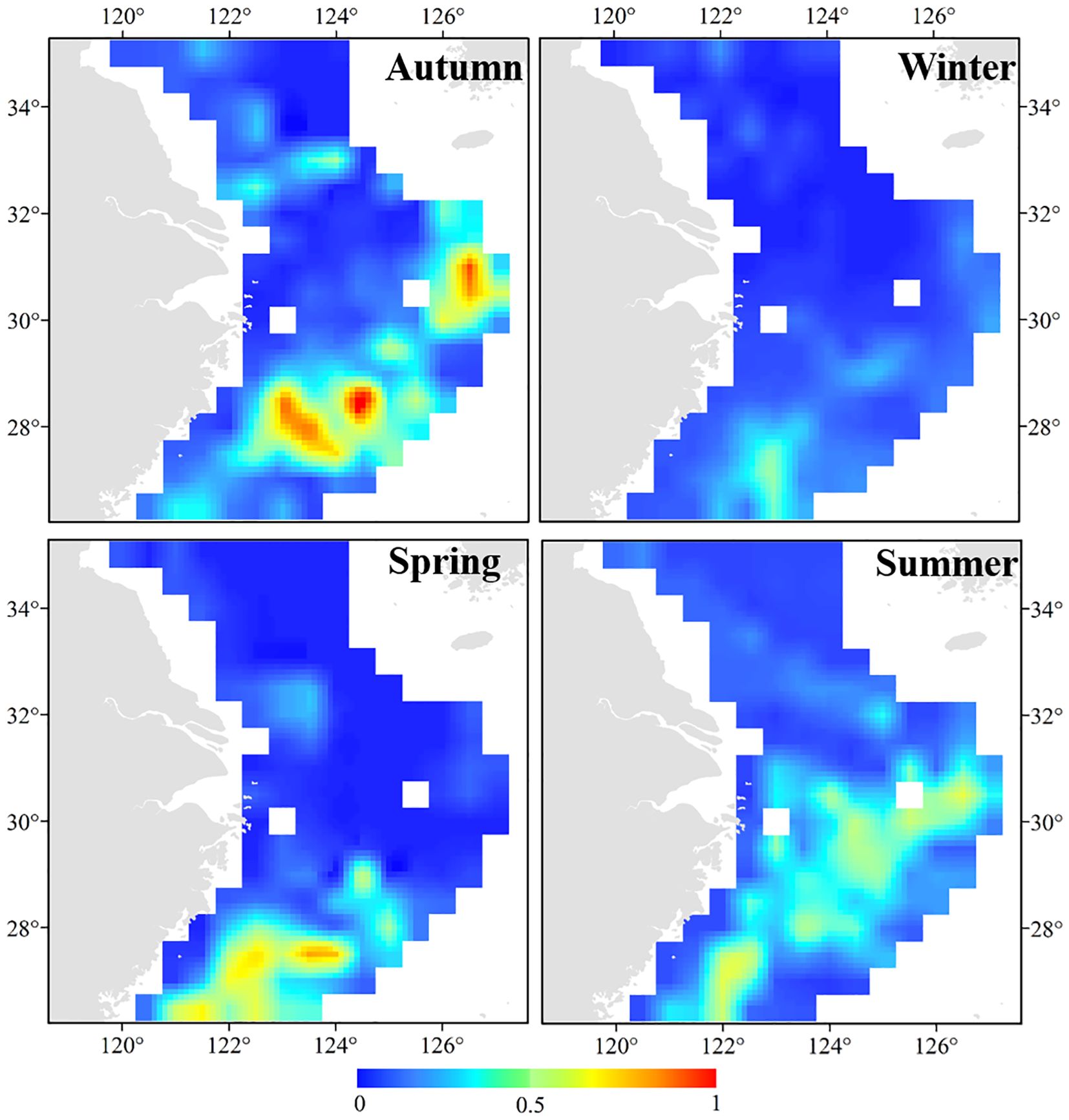
Figure 4. Distribution patterns of AmphiOctopus ovulum in the study area predicted with the random forest and boosted regression trees methods in spring to winter. The bar colored in blue to red indicates the range from low (=0) to high (=1) suitability.

Figure 5

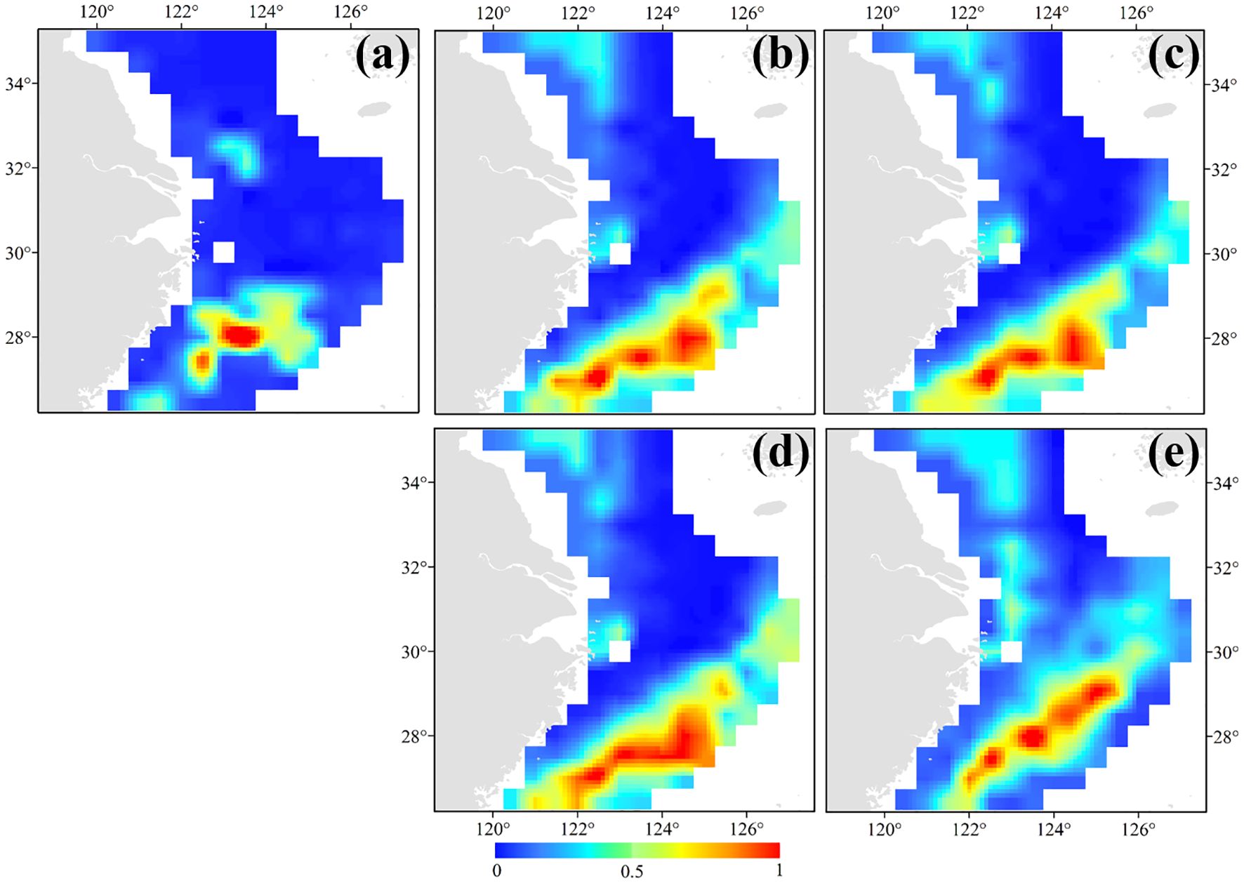
Figure 5. Habitat distribution patterns of AmphiOctopus ovulum in the cases of (a) annual mean habitat; (b) SSP1-2.6 in 2050; (c) SSP1-2.6 in 2100; (d) SSP5-8.5 in 2050; and (e) SSP5-8.5 in 2100. The bar colored in blue to red indicates the range from low (=0) to high (=1) suitability.

4 Discussion

AmphiOctopus ovulum (Sasaki 1917) is a species of small to moderate size. Kubodera and Lu (2002) have confirmed that A. ovulum is distributed from the South China Sea to the waters around the Okinawa Islands and western Japan (Kubodera and Lu, 2002). This species was first reported as Polypus ovulum, and the first review of its taxonomy was reported by Sasaki (1929).

In terms of biomass and number, a survey indicated a mean CPUEw order of Sepia esculenta > Sepia kobiensis > Sepiella maindroni > Loliolus beka > A. ovulum > Loliolus uyii in spring; S. esculenta > S. maindroni > S. kobiensis > A. ovulum > L. uyii > L. beka in summer; S. esculenta > L. beka > S. maindroni > S. kobiensis > L. uyii > A. ovulum in autumn; and S. esculenta > S. maindroni > S. kobiensis > L. beka > A. ovulum > L. uyii in winter (Dou, 2017; Pang et al., 2020; Liang et al., 2025). The mean CPUEn order was S. kobiensis > L. beka > L. uyii > S. esculenta > S. maindroni > A. ovulum in spring; S. esculenta > S. maindroni > S. kobiensis > L. uyii > A. ovulum > L. beka in summer; L. beka > S. kobiensis > L. uyii > S. esculenta > A. ovulum > S. maindroni in autumn; and L. beka > S. kobiensis > L. uyii > S. maindroni > A. ovulum > S. esculenta in winter (Xu et al., 2024a; Xu et al., 2024b; Xu et al., 2024c).

With the intensification of CO2 emissions, Xu et al. (2024a), Xu et al. (2024b), Xu et al. (2024c) and Yang et al. (2025) argued that the habitat of Sepiella maindroni would shift to the south first and then to the north, and it would first expand and then greatly decrease; the habitat area of Sepia kobiensis would be decreasing; the habitat area of A. fangsiao will shrink significantly; Octopus variabilis will shift northward offshore (Pang et al., 2020; Yang et al., 2025). This study has some limitations. Specifically, the methods used in this study have potential risk of overfitting in predicting future distributions of both species under different climate scenarios (Torrejón-Magallanes et al., 2021). In the future, greater understanding of early life history traits, migration routes, and the variations in number and biomass corresponding to changes in environmental variables will be necessary to better protect species stocks.

The main results of our study can be summarized as follows:

1. AmphiOctopus ovulum is distributed in the area 27.00°–29.00°N, 122.50°–125.00°E in spring to autumn, and expands to the area 26.50°–32.50°N, 121.00°–124.50°E in winter.

2. The measured sea bottom temperature and sea bottom salinity values indicate the species offshore distribution pattern in spring, the influences of fresh water river runoff in summer, a more offshore distribution in autumn, and the occurrence in a larger varying environmental range in winter.

3. The core habitat of A. ovulum is in the area 27.50°–28.00°N, 122.50°–123.50°E, and this area would expand to the northeast and southwest independently in the future under the influence of global warming.

Data availability statement

The original contributions presented in the study are included in the article/supplementary material. Further inquiries can be directed to the corresponding author.

Ethics statement

Ethical approval was not required for the study involving animals in accordance with the local legislation and institutional requirements because the species is a common species. We don’t need ethical approval in China.

Author contributions

LY: Methodology, Visualization, Writing – original draft, Writing – review & editing. MX: Investigation, Methodology, Writing – original draft, Writing – review & editing. YC: Investigation, Methodology, Writing – review & editing. SL: Writing – review & editing, Methodology.

Funding

The author(s) declare that financial support was received for the research and/or publication of this article. This research was supported by the National Key R&D Program of China (Grant/Award Numbers: 2024YFD2400404).

Acknowledgments

The authors wish to thank the crews of the fishing boats for their help with field sampling; members of the Key Laboratory of East China Sea and the Oceanic Fishery Resources Exploitation, Ministry of Agriculture and Rural Affairs; and Wenquan Sheng for constructive discussions and encouragement.

Conflict of interest

The authors declare that the research was conducted in the absence of any commercial or financial relationships that could be construed as a potential conflict of interest.

Generative AI statement

The author(s) declare that no Generative AI was used in the creation of this manuscript.

Publisher’s note

All claims expressed in this article are solely those of the authors and do not necessarily represent those of their affiliated organizations, or those of the publisher, the editors and the reviewers. Any product that may be evaluated in this article, or claim that may be made by its manufacturer, is not guaranteed or endorsed by the publisher.

References

Beyer R., Krapp M., Manica A. (2000). An empirical evaluation of bias correction methods for palaeoclimate simulations. Clim. Past 16, 1493–1508. doi: 10.5194/cp-16-1493-2020

Crossref Full Text | Google Scholar

Checkley D. M., Asch R. G., Rykaczewski R. R. (2017). Climate, anchovy, and sardine. Annu. Rev. Mar. Sci. 9, 469–493. doi: 10.1146/annurev-marine-122414-033819

PubMed Abstract | Crossref Full Text | Google Scholar

Dou C. F. (2017). Analysis of genetic diversity and structure of Octopus ovulum. China Water Transport 17, 165–167.

Google Scholar

FAO (2024). The state of world fisheries and aquaculture 2024 – Blue transformation in action (Rome: Food and Agriculture Organization of the United Nations).

Google Scholar

IPCC (Intergov. Panel Clim. Change) (2013). Summary for policymakers. In Climate Change 2013: The Physical Science Basis. Contribution of Working Group I to the Fifth Assessment Report of the Intergovernmental Panel on Climate Change. Eds. Stocker T. F., Qin D., Plattner G. K., Tignor M., Allen S. K., et al (Cambridge, UK: Cambridge Univ. Press), 1–30.

Google Scholar

Keeling R. (2016). The Keeling curve (San Diego: Univ. Calif.). Available online at: https://scripps.ucsd.edu/programs/keelingcurve (Accessed October 24, 2024).

Google Scholar

Kubodera T., Lu C. C. A. (2002). review of cephalopod fauna in Chinese–Japanese subtropical region. Natl. Sci. Museum Monogr. 22, 159–171.

Google Scholar

Le Quere C. (2010). Trends in the land and ocean carbon uptake. Envir. Sustain 2, 219–224. doi: 10.1016/j.cosust.2010.06.003

Crossref Full Text | Google Scholar

Li S. F., Yan L. P., Li H. Y., Li J. S., Cheng J. H. (2006). Spatial distribution of cephalopod assemblages in the region of the East China Sea. J. Fishery Sci. China 13, 936–944.

Google Scholar

Liang J., Zhou Y., Wu T., Chen F., Xu K., Fang G., et al. (2025). Spatiotemporal distribution patterns of cephalopods and their responses to changes in the marine environment in the coastal waters of Zhejiang, China. Front. Mar. Sci. 12, 1510574. doi: 10.3389/fmars.2025.1510574

Crossref Full Text | Google Scholar

Liu S., Liu Y., Teschke K., Hindell M. A., Downey R., Woods B., et al. (2024a). Incorporating mesopelagic fish into the evaluation of conservation areas for marine living resources under climate change scenarios. Mar. Life. Sci. Tech 6, 68–83. doi: 10.1007/s42995-023-00188-9

PubMed Abstract | Crossref Full Text | Google Scholar

Liu S., Liu Y., Xing Q., Li Y., Tian H., Luo Y., et al. (2024b). Climate change drives fish communities: changing multiple facets of fish biodiversity in the Northwest Pacific Ocean. Sci. Total. Environ. 955, 176854. doi: 10.1016/j.scitotenv.2024.176854

PubMed Abstract | Crossref Full Text | Google Scholar

Liu S., Tian Y., Liu Y., Alabia I. D., Cheng J., Ito S. (2023). Development of a prey-predator species distribution model for a large piscivorous fish: a case study for Japanese spanish mackerel Scomberomorus niphonius and Japanese anchovy Engraulis japonicus. Deep. Sea. Res. Part. II 207, 105227. doi: 10.1016/j.dsr2.2022.105227

Crossref Full Text | Google Scholar

Ottersen G., Kim S., Huse G., Polovina J. J., Stenseth N. C. (2010). Major pathways by which climate may force marine fish populations. J. Mar. Syst. 79, 343–360. doi: 10.1016/j.jmarsys.2008.12.013

Crossref Full Text | Google Scholar

Pang Y. M., Tian Y. J., Fu C. H., Ren Y. P., Wan R. (2020). Growth and distribution of amphioctopus fangsiao (d’Orbigny, 1839-1841) in Haizhou Bay, Yellow Sea. J. Ocean Univ. China 19, 1125–1132. doi: 10.1007/s11802-020-4322-7

Crossref Full Text | Google Scholar

Qin T., Yu C., Chen Q., Ning P., Zheng J. (2011). Species composition and quantitative distribution study on cephalopod in the Zhoushan fishing ground and adjacent waters. Oceanol. Limnlo. Sin. 42, 124–130.

Google Scholar

Räty O., Räisänen J., Ylhäisi J. S. (2014). Evaluation of delta change and bias correction methods for future daily precipitation: intermodel cross-validation using ENSEMBLES simulations. Clim. Dyn 42, 2287–2303. doi: 10.1007/s00382-014-2130-8

Crossref Full Text | Google Scholar

Riahi K., Van Vuuren D. P., Kriegler E., Edmonds J., O’Neill B. C., Fujimori S., et al. (2017). The shared socioeconomic pathways and their energy, land use, and greenhouse gas emissions implications: an overview. GEC 42, 153–168. doi: 10.1016/j.gloenvcha.2016.05.009

Crossref Full Text | Google Scholar

Rosa R., Pissarra V., Borges F. O., Xavier J., Gleadall I. G., Golikov A., et al. (2019). Global patterns of species richness in coastal cephalopods. Front. Mar. Sci. 6, 469. doi: 10.3389/fmars.2019.00469

Crossref Full Text | Google Scholar

Sasaki M. (1929). A monograph of the dibranchiate cephalopods of the Japanese and adjacent waters. J. Faculty Agriculture Hokkaido Imperial Univ. 20, 55–58.

Google Scholar

Torrejón-Magallanes J., Ángeles-González L. E., Csirke J., Bouchon M., Morales-Bojórquez E., Arreguín-Sánchez F. (2021). Modeling the Pacific chub mackerel (Scomber japonicus) ecological niche and future scenarios in the northern Peruvian Current System. Prog. Oceanogr. 197, 102672. doi: 10.1016/j.pocean.2021.102672

Crossref Full Text | Google Scholar

Xu M., Feng W., Liu Z., Li Z., Song X., Zhang H., et al. (2024a). Seasonal-spatial distribution variations and predictions of Loliolus beka and Loliolus uyii in the East China Sea region: implications from climate change scenarios. Animals 14, 2070. doi: 10.3390/ani14142070

PubMed Abstract | Crossref Full Text | Google Scholar

Xu M., Liu S., Zhang H., Li Z., Song X., Yang L., et al. (2024b). Seasonal analysis of spatial distribution patterns and characteristics of Sepiella maindroni and Sepia kobiensis in the East China Sea region. Animals 14, 2716. doi: 10.3390/ani14182716

PubMed Abstract | Crossref Full Text | Google Scholar

Xu M., Wang Y., Liu Z., Liu Y., Zhang Y., Yang L., et al. (2023). Seasonal distribution of the early life stages of the small yellow croaker (Larimichthys polyactis) and its dynamic controls adjacent to the Changjiang river estuary. Fish. Oceanogr. 32, 390–404. doi: 10.1111/fog.12635

Crossref Full Text | Google Scholar

Xu M., Yang L., Liu Z., Zhang Y., Zhang H. (2024c). Seasonal and spatial distribution characteristics of Sepia esculenta in the East China Sea region: transfer of the central distribution from 29° N to 28° N. Animals 14, 1412. doi: 10.3390/ani14101412

PubMed Abstract | Crossref Full Text | Google Scholar

Yang L. L., Xu M., Liu Z., Zhang Y., Cui Y., Li S. (2025). Seasonal and spatial distribution of AmphiOctopus fangsiao and Octopus variabilis in the southern Yellow and East China Seas: Fisheries management implications based on climate scenario predictions. Regional Stud. Mar. Sci. 83, 104072. doi: 10.1016/j.rsma.2025.104072

Crossref Full Text | Google Scholar

Zhu Y., Lin Y., Chu J., Kang B., Reygondeau G., Zhao Q., et al. (2022). Modelling the variation of demersal fish distribution in Yellow Sea under climate change. J. Ocean. Limnol. 40, 1544–1555. doi: 10.1007/s00343-021-1126-6

Crossref Full Text | Google Scholar

Zhu W. B., Xue L. J., Lu Z. H., Xu H. X., Xu K. D. (2014). Cephalopod community structure and its relationship with environmental factors in the southern East China Sea. Oceanol. Limnlo. Sin. 45, 436–442.

Google Scholar