Boundary currents in the Bransfield Strait: near-surface interbasin water volume and heat exchange

The Bransfield Strait, located between the Bellingshausen and Weddell seas, serves as a natural laboratory for studying boundary current dynamics and interbasin exchange in polar regions of the world ocean. Using 30 years (1993–2022) of multi-platform satellite data (altimetry, sea surface temperature, air temperature, sea ice coverage, and wind stress), this study examines the near-surface spatiotemporal variability of the Bransfield Current and Antarctic Coastal Current. The Bransfield Current consistently strengthens up to King George Island across all seasons, with volume transport (0-100 m depth) increasing from 0.24–0.33 Sv in the western transect to 0.52–0.64 Sv in the eastern transect in the Bransfield Strait, exhibiting limited seasonal variability, while decreasing downstream as it recirculates around the SSI. In contrast, the Antarctic Coastal Current displays pronounced seasonality, with volume transport oscillating between 0.19–0.38 Sv in the western transect and 0.05–0.33 Sv in the eastern transect in the Bransfield Strait. Heat transport analyses reveal significant asymmetries: the Bransfield Current contributes up to 5.44x10¹² W eastward in summer based on a hydrographic climatology constructed from CTD, MEOP, and Argo float measurements (0–100 m depth) and 6.67x10¹¹ W using remotely-sensed sea surface temperature (0–10 m depth). Complementary to this, while smaller in magnitude, the Antarctic Coastal Current peaks at 2.13x10¹² W (0–100 m depth) and 2.67x10¹¹ W (0–10 m depth) westward in summer, respectively. Notably, the net heat transport balance approaches zero during winter, likely reflecting periods of reduced interbasin heat exchange driven by homogeneous temperatures and sea ice coverage. Seasonal shifts in near-surface volume and heat balances, driven by wind stress and temperature gradients, highlight the critical role of these boundary currents in shaping local hydrography and sea ice dynamics. Lastly, the evaluation of two global ocean reanalysis products (GLORYS12V1 and HYCOM) reveals their inability to accurately represent the Bransfield Strait circulation, emphasizing the need for high-resolution observational data and improved models to better resolve boundary current dynamics. These findings establish a comprehensive baseline for assessing climate-driven changes in the near-surface layers of the boundary currents that exchange water masses with distinct properties between basins in the Antarctic Peninsula region.

1 Introduction

The west Antarctic Peninsula is particularly sensitive to climate change due to the profound implications that varying warm/cold water pathways have for glacier dynamics and sea ice cover in this region (Cook et al., 2016). In this setting, the Bransfield Strait (BS), located between the Antarctic Peninsula (AP) and the South Shetland Islands (SSI), acts as a gateway and a key region for water masses exchange between the Bellingshausen and Weddell seas; two sea basins which differ markedly in their thermohaline properties. In addition, the BS can be divided into three distinct basins: the western, central, and eastern basins (WB, CB, and EB, respectively, in Figure 1; Gordon and Nowlin, 1978; López et al., 1999), which are separated by sills with depths of 630 m (WB-CB) and 1000 m (CB-EB).

Figure 1

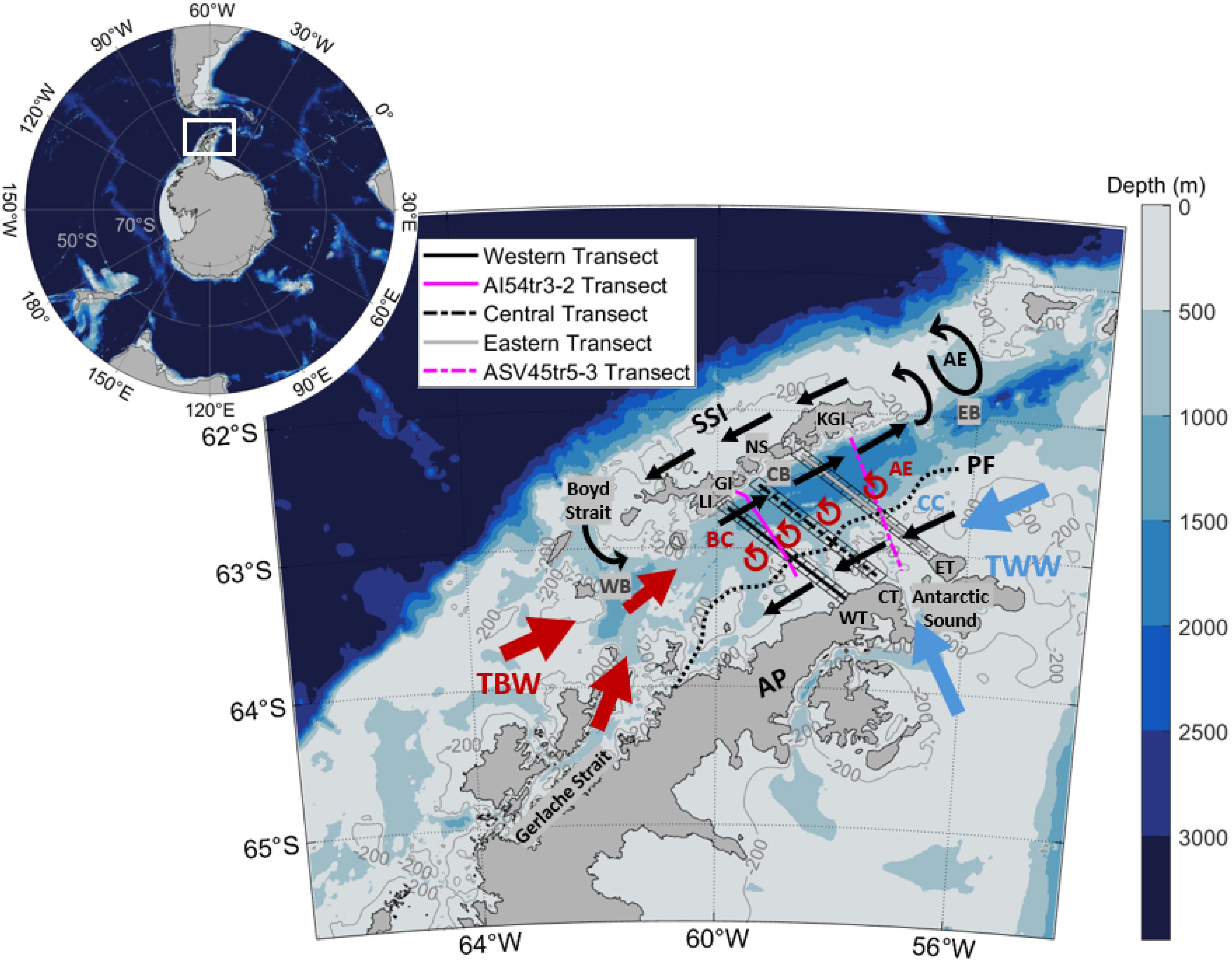
Figure 1. Sketch of the circulation in the Bransfield Strait with indication to key geographical locations and oceanographic features. Acronyms for the South Shetland Islands (SSI) include LI (Livingston Island), GI (Greenwich Island), and KGI (King George Island). Acronyms for the western, central, and eastern basins (WB, CB, and EB, respectively) as well as for Nelson Strait (NS) and Antarctic Peninsula (AP) are also shown. Acronyms for major oceanographic features are as follows: AE (anticyclonic eddy), BC (Bransfield Current), CC (Antarctic Coastal Current), PF (Peninsula Front), TBW (Transitional Bellingshausen Water) and TWW (Transitional Weddell Water). Additionally, five transects are shown (see the legend for line styles and color coding). Three of these—Western Transect (WT), Central Transect (CT), and Eastern Transect (ET)—are defined according to Veny et al. (2022) and are used in this study to capture spatio-temporal variability of atmospheric and oceanic properties. The other two are cruise transects from Frey et al. (2023): one conducted on 24 November 2017 from the Antarctic Peninsula to Livingston Island by the R/V Akademik Ioffe (AI), labeled as code 54tr3_2, and another on 18–19 December 2017 from the Antarctic Sound to King George Island by the R/V Akademik Sergey Vavilov (ASV), labeled as code 45tr5_3.

At surface, the BS is characterized by the convergence of two distinct water masses: the relatively warm, less saline waters of the Bellingshausen Sea typically found within the first 300 m (Transitional Bellingshausen Water, TBW: θ > -0.4°C, salinity < 34.35, and density σ_θ < 27.64 kg m⁻³; Sangrà et al., 2017) and the colder, more saline waters of the Weddell Sea distributed throughout the water column (Transitional Weddell Water, TWW: θ < -0.4°C, salinity > 34.35, and density σ_θ > 27.64 kg m⁻³; Sangrà et al., 2017). These water masses are transported, respectively, by the following primary currents: the Bransfield Current (BC), which flows northeastward throughout the basins as a baroclinic narrow jet along the SSI, and recirculates counterclockwise to the north of the islands (Sangrà et al., 2017), and the Antarctic Coastal Current (CC), a wide, slow-moving current that extends to deeper waters and flows southwestward along the AP slope (Figure 1). Following this scenario, the BS serves as a natural laboratory for studying the complex interactions between oceanic boundary currents transporting relatively warm and cold water masses.

The BC and CC jointly form a cyclonic-like circulation within the strait, with a street of mesoscale anticyclonic eddies of TBW characteristics in between (Sangrà et al., 2011, 2017), where the Peninsula Front (PF) serves as a seasonal hydrographic boundary. The PF is formed by a sharp gradient between TBW and TWW, and responds to the variability of boundary currents and the water mass exchange they drive. During the austral summer, the PF is well defined due to the heightened contrast between the warmer and fresher TBW and the colder and saltier TWW (García et al., 1994; López et al., 1999; Sangrà et al., 2017), while in winter, the front dissipates as the thermal gradient weakens due to the cooling and deepening of surface waters, which homogenizes the water column (Veny et al., 2024). The variations of the PF location and strength are thus essential for understanding the horizontal and vertical distribution of water masses (García-Muñoz et al., 2013; Sangrà et al., 2017; Gordey et al., 2024).

Year-to-year variability in the BC and CC further influences oceanic forcing on glacier and sea-ice dynamics in the BS and farther south (Cook et al., 2016; Vorrath et al., 2020, 2023), with changes in sea-ice extent and duration having cascading effects on local climate, ocean circulation, and ecosystem productivity (Schofield et al., 2010; Ducklow et al., 2013; Eayrs et al., 2019).

Lastly, the PF and boundary currents in the BS also play a critical role in shaping phytoplankton niches and, consequently, the entire marine food web and governing biogeochemical processes (Loeb et al., 1997; Montes-Hugo et al., 2009; García-Muñoz et al., 2013; Veny et al., 2024). During the austral summer, surface chlorophyll-a concentrations are elevated near the SSI, while near the AP the phytoplankton blooms seem to develop less abruptly and at deeper levels (Veny et al., 2024). This biophysical interaction between ocean circulation, fronts and primary productivity sustains local and remote Antarctic marine ecosystems (Loeb et al., 1997, 2009; Atkinson et al., 2004; Johnston et al., 2022; Annasawmy et al., 2023), including Antarctic krill (Euphausia superba), a key species in this ecosystem (Murzina et al., 2023).

Building on previous studies, we aim to provide new insights into the seasonal interplay between boundary currents, atmospheric forcing, oceanic forcing, and sea ice dynamics governing the circulation in the BS. We expect our results will serve as a baseline for future research on long-term trends in the west AP ocean circulation and sea ice dynamics. Additionally, they will help to understand how Antarctic marine ecosystems respond to climate variability, given that local boundary currents and hydrography shape the phytoplankton bloom phenology and structure (Veny et al., 2024).

The manuscript is organized as follows. In Section 2, we describe the data and methods used in our study. In Section 3, we present and discuss the results. First, in Section 3.1, we analyze the surface geostrophic velocities of the boundary currents: BC and CC. Second, in Section 3.2, we examine their oceanic and atmospheric forces, including Sea Surface Temperature (SST), air temperature, and Sea Ice Coverage (SIC). In addition, in Section 3.3, we evaluate the wind stress and its correlation with the surface geostrophic velocities to assess this atmospheric forcing on the boundary currents. In Section 3.4, we characterize the monthly climatology of near-surface volume and heat transport of the boundary currents and their balances using altimeter-derived surface geostrophic seawater velocity, temperatures from Dotto et al. (2021), and remotely-sensed SST. Section 4 concludes with a summary of main findings. Finally, in Appendix, we discuss the limitations of surface drifter data and two open-access global ocean reanalysis products, and emphasize the need for improved models and high-resolution data integration.

2 Data and methods

This section outlines the data sources and methodologies. The satellite datasets described below cover the period from 1993 to 2022 (30 years), providing a comprehensive foundation for evaluating the boundary currents in the BS. The climatological Shipboard Acoustic Doppler Current Profiler (SADCP) data from Veny et al. (2022) cover the years 1999 to 2014. We also use synoptic data collected in 2017, firstly analysed, and made available, by Frey et al. (2023). The seasonal climatological temperature fields, derived from Conductivity, Temperature and Depth (CTD), Marine Mammals Exploring the Oceans Pole to Pole (MEOP), and Argo float measurements as described by Dotto et al. (2021), cover the period from 1990 to 2019. The in situ drifter data and reanalysis products, addressed in the Appendix, span the periods 1979 to the present and 1994–2015, respectively.

2.1 Satellite data: altimeter-derived surface currents, SST, SIC, air temperature, wind stress

We use altimeter-derived surface geostrophic eastward and northward sea water velocity processed by the Data Unification Altimeter Combination System (DUACS) multimission altimeter data processing system. For detailed spatial and temporal analyses, the dataset employed corresponds to a processing Level 4 (L4), encompassing a global ocean coverage with a spatial resolution of 0.25°×0.25°. The data availability spans from January 1993 to September 2023 (https://doi.org/10.48670/moi-00148). To analyze the structure of the boundary currents as they flow parallel to the main axis of the BS, aligned with the southern slope of the SSI and the western slope of the AP, the cartesian coordinate system is rotated counterclockwise. We refer, hereafter, to the rotated reference system as: along the strait ($x\text{'}$) and across the strait ($y\text{'}$). This rotation angle, 36.25°, corresponds to the average orientation of the across-strait grid cells shown in Veny et al. (2022). In each transect, the eastward and northward altimeter-derived surface velocity components are transformed to derive the along-strait ($u\text{'}$) and across-strait ($v\text{'}$) velocities.

SST and SIC data originate from the Operational Sea Surface Temperature and Ice Analysis (OSTIA; Good et al., 2020), developed by the United Kingdom Met Office. These datasets were obtained from the Copernicus Marine Environment Monitoring Service (CMEMS; https://marine.copernicus.eu/). OSTIA provides SST data corrected for diurnal variability and includes information on sea ice coverage. This dataset is the result of reprocessing, combining both in situ and satellite data, and provides a grid resolution of 0.05°x0.05° (https://doi.org/10.48670/moi-00168). It is categorized as a L4 processing product and covers a temporal range from October 1981 to May 2022. The choice of this product is based on its alignment with in situ measurements, as reported in Veny et al. (2024). The time-series of daily SST and SIC up to May 2022 is extended from June 2022 to December 2022 using the near-real time product from OSTIA (https://doi.org/10.48670/moi-00165). Besides providing climatological fields of SST and SIC, the OSTIA product is also used to compute heat transport (see Section 2.4).

The atmospheric forcing is addressed using monthly averaged reanalysis data of wind components at 10 m and air temperature at 2 m from ERA5 (Hersbach et al., 2020), which features a horizontal resolution of 0.25°x0.25°. Subsequently, the along- (${\tau }_{x\text{'}}$) and across-strait (${\tau }_{y\text{'}}$) wind stress components (Equation 1) are computed as follows:

$\begin{array}{ll}{\tau }_{x\text{'}} =u\text{'} · \rho · U{\text{'}}_{10}· C_D ; {\tau }_{y\text{'}}=v\text{'} · \rho · U{\text{'}}_{10}· C_D& (1)\end{array}$

where $u\text{'}$ and $v\text{'}$ are the eastward and northward velocity components after being rotated 36.25° counterclockwise according to the strait orientation; $\rho$ is the air density (1.2 kg m^-3); $U{\text{'}}_{10}=\sqrt{u{\text{'}}^2+v{\text{'}}^2}$ is the wind speed at 10 m above the surface; and, $C_D$ is the drag coefficient, which is a function of wind speed, $U{\text{'}}_{10}$, taking into account sea ice cover, as described by Lüpkes and Birnbaum (2005).

2.2 In situ data: SADCP, temperature at depth and surface drifters

We use publicly available in situ velocity data, collected from SADCPs, for intercomparison with the satellite-based seasonal climatologies presented in this work. Velocity measurements were rotated following the same procedure as for altimeter-derived surface velocities.

The analysis relies on two extensive datasets of direct velocity measurements collected from 1999 to 2014 with 150 kHz ‘narrow band’ SADCPs along ship tracks from R/V Nathaniel B. Palmer and R/V Laurence M. Gould, which navigated routinely from South America to Antarctica for logistical operations during all the seasons. Data acquisition and initial processing were accomplished by Dr. Eric Firing (University of Hawaii) and Dr. Teresa Chereskin (Scripps Institution of Oceanography). Velocity profiles were acquired and processed with UHDAS (University of Hawaii Data Acquisition System) and CODAS (Common Ocean Data Access System), respectively. The processed 5 min averaged transect data we use in this work can be found at the Joint Archive for SADCP (JASADCP) webpage, https://uhslc.soest.hawaii.edu/sadcp/. For processing details the reader is referred to Lenn et al. (2007) and Firing et al. (2012). Profiles collected from R/V Nathaniel B. Palmer have a vertical resolution of 8 m from 31 to 503 m depth, while profiles collected from R/V Laurence M. Gould have a vertical resolution of 10 m from 30 to 1040 m depth. We address vertical interpolation on standard depth levels through both datasets towards a common 10 m vertical resolution starting at 30 m depth. Before gridding the data, the barotropic tidal signal was removed using the Circum-Antarctic Tidal Simulation (CATS2008), an update to the model described by Padman et al. (2002). Then, seasonal climatologies of the BC were constructed (Veny et al., 2022). We inspect the SADCP-based seasonal climatologies further in this work for intercomparison with satellite-based climatologies. Lacking enough in situ measurements over the domain of the CC, we address this knowledge gap by using synoptic SADCP data (https://data.mendeley.com/datasets/g58z4mczs7/1) collected by the R/V Akademik Ioffe (AI) and R/V Akademik Sergey Vavilov (ASV) in 2017 (Frey et al., 2021a, 2023). These measurements were taken on 24th November 2017 (transect 54tr3_2) and 18-19 December 2017 (transect 45tr5_3), respectively. The transect 54tr3_2 surveyed a section from AP to Livingston Island, while the transect 45tr5_3 surveyed a section from the Antarctic Sound to King George Island.

Seasonal temperature fields derived from the climatology presented in Dotto et al. (2021) (https://zenodo.org/records/4420006) are used to compute heat transport (see Section 2.4). This climatology is constructed using CTD, MEOP and Argo float measurements in the northern AP and adjacent regions from 1990 to 2019. For consistency, we define seasons hereafter following Dotto et al. (2021): summer (January-March), autumn (April-June), winter (July-September) and spring (October-December). The spatial grid resolution is approximately 10 km with profiles linearly interpolated onto 90 depth levels.

Lastly, data from the NOAA Global Drifter Program (GDP) buoys (‘drifters’), available from 1979 to the present, are also analyzed. The data have been processed by the Drifter Data Assembly Center (DAC) at Atlantic Oceanographic and Meteorological Laboratory (AOML), applying optimal interpolation to generate records at 6-hour intervals (Lumpkin and Centurioni, 2010). The data include time, positions (latitude and longitude), SST, and surface velocities (eastward and northward components). The surface drifter data are analyzed in the Appendix to assess the feasibility of producing seasonal climatological fields that provide an overview of the ocean circulation in the BS, incorporating both boundary currents and direct measurement-based data, given the lack of SADCP measurements covering the entire strait, which prevents a complete depiction of strait-wide circulation. Before starting to process the drifter data, the barotropic tidal signal was also removed using CATS2008, as was done for the SADCP data. The data was then gridded into cells with a resolution of 25 km, matching the resolution of the altimetry data shown in Figure 2. To address the irregular spatial and temporal distribution of the data, we applied a step-by-step time-averaging scheme following Veny et al. (2022).

Figure 2

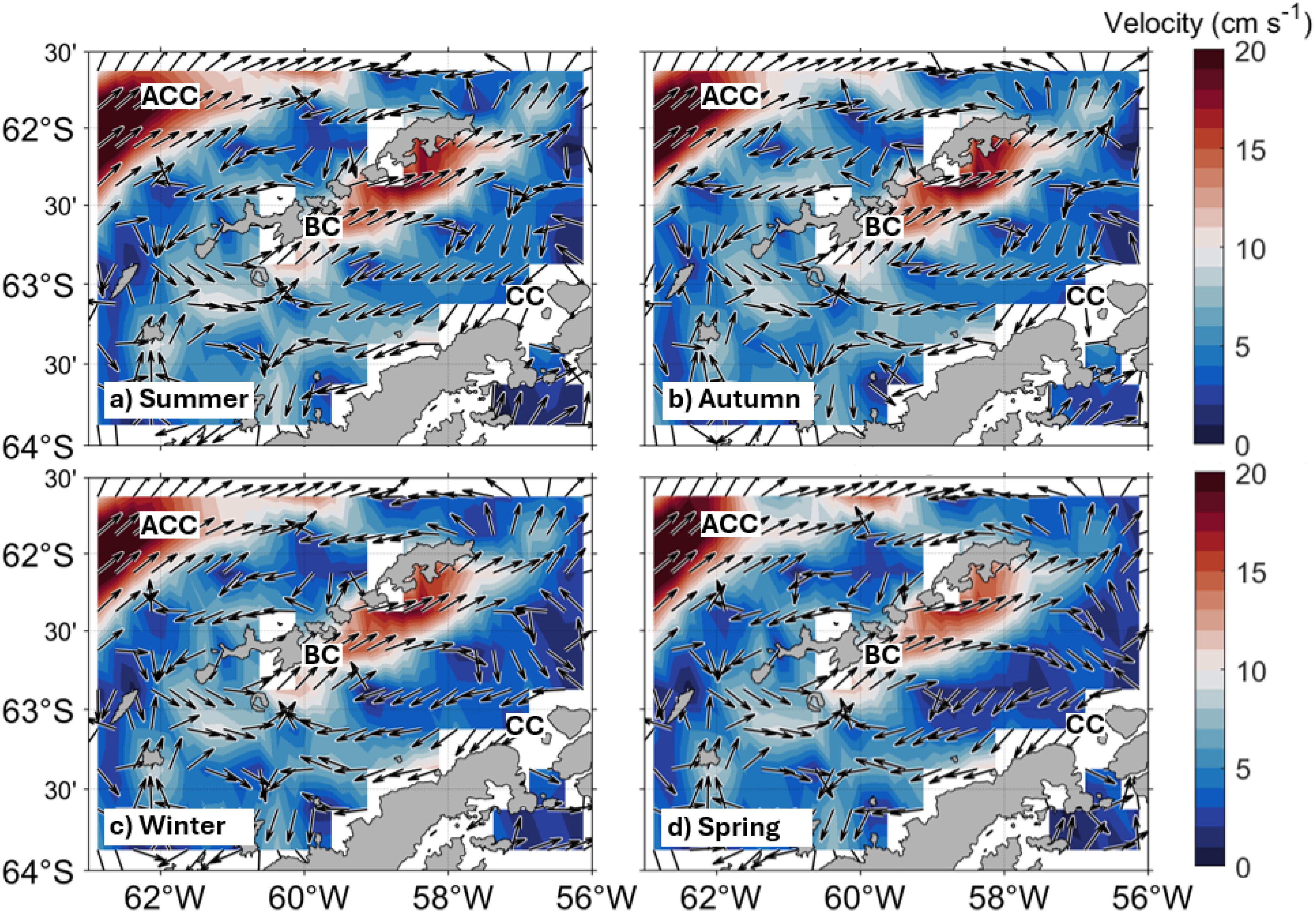
Figure 2. Seasonal surface circulation (shades of colors) from altimeter-derived geostrophic velocities using data from DUACS multimission altimeter data processing system: (a) summer (Jan–Mar), (b) autumn (Apr–Jun), (c) winter (Jul–Sep), and (d) spring (Oct–Dec). The climatologies are seasonally-averaged from January 1993 to December 2022. The vector velocity field is shown as unit vectors, while the magnitude is shown as shades of colors (see colorbar in cm s^-1). The main currents are also indicated: Bransfield Current (BC) and Antarctic Coastal Current (CC), flowing as boundary currents in the Bransfield Strait; and, the Antarctic Circumpolar Current (ACC), north of the South Shetland Islands in the Drake Passage.

2.3 Reanalysis products: sea surface currents

We analyze ocean circulation velocity data from the GLobal Ocean ReanalYsis and Simulation (GLORYS12V1; https://doi.org/10.48670/moi-00021), a global ocean reanalysis product provided by the European Union’s CMEMS. This dataset is generated from coupling ocean-ice models: the version 3.1 of the Nucleus for European Modelling of the Ocean (NEMO) and the version 2 of the Louvain-la-Neuve-Ice Model (LIM2). The common source of atmospheric forcing data is from ERA-Interim. This database covers the period from January 1993 to June 2021 with a horizontal resolution of 1/12° and a vertical resolution of 50 z-levels from surface to 5727.9 m depth. However, our dataset is limited to the period from January 1993 to December 2020 to ensure a consistent number of months for each year.

In addition, we also assess Global Ocean Forecasting System (GOFS) 3.1 output on the GLBv0.08 grid, a version of the global HYCOM-based product (HYbrid Coordinate Ocean Model; https://www.hycom.org/dataserver/gofs-3pt1/reanalysis), from the institution Naval Research Laboratory: Ocean Dynamics and Prediction Branch. The product provides data with 40 vertical levels, a horizontal resolution of 0.08° between 40°S and 40°N, increasing to 0.04° beyond these latitudes, and a temporal resolution of 3 hours, covering the period from 1994 to 2015. The system uses the Navy Coupled Ocean Data Assimilation (NCODA) system, assimilating satellite and in situ sea surface observations, as well as vertical temperature and salinity profiles from XBTs, Argo floats, and moored buoys.

Analogous to the objective pursued with the drifter data, in the Appendix, we aim to complement the analysis of remotely-sensed observations with an analysis of the aforementioned reanalysis products to assess the feasibility of producing seasonal climatological fields that provide an overview of ocean circulation in the BS.

2.4 Estimation of near-surface volume and heat transport

Based on Figure 9 in Frey et al. (2023), we note that assuming barotropicity beyond 100 m would not be a realistic assumption relying solely on satellite data. For this reason, we use the same bottom boundary and focus our analysis in the upper 100 m, where the wind stress forcing and sea-ice formation processes play major roles in the ocean dynamics. The along-strait near-surface volume transport, $U\text{'}$, driven by the boundary currents in the BS from the surface down to 100 m depth (Equation 2) is calculated as follows:

$\begin{array}{ll}U\text{'}(\mathrm{x}\text{'},\mathrm{t}) ={\displaystyle {\text{∫}}_0^{{\mathrm{D}}_{\mathrm{T}}}{\displaystyle {\text{∫}}_h^{h_0}u\text{'} dzdy\text{'}}} & (2)\end{array}$

where $x\text{'}$ is the along-strait coordinate; D_T corresponds to the length of the across-strait transects; the terms h₀ and h refer to the shallowest and deepest depths considered, set at 0 m and 100 m, respectively; and u’ is the along-strait velocity component (in m s^-1) after counterclockwise rotation of 36.25°. To distinguish between the BC and CC domains, we use the 0 cm s^-1 isoline as the boundary of integration along $x\text{'}$. At depth, we use the vertical gradient of the BC velocity profile from Figure 9 in Frey et al. (2023), to accommodate its baroclinic nature for each altimeter-derived surface geostrophic velocity profile. In contrast, for the CC, which has been reported as predominantly a barotropic current, at least during spring and summer (Morozov, 2007; Savidge and Amft, 2009; Poulin et al., 2014; Veny et al., 2022; Frey et al., 2023), the same altimeter-derived surface geostrophic velocity is applied throughout the entire water column (i.e. the integral through depth is omitted and replaced by times the extent of the water column under consideration, which is here 100 m).

The near-surface heat transport, $Q_h$ (Equation 3) is computed as follows:

$\begin{array}{ll}{Q}_h(x\text{'},t) =\rho c_p{\displaystyle {\text{∫}}_0^{D_T}{\displaystyle {\text{∫}}_h^{h_0}u\text{'} (T_i-T_{ref}) dzdy\text{'}}} & (3)\end{array}$

where $x\text{'}$ is the along-strait coordinate; ρ is the seawater density (in kg m^-3), C_p is the specific heat capacity of seawater (in J kg^-1 °C^-1); D_T corresponds to the length of the across-strait transects; the terms h₀ and h refer to the shallowest and deepest depths considered, respectively; $u\text{'}$ is the along-strait velocity component (in m s^-1) after counterclockwise rotation of 36.25°; and T_i - T_ref represents the temperature anomaly at position i with respect to the reference, which is -1.8 (the freezing temperature, in °C). We use two different databases and assumptions regarding the temperature field. First, we allow a vertical variation of the temperature field following the seasonal climatology developed by Dotto et al. (2021), hence using 0 m and 100 m as vertical boundaries. Second, we assume SST is constant within the first 10 m of the water column (i.e. the integral through depth is, in this latter case, omitted and replaced by times the extent of the water column under consideration, which is here 10 m).

3 Results and discussion

3.1 Surface dynamics of the boundary currents

Previous studies have extensively explored the relationship between geostrophic circulation derived from satellite altimetry and direct velocity measurements across various oceanic regions finding a high correlation (Barré et al., 2011; Ferrari et al., 2017; Frey et al., 2021b; Lago et al., 2021). Recently, it has been shown that the mean geostrophic circulation revealed by altimeter-based maps agreed well with the spatial structure of the BC as compared to direct velocity measurements, although the CC was declared not to be clearly represented and, hence, a further description was prevented (Frey et al., 2023). Generally, the comparison between the altimeter-derived surface geostrophic velocity and SADCP measurements showed qualitative coherence, though interpolated altimetry data over the surveys dates always indicated weaker boundary current velocities than in situ observations. Frey et al. (2023) attributed this discrepancy to the unique environmental factors of the region, including small spatial-scale features and the pronounced influence of ocean tides. These tides can drive regional sea level changes of several tens of centimeters (Zhou et al., 2020), while satellite altimetry data rely on tide models to correct such variations. Unfortunately, these tide models exhibit significant inaccuracies in the region (King and Padman, 2005), hence contributing to the observed discrepancies. These limitations compromise the reliability of altimetry-derived geostrophic currents for capturing short-term variability or episodic events in the strait. Overall, Frey et al. (2023) found that BC velocity values in the 0.25° resolution altimetry product were 2.2 times lower than SADCP values when synoptic measurements were compared (i.e. concomitant altimeter-derived velocities and direct velocities measured from SADCPs). Notably, Veny et al. (2022), using climatological velocity fields from SADCP data, reported seasonal variations in the BC, with maximum current speeds during the austral summer. In contrast, Frey et al. (2023), using satellite altimetry data, reported maximum current speeds during austral autumn and minimum speeds (15% lower) in spring. As previously discussed, this mismatch between SADCP and altimetry-derived velocities can likely be attributed to the fact that these datasets represent different ocean layers, which inherently capture distinct dynamics (i.e. SADCP depth-averaged values in Veny et al. (2022) data refer to the 80-100 m depth layer). Additionally, the irregularity of SADCP transects may influence the resulting climatology, and they must be considered as a first-order climatological approximation.

Given that variations in the BC on time scales of several days can be as significant as seasonal variations, a substantially larger SADCP dataset is required to improve the robustness of seasonal variability estimates. For this reason, in this work we focus on the use of satellite altimetry data to assess climatological long-term variations (seasonal scale) in the dominant flows of this dynamic area. We do so by comparison of climatological fields built upon satellite-derived and climatological direct velocities of the BC, where quantitative offsets due to small spatial-scale features and ocean tides are expected to smooth out.

The altimeter-derived seasonal circulation west of the AP is presented in Figure 2. The color shading represents the magnitude of the geostrophic velocities, while the direction of the currents is shown using unitary vectors, which indicate flow direction. The boundary currents in the BS, namely, the BC and the CC, are clearly visible forming a cyclonic-like circulation within the strait (Sangrà et al., 2011, 2017; Gordey et al., 2024). Although both boundary currents are noticeable in all seasons, their intensity and structure are shown to vary in space and time.

From summer to winter (Figures 2a–c), the BC flows northeastward as a narrow jet leaving the SSI to its left-hand side, being stronger and wider downstream of Greenwich Island, and up to King George Island with maximum velocities up to 20 cm s^-1. In spring, the BC retains its general structure but weakens slightly compared to former seasons toward maximum velocities up to 17 cm s^-1, as also seen in Figure 14 from Frey et al. (2023). Following this, the BC decelerates to 5-8 cm s^-1 as it approaches the recirculation around the SSI, as shown in previous studies based on direct velocity measurements and subsurface drifters (Sangrà et al., 2011, 2017; Veny et al., 2022).

Differently, the CC appears as a wider and slower current that flows southwestward leaving the AP to its left-hand side (Figure 2). Here, the CC does not exhibit a clear seasonality in terms of spatial structure. However, there is a notable contrast in velocity patterns: from summer to autumn (Figures 2a, b), velocities over the CC domain are predominantly higher and about 4–6 cm s^-1, whereas during winter and spring (Figures 2c, d), velocities decrease to approximately 1–2 cm s^-1. These results are consistent with depth-averaged velocities of approximately 6 cm s^-1 estimated for the CC based on SADCP data (Figure 9 in Frey et al. (2023)).

Figure 3 presents a key highlight in the characterization of the western boundary currents in the BS, presenting a monthly climatology of ocean circulation over three across-strait transects. These climatologies are derived from 30 years (1993-2022) of along-strait altimeter-based surface geostrophic velocities (u’, in cm s^-1) and displayed as Hovmöller diagrams. From left to right, the panels illustrate observations for the Western Transect (WT), Central Transect (CT), and Eastern Transect (ET), respectively, with their locations detailed in Figure 1. These three transects are situated within the central basin of the BS and extend from the SSI (0 km) to the AP (approximately 120 km). Positive velocity values (red) indicate northeastward flows, while negative values (blue) represent southwestward flows. The solid black contour line (0 cm s^-1) in Figure 3, highlights the transition zone between the BC and the CC. This figure provides a comprehensive view of the temporal and spatial variability of the boundary current, contributing to our understanding of the BS circulation.

Figure 3

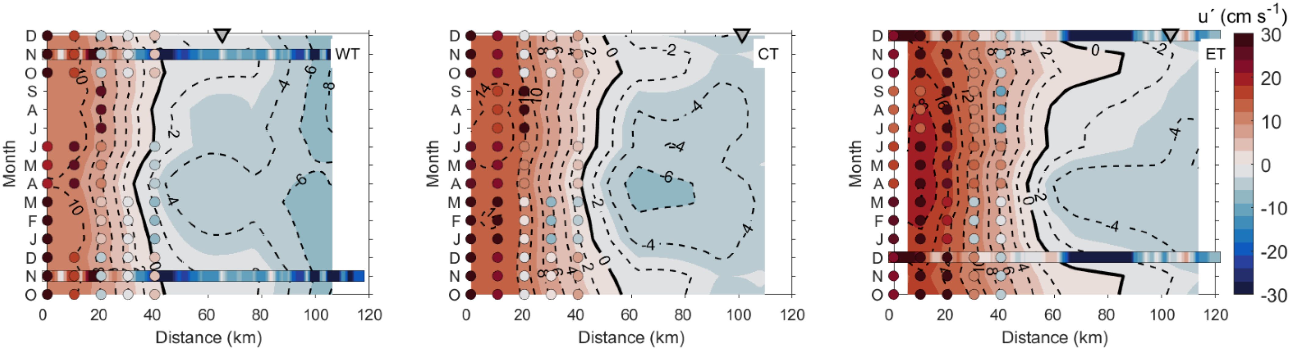
Figure 3. Hovmöller diagram of monthly climatology of altimeter-derived surface geostrophic velocity (cm s^-1) across the three transects of study (WT, CT and ET; see their locations in Figure 1) using data from DUACS multimission altimeter data processing system. The climatologies are monthly-averaged from January 1993 to December 2022. The x-axis shows the distance along the transect (in km), and the y-axis represents the months of the climatological year, starting in October and continuing through to the following December to highlight the annual pattern. The widths of the transects are 105 km, 110 km, and 115 km, respectively. Positive values (shades in red) mean northeastward flows, while negative values (shades in blue) mean southwestward flows. The contour line for 0 cm s^-1 is highlighted in solid black contour. The Bransfield Current flows year-round next to the South Shetland Islands (0 km along the transect), while the Antarctic Coastal Current flows next to the Antarctic Peninsula (120 km along the transect). Inverted grey triangles represent the position of the 200 m isobath in each transect. Colored circles above each monthly section represent seasonal mean surface velocity values derived from SADCP climatologies by Veny et al. (2022). Seasonal climatological values are placed above the months they precede: summer (Jan–Mar), autumn (Apr–Jun), winter (Jul–Sep), and spring (Oct–Dec). The colored squares above each monthly section represent synoptic measurements collected along transects presented in Frey et al. (2023), after applying the same rotation to the reference system as used in our analysis. These transects were surveyed on 24 November 2017, from the Antarctic Peninsula to Livingston Island (AI54tr3_2), and on 18–19 December 2017, from Antarctic Sound to the King George Island (ASV45tr5_3; see Figure 1).

Across all three transects, the geostrophic velocities show persistent northeastward flow near the SSI and southwestward flow near the AP throughout the climatological year. This pattern reflects the presence of the BC and CC, which are relatively stable and persist year-round. For the BC, these findings align with climatological fields derived from direct velocity measurements reported by Veny et al. (2022). Regarding the CC, the continuous presence of this current along the AP throughout the year is reported here for the first time.

From west to east (Figure 3), the BC experiences a widening whereas the CC experiences a narrowing. This downstream pattern of the BC is similar to that reported by previous works (Veny et al., 2022; Frey et al., 2023). In terms of spatiotemporal variability, the spatial extent of the BC and the CC remains nearly invariant along the WT, increases toward the CT, and reaches its maximum variability in the ET, where strong seasonal variability is observed. In this context, the BC and CC exhibit widths of approximately 40 km and ca. 65 km, respectively, along the WT. Along the CT, the BC varies in width from 45 km during late summer and early autumn to 55 km in early spring whereas the CC varies from 65 km during late summer and early autumn to 55 km in early spring. Lastly, along the ET, the BC and CC exhibit prominent across-strait excursions. The BC reaches its maximum extension of 85 km in spring, while the CC contracts to a minimum of 30 km. Conversely, from summer to early autumn, the BC reduces its extent to 55 km, whereas the CC expands to a maximum of 60 km.

In terms of current speed, the BC also experiences a strengthening up to King George Island, with maximum velocities of 10 cm s^-1 throughout all the year when closest to the Bellingshausen Sea (WT), and maximum velocities of 18 cm s^-1 from mid-summer to mid-winter when closest to the Weddell Sea (ET). From east to west (downstream of the CC in Figure 3), the flow experiences a slight increase in maximum velocities from 4 cm s^-1 in late spring to mid-winter to 8 cm s^-1 in mid-winter to early spring. The CC weakens slightly toward the other seasons while maintaining a consistent southward flow.

Lastly, we compare the altimeter-derived surface geostrophic velocity with surface SADCP measurements, incorporating both seasonal climatologies (represented by circles) from Veny et al. (2022) and synoptic transects (represented by squares) from Frey et al. (2023). While the comparison reveals qualitative consistency, the SADCP velocities are quantitatively higher than the altimetry-derived fields as previously accounted for. Nevertheless, the altimetry successfully captures the BC widening and strengthening from the WT to the ET, aligning with SADCP observations. This consistency indicates that the climatological dataset is robust, benefiting from the averaging of 30 years of monthly data. Additionally, tidal error effects in the BS evident in the altimetry data become negligible through this long-term averaging (Frey et al., 2023). These findings highlight the importance of long-term satellite monitoring for analyzing spatio-temporal interactions among boundary currents in the BS, providing the baseline knowledge to assess the role of ocean-atmosphere players driving the long-term variability of the ocean circulation in the BS.

3.2 Ocean-atmosphere-ice interactions within the boundary current domain

This section examines the interaction between ocean and atmosphere through the variability of SST, air temperature and sea ice cover across the three transects. This integrated analysis aims to elucidate the ocean-atmosphere drivers that influence the interplay of forcing mechanisms governing the boundary currents.

Figure 4 presents the monthly climatology of SST across the three transects. Highest temperatures (in red shades) appear from January to March (summertime) while lowest temperatures (in blue shades) prevail from June to November (winter to early spring) across all transects. The overall pattern indicates a slightly greater seasonal amplitude of SST within the BC domain (ranging from 1.4°C to -1.4°C) compared to the CC domain (ranging from 0.6°C to -1.7°C).

Figure 4

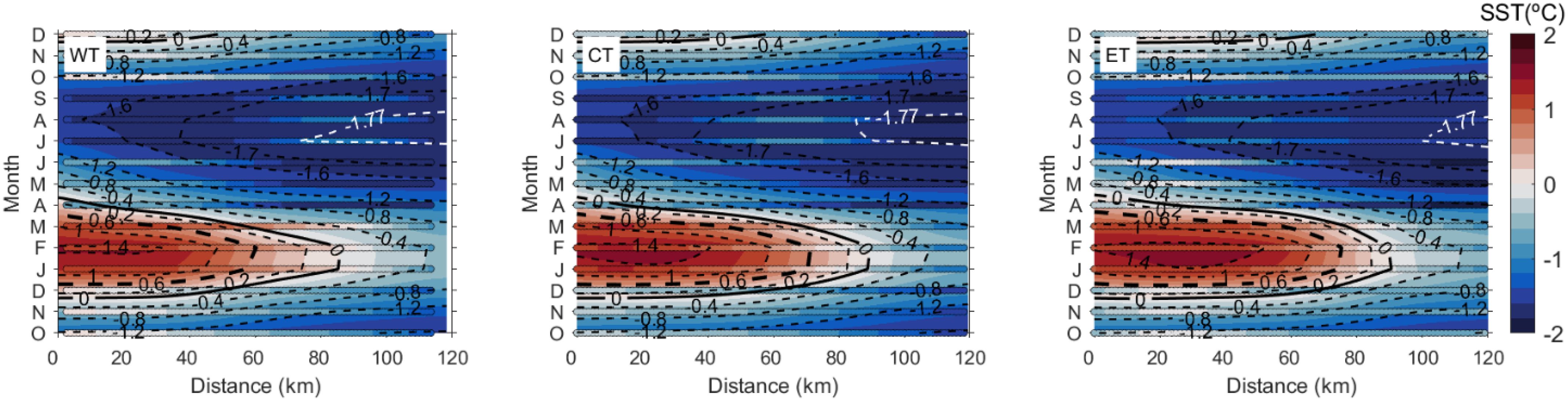
Figure 4. Hovmöller diagram of monthly climatology of Sea Surface Temperature (SST; °C) across the three transects of study (WT, CT and ET; see their locations in Figure 1) using data from OSTIA. The climatologies are monthly-averaged from January 1993 to December 2022. Positive SSTs are shown in red, while negative SSTs are shown in blue. The thick dashed black contour indicates the position of the isotherm of 0.6°C (proxy of the Peninsula Front as suggested in Veny et al., 2024). The isotherm of 0°C is highlighted in thick solid black contour. The isotherm of -1.77°C is indicated in white as a reference contour for near-freezing waters [closest to the freezing-point temperature of -1.88°C for waters with a salinity of 34.35, the threshold between TBW and TWW (Sangrà et al., 2017)], where sea ice coverage is expected. Horizontal colored lines above each monthly section represent seasonal mean surface temperature values derived from Dotto et al. (2021) seasonal climatologies. Seasonal climatological values are placed above the months they precede: summer (Jan–Mar), autumn (Apr–Jun), winter (Jul–Sep), and spring (Oct–Dec).

The warming period exhibits the same duration across the transects but features a broader and warmer pool of water downstream of the BC, particularly in the central and eastern transects. This occurs in accordance with the downstream widening of the BC (Figures 3, 4). During this period, the isotherm of 0.6°C works out as a proxy of the PF as indicated in Veny et al. (2024). The PF appears more prominently from mid-December to mid-March, extending up to 60 km from the SSI along the WT, and up to 70-80 km along the CT and ET. Here, the ET shows the most extensive warming, with temperatures reaching 1.4°C within 0 to 50 km from the SSI, while in the WT and CT, this area extends toward 30–40 km from the SSI.

The cooling period also exhibits the same duration across the transects, from April to September (autumn to winter). However, the extent of the minimum temperature coverage is greater in the WT, as indicated by the -1.6°C and -1.7°C isotherms approaching the SSI. During the sea ice season, the -1.7°C isotherm [close to the freezing-point temperature of -1.88°C for waters with a salinity of 34.35, the threshold between TBW and TWW (Sangrà et al., 2017)], covers distances from 40 to 120 km near the AP; encompassing the domain of the CC.

To further frame our findings, the monthly SST climatologies are compared with seasonal climatologies of in situ temperatures (represented by horizontal colored lines in Figure 4) from Dotto et al. (2021). It is important to highlight that the seasonal dataset is compared against monthly values in this analysis, requiring the repetition of seasonal values across three consecutive months. This comparison highlights potential differences arising from the distinct temporal resolutions of the datasets. The results reveal a spatial coherence, with each dataset exhibiting strong qualitative and quantitative similarity.

The spatial and temporal variability of the air temperature fields in BS is presented in Figure 5. The atmosphere warming period exhibits an analogous pattern as observed in the ocean: the duration across the transects is the same, featuring a broader extent and warmer air temperatures downstream of the BC, particularly in the CT and ET (the 0°C isotherm extends up to 110–120 km in the CT and ET, compared to 100 km in the WT). Conversely, air temperatures decrease over the CC domain more sharply and persist for a longer cooling period near the Bellingshausen Sea, reaching values as low as -10°C, compared to the Weddell Sea, where minimum air temperatures are around -8°C.

Figure 5

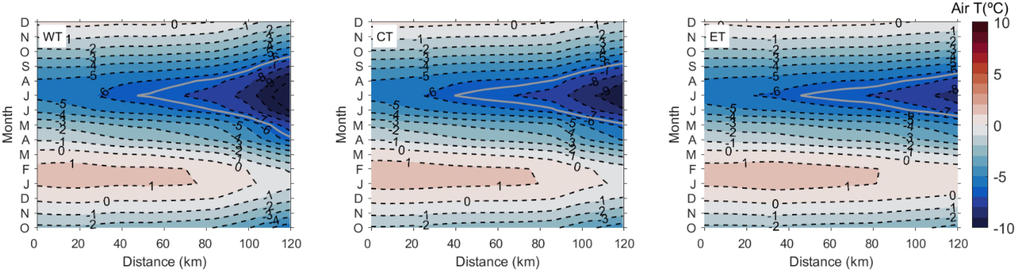
Figure 5. Hovmöller diagram of monthly climatology of air temperature (°C) across the three transects of study (WT, CT and ET; see their locations in Figure 1) using data from ERA5. The climatologies are monthly-averaged from January 1993 to December 2022. Positive temperatures are shown in red, while negative temperatures are shown in blue. The isotherm of -6.5°C is highlighted in thick solid gray contour.

By comparing Figures 4 and 5, the coupling between SST and air temperature becomes evident. Air temperature values (Figure 5) are generally higher along the SSI than near the AP, closely mirroring the spatial distribution of SST patterns (Figure 4). Notably, the -1.7°C SST isotherm, which is close to near-freezing waters (-1.77°C in Figure 4) and potential sea ice presence, consistently corresponds to air temperatures of approximately -6.5°C.

During summertime, SST peaks (Figure 4) over the BC show a 15-day lag relative to periods of highest air temperature (Figure 5). Specifically, atmospheric temperatures peak at approximately 1°C in mid-January, whereas ocean temperatures reach their maximum of 1.4°C in early February. During winter, the coldest temperature conditions over the CC are reached in July, with air temperatures ranging from -10°C in the WT to -8°C in the ET, while ocean temperatures remain above -1.7°C. Notably, one month later, the ocean extends the area embedded by the -1.6°C isotherm, reflecting a delayed oceanic response to atmospheric cooling.

The spatial and temporal variability of SIC across the transects is presented in Figure 6. A SIC percentage of 15% is the threshold for considering significant sea ice presence, which starts in May through all the three transects and remains until October (Figure 6). The timing and extent of SIC show a strong relationship with air temperature fields (Figure 5), particularly over the CC domain during late autumn through early spring. Sea ice begins forming in May across all transects when air temperatures drop below 0°C, and its presence persists until October. This coincides with the cooling phase of the air temperature fields.

Figure 6

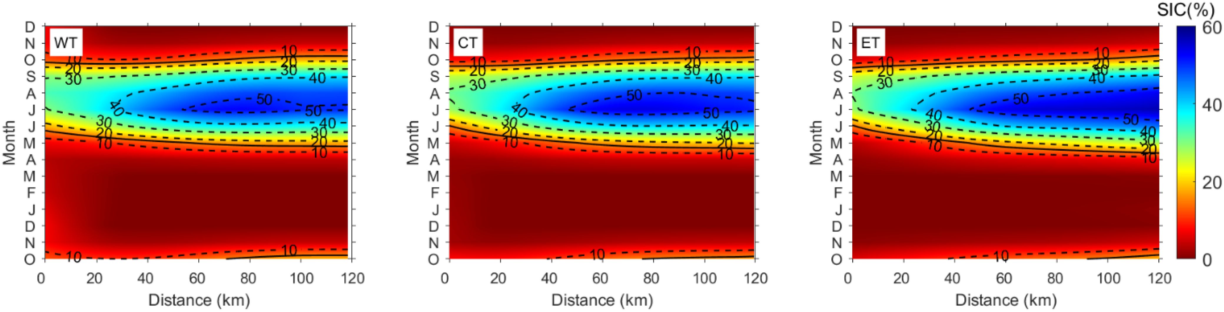
Figure 6. Hovmöller diagram of monthly climatology of Sea Ice Coverage (SIC; %) across the three transects of study (WT, CT and ET; see their locations in Figure 1) using data from OSTIA. The climatologies are monthly-averaged from January 1993 to December 2022. Regions with the lowest SIC are represented in red, while those with the highest SIC are depicted in blue. The solid black line represents the 15% SIC threshold, indicating the minimum value for significant sea ice presence.

Notably, SIC reaches maximum values of 50% in July, aligning with the coldest ocean and air temperatures (Figures 4, 5). However, the area with SIC exceeding 50% is larger along the AP and near the Weddell Sea (ET), where air temperatures are slightly higher than those near the Bellingshausen Sea (WT; Figure 5). This seemingly counterintuitive pattern reflects the influence of oceanic forcing on sea ice formation, as waters near the Weddell Sea are colder than those near the Bellingshausen Sea (Figure 4), promoting more extensive sea ice development despite the relatively higher atmospheric temperatures.

The lagged oceanic response, as described previously, and evident in the expansion of the -1.6°C SST isotherm one month after the coldest air temperatures are recorded, is also reflected in the broader extent of sea ice coverage in the WT. Here, SIC exceeds 30%, spreading extensively over the larger area covered by the -1.6°C isotherm near the SSI, highlighting the close interplay between oceanic cooling and sea ice formation dynamics. The SIC retreats completely during spring across all transects, mirroring the warming period observed in both air and ocean temperature fields. This pattern underscores the combined influence of atmospheric and oceanic forcing in governing sea ice dynamics within the region (Vorrath et al., 2020).

3.3 Wind stress forcing and surface geostrophic velocities: correlation analysis

This section aims to examine the relationship between wind stress forcing and surface geostrophic velocities in the BC and CC, focusing on seasonal and spatial variations across the three transects of study. The Hovmöller diagram of monthly climatology of wind stress (Figure 7) rotated 36.25° counterclockwise to align with the strait axis provides a detailed representation of the wind stress forcing on the BC and the CC across the three transects of study. This orientation highlights the along-strait wind stress variability, revealing seasonal patterns that drive significant changes in the dynamics and spatial extent of the BC and CC.

Figure 7

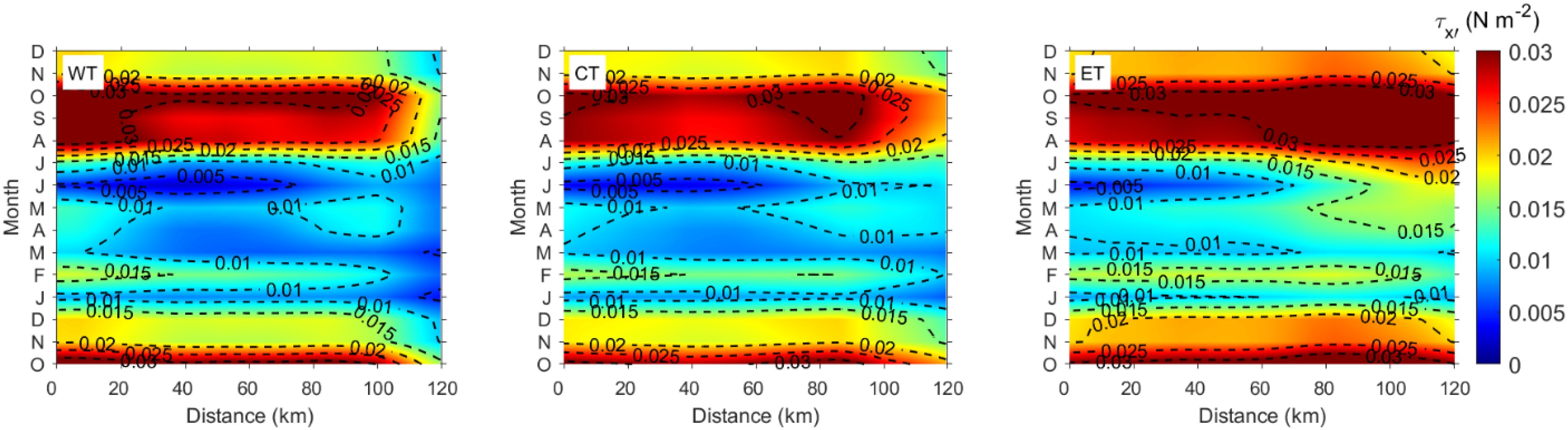
Figure 7. Hovmöller diagram showing the monthly climatology of wind stress (N m^-2) rotated 36.25° counterclockwise to align with the strait axis, illustrating the wind stress forcing on the Bransfield Current (BC) and Antarctic Coastal Current (CC) across the three transects of study (WT, CT and ET; see their locations in Figure 1) using data from ERA5. The climatologies are monthly-averaged from January 1993 to December 2022.

Elevated wind stress values (${\tau }_{x\text{'}}$ >0.015 N m^-2; Figure 7) occur predominantly during winter and spring (July–December), peaking at ${\tau }_{x\text{'}}$≈0.03 N m^-2 in October, increasing the BC strength from the WT to the ET (Figure 3), and coinciding with low SST and air temperatures (Figures 4, 5). During this period, the BC exhibits broader spatial extents (~40 km along the WT, ~55 km along the CT, and ~80 km along the ET; Figure 3, where u’ >0 cm s^-1), while the CC narrows significantly (~65 km along the WT, ~55 km along the CT, and ~35 km along the ET; Figure 3, where u’<0 cm s^-1). This agrees with the notion that westerlies (i.e. regional wind stress forcing) favor the BC while opposing the CC (Vorrath et al., 2020; Wang et al., 2022).

To quantify this relationship, we compute the correlation between rotated velocities from altimeter-derived currents (Figure 3) and wind stress using monthly climatological data (Figure 8). The results reveal that wind stress forcing exhibits varying influence across the transects, with differences in magnitude and spatial extent.

Figure 8

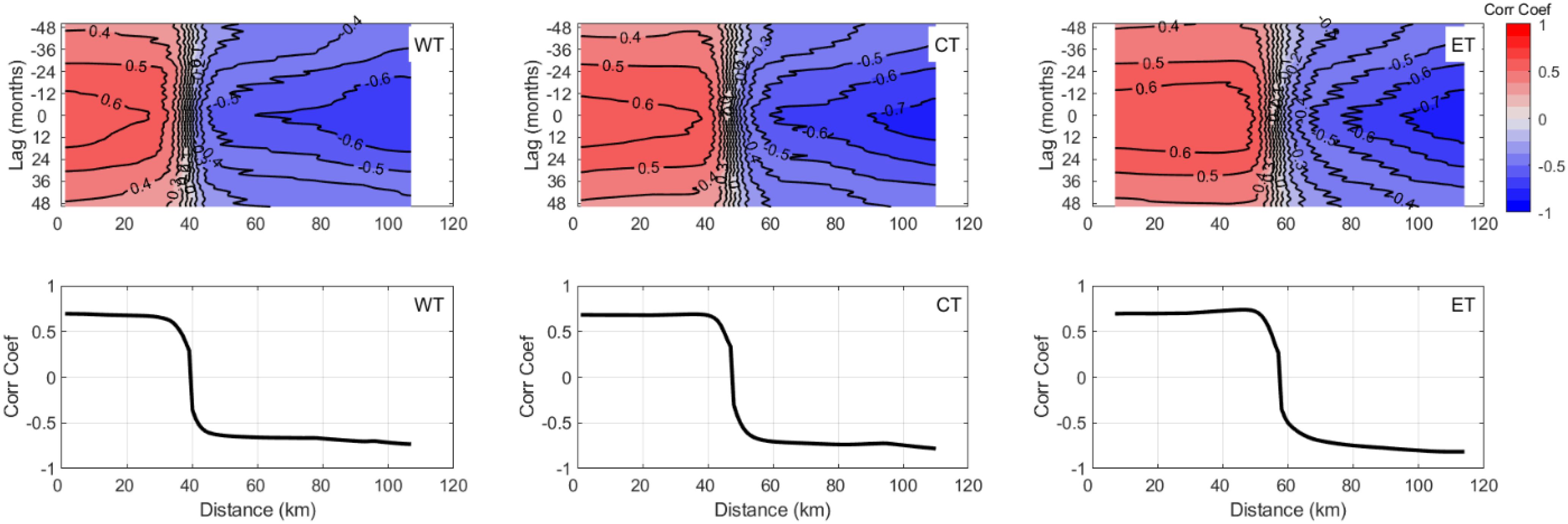
Figure 8. Correlations between monthly rotated altimeter-derived surface geostrophic velocity and wind stress across the three transects of study (WT, CT and ET; see their locations in Figure 1). Data used covers the period from January 1993 to December 2022. From top to bottom, each panel shows a Hovmöller diagram of correlation coefficients with varying monthly lag along each transect and the maximum correlation at each distance along the transect.

A significant high positive correlation, greater than 0.6 (p-value < 0.05), is observed between the BC velocity field and wind stress across much of the BS. This relationship indicates that increases in wind stress correspond to a strengthening of the northeastward-flowing BC. This behavior aligns with the previously identified widening of the BC under elevated wind stress conditions, as illustrated in Figures 3 and 7. The positive correlation extends over a broader domain upstream of the CC, reflecting the BC widening, particularly in the ET transect (Figure 8). The correlation coefficient gradually diminishes to zero at increasing distances from the SSI, marking the transition zone between the BC and CC along the three transects of study, consistent with Figure 3.

Beyond this transition zone, the correlation turns negative, ranging between -0.7 and -0.6 (p-value < 0.05), indicating that as wind stress increases, the southwestward-flowing CC tends to weaken. This inverse relationship is strongest upstream of the CC (ET in Figure 8), with negative correlation values greater than -0.7 (p-value < 0.05). This pattern reflects the opposing directions of wind stress and CC flow, where increased wind stress hinders the CC strength.

These results align with previous modelling studies (e.g., Vorrath et al., 2020; Wang et al., 2022), and assess quantitatively for the first time the influence of wind-driven dynamics on the western boundary currents in the BS based on climatological satellite observations. An open question relates to the climatological forcings at deeper layers, which are governed by other mechanisms such as baroclinic instabilities or density gradients (Sangrà et al., 2011, 2017).

3.4 Monthly climatology of near-surface volume and heat transport and interbasin balances

The near-surface interbasin volume and heat exchange is analyzed through the monthly climatological volume and heat transports, along with the associated balances across the three transects of study. The estimates, represented by red lines for the BC and blue lines for the CC, illustrate the variability over the year. The volume transport was derived from altimeter-derived geostrophic velocities (Figures 9a–d), whereas heat transport was computed using surface geostrophic velocities combined with seasonal climatological temperature profiles (Figures 9e–h) from Dotto et al. (2021), and satellite-derived sea surface temperatures (Figures 9i–l), as described in Section 2.4. The volume transport estimates of the CC were converted to positive to avoid overly broad axis limits in the graphical representation. However, we must note that these values are inherently negative, as they correspond to the southwestward flow of the CC. Lastly, the transport estimates are constrained to the surface layer, down to a depth of 100 meters. This approach adopts a conservative assumption to ensure the robustness of the results, as the analysis focuses on the upper 100 meters, where wind stress forcing and sea-ice formation processes play a major role in ocean dynamics. In contrast, SST calculations are confined to the uppermost 10 meters. Regarding the heat transport estimates, we note that both boundary currents transport water masses above the freezing point, which is used here as the reference temperature (see Section 2.4). Thus, in Figure 9, positive heat transport values for the BC (red lines) indicate northeastward transport of relatively warm waters originating from the Bellingshausen Sea and Gerlache Strait, while positive heat transport values for the CC (blue lines) indicate southwestward transport of relatively cold waters originating from the Weddell Sea.

Figure 9

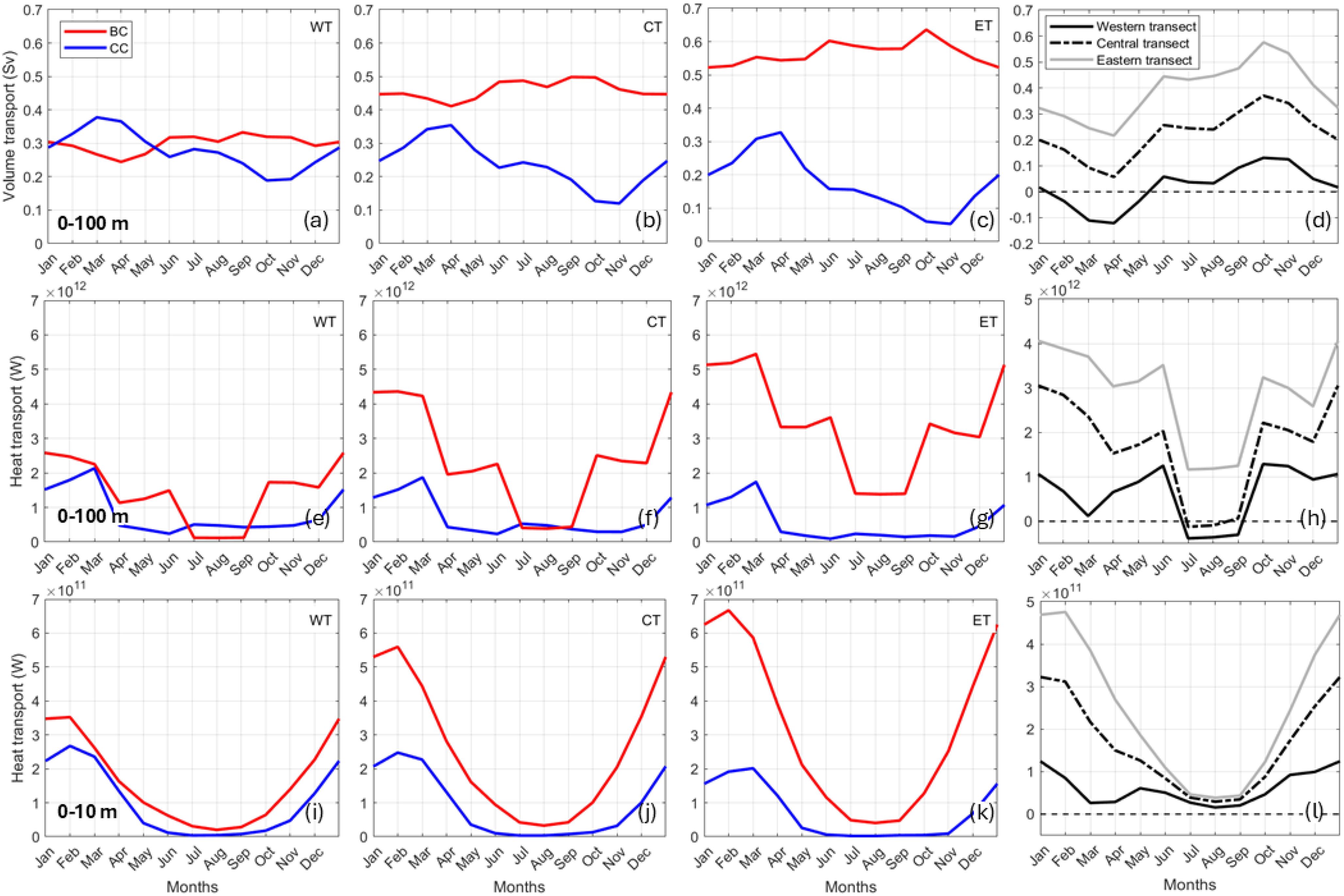
Figure 9. Monthly climatology of near-surface (a–d) volume (0-100 m), and (e–h, i–l) heat transport using Dotto et al. (2021) seasonal climatologies (0-100 m) and Sea Surface Temperature (0-10 m), respectively, across the three transects of study (WT, CT and ET; see their locations in Figure 1). The climatologies are monthly-averaged from January 1993 to December 2022. Seasonal climatological values from Dotto et al. (2021) are placed above the months they precede: summer (Jan–Mar), autumn (Apr–Jun), winter (Jul–Sep), and spring (Oct–Dec). Bransfield Current (BC) volume transport to the northeastward is shown in red, while Antarctic Coastal Current (CC) volume transport to the southwestward is shown in blue. The right-hand panels are the respective balances between the BC and the CC.

3.4.1 Volume transport

Across all three transects (Figures 9a–c), the volume transport calculated down to 100 m shows that the CC exhibits a consistent annual cycle and greater variability compared to the BC. The highest seasonal amplitude is observed in the ET, with an overall decline in volume transport as it progresses eastward (downstream of the CC). The seasonal amplitude oscillates between minimum values in spring and maximum values in summer, as follows: 0.05–0.33 Sv in the ET; 0.12–0.35 Sv in the CT; and, 0.19–0.38 Sv in the WT. Differently, the BC volume transport remains relatively stable across all transects, with a seasonal amplitude of 0.1 Sv and a slight gradual transport increase from west to east transects. The seasonal amplitude of the BC volume transport oscillates between minimum values in summer and maximum values in spring, as follows: 0.24–0.33 Sv in the WT, 0.41–0.50 Sv in the CT, and 0.52–0.64 Sv in the ET.

The pattern suggests opposing dynamics between the systems, particularly across the WT and CT, which become more pronounced through mid-summer, mid-autumn, and spring. During these seasons, BC volume transport increases as CC volume transport decreases, and vice versa, highlighting their contrasting seasonal behavior.

The observed spatio-temporal variability in the volume transport of the BC and the CC provides a broader seasonal perspective compared to findings reported in the literature, and based on observations. Only two previous studies (Savidge and Amft, 2009; Veny et al., 2022) present climatological estimates for the BC volume transport derived from direct velocity measurements over extended observation periods. In both cases, the description of the CC was prevented due to a lack of observations. The first study, Savidge and Amft (2009), could only report climatological transport values for the BC during summer. Their results showed that the transport (40–375 m depth) increases, particularly doubling from approximately 1 Sv near Boyd Strait to around 2 Sv east of Livingston Island, and remaining high further east, aligning with our observations. The second study, Veny et al. (2022), reported volume transport values (30–250 m depth; their Figure 8) for the BC across all seasons. Their findings also demonstrated a consistent increase in BC volume transport, almost doubling from Livingston Island (0.71 ± 0.14 Sv) to King George Island (1.55 ± 0.22 Sv), which is consistent with the results presented in this study. Lastly, Veny et al. (2022) reported that downstream of Nelson Strait, volume transport estimates showed no significant seasonal differences, averaging 1.31 ± 0.20 Sv. Similarly, our study observes no significant differences across seasons but extends this observation to the entire shelf of the SSI.

More recently, Gordey et al. (2024) also reported reduced spatial variability in the along-strait transport of the BC and CC down to 600 m depth with average values of 1.5–1.8 Sv and 0.7–0.8 Sv, respectively. This description was achieved following direct velocity measurements collected from 108 transects conducted during eight cruises in the austral summers (November–March) between 2015 and 2022. This highlights the complementary nature of studies based on long-term synoptic transects and climatological approaches in characterizing transport dynamics across the strait.

Regarding the volume transport driven by the CC, to the best of our knowledge no previous studies in the literature have addressed its seasonal variability from an observational perspective. For a detailed review of volume transport estimates for the BC, the reader is referred to Table 1 in Veny et al. (2022).

Compared to previous studies, it must be noted that their transport values were calculated using integration depths different from those in this work, where the focus remains on the near-surface layer. However, when comparing spatial and temporal differences, the results remain consistent. Volume transport estimates align with an increase in BC transport toward King George Island (Sangrà et al., 2017; Veny et al., 2022; Frey et al., 2023), while providing a more comprehensive seasonal perspective and broader spatial coverage across the entire SSI shelf. The findings also align with Veny et al. (2022), further revealing more stable seasonal dynamics over a broader area. Additionally, the downstream increase of CC transport reported by Gordey et al. (2024) within BS (their Figure 8) is also consistent with our results, where we expand the report of this feature throughout the year noting a marked seasonal cycle (Figure 9). These results enhance the current understanding of BC and CC volume transport by providing a more detailed and seasonally resolved view of their variability.

3.4.2 Volume transport balance

When evaluating the volume transport balance to quantify the water exchange between the inflow and outflow from the Bellingshausen and Weddell seas through the BS (Figure 9d), we recover the negative sign of the CC’s volume transport to preserve the opposite direction of its flow. The following patterns are observed.

On the one hand, the volume transport balance shows a negative slope, across all transects, from spring to summer (October to March), with values transitioning from negative to positive eastward. Minimum values are observed in all cases through the summer-to-autumn transition (March and April): -0.12 Sv in the WT, 0.06 Sv in the CT, and 0.22 Sv in the ET. Through the spring-to-summer transition (December to January), the balance crosses 0 Sv in the WT and approaches 0 Sv in the CT between March and April (0.06 Sv), when the BC and CC transport similar water volumes in opposite directions. On the other hand, the volume transport balance shows a positive slope, across all transects, from autumn to winter (April to September), with higher values eastward. Maximum values are observed in all cases through the winter-to-spring transition (September to October): 0.13 Sv in the WT, 0.37 Sv in the CT, and 0.58 Sv in the ET. Through the autumn-to-winter transition (May to July), the balance crosses 0 Sv in the WT and stays near zero throughout this period. Lastly, it is important to note that the seasonal amplitude of the volume transport balance increases from west to east, as evidenced by the differences between minimum and maximum estimates: 0.25 Sv in the WT, 0.31 Sv in the CT, and 0.36 Sv in the ET.

The above results suggest that within the first 100 m, the BS experiences a greater water mass imbalance closer to the Weddell Sea, while approaching equilibrium nearer to the Bellingshausen Sea. No previous studies have addressed the volume transport balance in the BS, which prevents further discussion in comparison with the existing literature.

3.4.3 Heat transport

Following the examination of volume transport, we address the heat fluxes across the BS, which are influenced by the interactions of velocity fields and temperature distributions. Thus, heat transport also exhibits distinct patterns across currents and transects (Figures 9e–g, i–k). Unlike volume transport, the heat transport of the BC shows a larger annual cycle and greater variability than the CC, with the seasonal amplitude increasing eastward. In contrast, the CC exhibits a smaller seasonal amplitude that decreases eastward upstream.

When heat transport computed from the Dotto et al. (2021) datasets down to 100 m (Figures 9e–g) is compared to the OSTIA datasets, which are confined to the upper 10 m (Figures 9i–k), similar seasonal patterns are observed. However, the OSTIA-derived results appear smoother, likely due to the inherent characteristics of each seasonal climatology, with OSTIA benefiting from regular and more systematic measurements, adding finer resolution to the seasonal variability.

For the temperature dataset from Dotto et al. (2021) (Figures 9e–g), the seasonal amplitude of heat transport driven by the BC varies from winter minima to summer maxima, with ranges as follows (higher maxima increasing eastward, downstream the BC): 0.12x10¹² to 2.58x10¹² W in the WT; 0.39x10¹² to 4.36x10¹² W in the CT; and, 1.38x10¹² to 5.44x10¹² W in the ET. When using the OSTIA temperature dataset (Figures 9i–k), the seasonal amplitude exhibits similar variability, with ranges as follows (higher maxima also increasing eastward, downstream the BC): 0.20x10¹¹ to 3.52x10¹¹ W in the WT; 0.33x10¹¹ to 5.59x10¹¹ W in the CT; and, 0.41x10¹¹ to 6.67x10¹¹ W in the ET.

In contrast, for the temperature dataset from Dotto et al. (2021) (Figures 9e–g), the heat transport driven by the CC exhibits lower seasonal variability, oscillating between an autumn minimum and a summer maximum, with ranges as follows (maximum estimates slightly decreasing eastwestward, upstream the BC): 0.24x10¹² to 2.13x10¹² W in the WT; 0.23x10¹² to 1.87x10¹² W in the CT; and, 0.09x10¹² to 1.74x10¹² W in the ET. When using the OSTIA temperature dataset (Figures 9i–k), the seasonal variability follows a similar pattern, but in this case the minimum is in winter, with ranges as follows: 0.04x10¹¹ to 2.67x10¹¹ W in the WT; 0.03x10¹¹ to 2.48x10¹¹ W in the CT; and, 0.02x10¹¹ to 2.02x10¹¹ W in the ET.

These results highlight the marked seasonal and spatial variability of the BC, which transports water masses towards the northeast in the BS. These waters are seasonally originated in the Bellingshausen Sea and Gerlache Strait, where significant seasonal temperature fluctuations exist due to summer heating and ice melting (Tokarczyk, 1987; García et al., 1994; Sangrà et al., 2011). Meanwhile, the CC transports more homogeneous water masses toward the southwest in the BS. These waters are originated in the Weddell Sea, exhibiting lower seasonal temperature variability due to a more limited response to seasonal thermal forcing (Grelowski et al., 1986; Tokarczyk, 1987; García et al., 1994; Hofmann et al., 1996; García et al., 2002; Zhou et al., 2002).

3.4.4 Heat transport balance

When evaluating the heat transport balance to quantify the heat exchange between the inflow and outflow from the Bellingshausen and Weddell seas through the BS (Figures 9h, l), we recover the negative sign of the CC volume transport to preserve the opposite direction of the boundary currents. Thus, positive values of the heat transport balance indicate a larger heat transport driven by the BC, contributing to a surplus of heat towards the northeast. Conversely, negative values of the heat transport balance indicate a larger heat transport driven by the CC, contributing to a surplus of heat towards the southwest.

Overall, heat transport balances computed from the temperature climatology developed in Dotto et al. (2021) and the OSTIA dataset (Figures 9h and l, respectively) indicate a reduction in net heat transport during winter, particularly between July and August. This reduction may be attributed to the more homogeneous temperatures across the strait during this period and the larger sea-ice coverage, which reduces heat exchange between the ocean and the atmosphere. For heat transport estimates based on Dotto et al. (2021), the net balance (0–100 m depth) during winter approaches zero in the western and central transects, increasing to higher positive values towards the eastern transect.

For heat transport estimates based on OSTIA (0–10 m depth), the general pattern is analogous, with a notable difference: the net heat transport in the three transects of study approaches zero in winter (July and August), extending for a longer period year-round in the WT but in spring and early summer. When examining whether this feature also applies to estimates based on Dotto et al. (2021) but limited to the top 10 m of the water column, we observe a similar pattern. This suggests that the mismatch in net heat transport estimates in Figures 9h, l can be attributed to the different vertical extent considered in the computations.

Through spring, both net heat transports (Figures 9h, l) increase, reaching their maximum values in January before beginning a decreasing trend. This pattern becomes more pronounced moving eastward. This indicates that heat exchange is more prominent near the Weddell Sea and less prominent near the Bellingshausen Sea during spring and summer. These results provide the first comprehensive overview of the heat transport balance driven by the boundary currents of the BS.

4 Conclusions

This study provides a comprehensive analysis of the near-surface layers of the boundary currents in the BS, using 30 years of multi-platform satellite data to assess their spatiotemporal variability and contributions to interbasin exchange.

The BC exhibits consistent strengthening up to King George Island across all seasons, with altimeter-derived volume transport (0–100 m depth) increasing from 0.24–0.33 Sv in the western transect to 0.52–0.64 Sv in the eastern transect in the BS, while decreasing downstream as it recirculates around the SSI. Heat transport peaks in summer, reaching 5.44x10¹² W based on hydrographic climatology estimates (0–100 m depth; Dotto et al., 2021) and 6.67x10¹¹ W derived from the OSTIA SST product (0–10 m depth). In contrast, the CC displays pronounced seasonality in volume transport (0-100 m depth), oscillating between 0.19–0.38 Sv in the western transect and 0.05–0.33 Sv in the eastern transect in the BS. Its heat transport also peaks in summer, reaching 2.13x10¹² W (0–100 m depth; Dotto et al., 2021) and 2.67x10¹¹ W (OSTIA; 0–10 m depth), respectively.

A key finding is the heat transport balance approaching zero during winter, particularly in the western transect, driven by homogeneous temperatures (due to wind-driven mixing) and extensive sea ice coverage. This marks periods of reduced interbasin heat exchange and highlights the interplay between temperature gradients, wind stress, and sea ice extent in regulating the boundary currents and local hydrography. Notably, significant positive correlations are observed between the BC and along-strait wind stress, suggesting its near-surface variability is strongly influenced by wind forcing. The CC, in comparison, displays weaker but consistent negative correlations with along-strait wind stress, indicating a distinct response to atmospheric forcing compared to the BC. These findings highlight the asymmetric contributions and forcings of the BC and CC in shaping regional hydrography, sea ice dynamics, and interbasin exchange. Furthermore, the position and strength of the PF are found to be closely tied to the distinct volume and heat transport driven by these currents, with potential impacts on local ecosystem structure and function (Veny et al., 2024).

The Appendix presents critical findings from the analysis of surface drifter data and two open-access global ocean reanalysis products, offering complementary insights into the boundary currents of the BS. On the one hand, surface drifter data confirm the downstream broadening of the BC as a coherent northeastward-flowing jet and the continuous nature of the CC flowing southwestward along the AP during summertime, emphasizing the challenges of fully characterizing their year-round variability from direct velocity measurements. On the other hand, the open-access global ocean reanalysis products (GLORYS12V1 and HYCOM) are found to inadequately represent the BS circulation. Neither product captures the CC as a continuous and spatially coherent feature, nor do they reproduce the observed heat transport balances (not shown). These limitations emphasize the importance of integrating high-resolution observational data and advancing model capabilities to better resolve boundary current dynamics in this region.

Overall, this study establishes a critical baseline for understanding climate-driven changes in the near-surface layers of the boundary currents of the BS, including shifts in volume and heat budgets, with implications for glacier melt, sea ice persistence, and, ultimately, broader Southern Ocean circulation. Future research should focus on subsurface dynamics to complement these insights, as well as on the impacts of long-term climate variability on the coupled ocean-atmosphere-ice system in the AP region.

Data availability statement

The original contributions presented in the study are included in the article and Supplementary Material. Further inquiries can be directed to the corresponding authors.

Author contributions

MV: Writing – original draft, Conceptualization, Data curation, Formal analysis, Investigation, Methodology, Software, Validation, Visualization. BA-G: Writing – original draft, Conceptualization, Data curation, Formal analysis, Funding acquisition, Investigation, Methodology, Software, Supervision, Validation, Visualization. AR-U: Writing – review & editing, Data curation, Software, Visualization. TP-V: Writing – review & editing, Data curation, Software, Visualization. LP-A: Writing – review & editing, Software, Visualization. ÁM-D: Writing – review & editing, Methodology, Supervision.

Funding

The author(s) declare that financial support was received for the research and/or publication of this article. This work has been supported by the Spanish government (Ministerio de Economía y Competitividad) through the projects e-IMPACT (PID2019-109084RB-C21) and COUPLING II (PID2023-148583NB-C21). Additional support was provided by the project PLANCLIMAC2 (1/MAC/2/2.4/0006) from the INTERREG VI Territorial Cooperation Program (MADEIRA-AZORES-CANARIAS MAC 2021-2027). The first author is also grateful to the Canary government (Agencia Canaria de Investigación, Innovación y Sociedad de la Información de la Consejería de Universidades, Ciencia e Innovación y Cultura) and to the Fondo Social Europeo Plus (FSE+) Programa Operativo Integrado de Canarias 2021-2027, Eje 3 Tema Prioritario 74 (85%), for the financial support awarded through a PhD scholarship (TESIS2021010025).

Acknowledgments

We thank the two reviewers of this study for their time and dedication in providing us with suggestions and comments that have significantly helped improve our work.

Conflict of interest

The authors declare that the research was conducted in the absence of any commercial or financial relationships that could be construed as a potential conflict of interest.

The author(s) declared that they were an editorial board member of Frontiers, at the time of submission. This had no impact on the peer review process and the final decision.

Generative AI statement

The author(s) declare that Generative AI was used in the creation of this manuscript. ChatGPT, developed by OpenAI, was used for proofreading of this manuscript.

Publisher’s note

All claims expressed in this article are solely those of the authors and do not necessarily represent those of their affiliated organizations, or those of the publisher, the editors and the reviewers. Any product that may be evaluated in this article, or claim that may be made by its manufacturer, is not guaranteed or endorsed by the publisher.

Supplementary material

The Supplementary Material for this article can be found online at: https://www.frontiersin.org/articles/10.3389/fmars.2025.1555552/full#supplementary-material

References

Annasawmy P., Horne J. K., Reiss C. S., Cutter G. R., Macaulay G. J. (2023). Antarctic krill (Euphausia superba) distributions, aggregation structures, and predator interactions in Bransfield Strait. Polar Biol. 46, 151–168. doi: 10.1007/s00300-023-03113-z

Crossref Full Text | Google Scholar

Atkinson A., Siegel V., Pakhomov E., Rothery P. (2004). Long-term decline in krill stock and increase in salps within the Southern Ocean. Nature 432, 100–103. doi: 10.1038/nature02996

PubMed Abstract | Crossref Full Text | Google Scholar

Barré N., Provost C., Renault A., Sennéchael N. (2011). Fronts, meanders and eddies in Drake Passage during the ANT-XXIII/3 cruise in January–February 2006: A satellite perspective. Deep Sea Res. Part II: Top. Stud. Oceanogr. 58, 2533–2554. doi: 10.1016/j.dsr2.2011.01.003

Crossref Full Text | Google Scholar

Cook A. J., Holland P. R., Meredith M. P., Murray T., Luckman A., Vaughan D. G. (2016). Ocean forcing of glacier retreat in the western Antarctic Peninsula. Science 353, 283–286. doi: 10.1126/science.aae0017

PubMed Abstract | Crossref Full Text | Google Scholar

Dotto T. S., Mata M. M., Kerr R., Garcia C. A. (2021). A novel hydrographic gridded data set for the northern Antarctic Peninsula. Earth Sys. Sci. Data 13, 671–696. doi: 10.5194/essd-13-671-2021

Crossref Full Text | Google Scholar

Ducklow H. W., Fraser W. R., Meredith M. P., Stammerjohn S. E., Doney S. C., Martinson D. G., et al. (2013). West Antarctic Peninsula: an ice-dependent coastal marine ecosystem in transition. Oceanography 26, 190–203. doi: 10.5670/oceanog.2013.62

Crossref Full Text | Google Scholar

Eayrs C., Holland D., Francis D., Wagner T., Kumar R., Li X. (2019). Understanding the seasonal cycle of Antarctic sea ice extent in the context of longer-term variability. Rev. Geophys. 57, 1037–1064. doi: 10.1029/2018RG000631

Crossref Full Text | Google Scholar

Ferrari R., Artana C., Saraceno M., Piola A. R., Provost C. (2017). Satellite altimetry and current-meter velocities in the Malvinas Current at 41 S: Comparisons and modes of variations. J. Geophys. Res.: Oceans 122, 9572–9590. doi: 10.1002/2017JC013340

Crossref Full Text | Google Scholar

Firing E., Hummon J. M., Chereskin T. K. (2012). Improving the quality and accessibility of current profile measurements in the southern ocean. Oceanography 25, 164–165. doi: 10.5670/oceanog.2012.91

Crossref Full Text | Google Scholar

Frey D., Gladyshev S., Krechik V., Morozov E. (2021a). SADCP measurements in the Bransfield strait in 2017. Mendeley Data. doi: 10.17632/g58z4mczs7.1

Crossref Full Text | Google Scholar

Frey D., Krechik V., Gordey A., Gladyshev S., Churin D., Drozd I., et al. (2023). Austral summer circulation in the Bransfield Strait based on SADCP measurements and satellite altimetry. Front. Mar. Sci. 10, 1111541. doi: 10.3389/fmars.2023.1111541

Crossref Full Text | Google Scholar

Frey D. I., Piola A. R., Krechik V. A., Fofanov D. V., Morozov E. G., Silvestrova K. P., et al. (2021b). Direct measurements of the Malvinas Current velocity structure. J. Geophys. Res.: Oceans 126, e2020JC016727. doi: 10.1029/2020JC016727

Crossref Full Text | Google Scholar

García M. A., Castro C. G., Ríos A. F., Doval M. D., Rosón G., Gomis D., et al. (2002). Water masses and distribution of physico-chemical properties in the Western Bransfield Strait and Gerlache Strait during Austral summer 1995/96. Deep Sea Res. Part II: Top. Stud. Oceanogr. 49, 585–602. doi: 10.1016/S0967-0645(01)00113-8

Crossref Full Text | Google Scholar

García M. A., López O., Sospedra J., Espino M., Gràcia V., Morrison G., et al. (1994). “Mesoscale variability in the Bransfield Strait region (Antarctica) during Austral summer,” in Annales Geophysicae, vol. 12. (Berlin, Germany: Springer-Verlag), 856–867.

Google Scholar

García-Muñoz C., Lubián L. M., García C. M., Marrero-Díaz Á., Sangra P., Vernet M. (2013). A mesoscale study of phytoplankton assemblages around the South Shetland Islands (Antarctica). Polar Biol. 36, 1107–1123. doi: 10.1007/s00300-013-1333-5

Crossref Full Text | Google Scholar

Good S., Fiedler E., Mao C., Martin M. J., Maycock A., Reid R., et al. (2020). The current configuration of the OSTIA system for operational production of foundation sea surface temperature and ice concentration analyses. Remote Sens. 12, 720. doi: 10.3390/rs12040720

Crossref Full Text | Google Scholar

Gordey A. S., Frey D. I., Drozd I. D., Krechik V. A., Smirnova D. A., Gladyshev S. V., et al. (2024). Spatial variability of water mass transports in the Bransfield Strait based on direct current measurements. Deep Sea Res. Part I: Oceanogr. Res. Pap. 207, 104284. doi: 10.1016/j.dsr.2024.104284

Crossref Full Text | Google Scholar

Gordon A. L., Nowlin W. D. Jr. (1978). The basin waters of the Bransfield Strait. J. Phys. Oceanogr. 8, 258–264. doi: 10.1175/1520-0485(1978)008<0258:TBWOTB>2.0.CO;2

Crossref Full Text | Google Scholar

Grelowski A., Majewicz A., Pastuszak M. (1986). Mesoscale hydrodynamic processes in the region of Bransfield Strait and the southern part of Drake Passage during BIOMASS-SIBEX 1983/84. Polish Polar Res. 7, 353–369.

Google Scholar

Hersbach H., Bell B., Berrisford P., Hirahara S., Horányi A., Muñoz-Sabater J., et al. (2020). The ERA5 global reanalysis. Q. J. R. Meteorol. Soc. 146, 1999–2049. doi: 10.1002/qj.v146.730

Crossref Full Text | Google Scholar

Hofmann E. E., Klinck J. M., Lascara C. M., Smith D. A. (1996). “Water mass distribution and circulation west of the Antarctic Peninsula and including Bransfield Strait,” in Foundations for ecological research west of the Antarctic Peninsula, Washington, D.C., USA: American Geophysical Union (AGU) vol. 70, 61–80.

Google Scholar

Johnston N. M., Murphy E. J., Atkinson A., Constable A. J., Cotté C., Cox M., et al. (2022). Status, change, and futures of zooplankton in the Southern Ocean. Front. Ecol. Evol. 9, 624692. doi: 10.3389/fevo.2021.624692

Crossref Full Text | Google Scholar

King M. A., Padman L. (2005). Accuracy assessment of ocean tide models around Antarctica. Geophys. Res. Lett. 32, L23608. doi: 10.1029/2005GL023901

Crossref Full Text | Google Scholar

Lago L. S., Saraceno M., Piola A. R., Ruiz-Etcheverry L. A. (2021). Volume transport variability on the northern argentine continental shelf from in situ and satellite altimetry data. J. Geophys. Res.: Oceans 126, e2020JC016813. doi: 10.1029/2020JC016813

Crossref Full Text | Google Scholar

Lenn Y. D., Chereskin T. K., Sprintall J., Firing E. (2007). Mean jets, mesoscale variability and eddy momentum fluxes in the surface layer of the Antarctic Circumpolar Current in Drake Passage. J. Mar. Res. 65, 27–58. doi: 10.1357/002224007780388694

Crossref Full Text | Google Scholar

Loeb V. J., Hofmann E. E., Klinck J. M., Holm-Hansen O., White W. B. (2009). ENSO and variability of the Antarctic Peninsula pelagic marine ecosystem. Antarctic Sci. 21, 135–148. doi: 10.1017/S0954102008001636

Crossref Full Text | Google Scholar

Loeb V., Siegel V., Holm-Hansen O., Hewitt R., Fraser W., Trivelpiece W., et al. (1997). Effects of sea-ice extent and krill or salp dominance on the Antarctic food web. Nature 387, 897–900. doi: 10.1038/43174

Crossref Full Text | Google Scholar

López O., García M. A., Gomis D., Rojas P., Sospedra J., Sánchez-Arcilla A. (1999). Hydrographic and hydrodynamic characteristics of the eastern basin of the Bransfield Strait (Antarctica). Deep Sea Res. Part I: Oceanogr. Res. Pap. 46, 1755–1778. doi: 10.1016/S0967-0637(99)00017-5

Crossref Full Text | Google Scholar

Lumpkin R., Centurioni L. (2010). NOAA Global Drifter Program quality-controlled 6-hour interpolated data from ocean surface drifting buoys (Asheville, North California, USA: NOAA National Centers for Environmental Information). doi: 10.25921/7ntx-z961

Crossref Full Text | Google Scholar

Lüpkes C., Birnbaum G. (2005). Surface drag in the Arctic marginal sea-ice zone: A comparison of different parameterisation concepts. Boundary-Layer Meteorol. 117, 179–211. doi: 10.1007/s10546-005-1445-8

Crossref Full Text | Google Scholar

Montes-Hugo M., Doney S. C., Ducklow H. W., Fraser W., Martinson D., Stammerjohn S. E., et al. (2009). Recent changes in phytoplankton communities associated with rapid regional climate change along the western Antarctic Peninsula. Science 323, 1470–1473. doi: 10.1126/science.1164533

PubMed Abstract | Crossref Full Text | Google Scholar

Morozov E. G. (2007). Currents in bransfield strait. In doklady earth sciences (Springer Nature BV) 415, 984. doi: 10.1134/S1028334X07060347

Crossref Full Text | Google Scholar

Murzina S. A., Voronin V. P., Bitiutskii D. G., Mishin A. V., Khurtina S. N., Frey D. I., et al. (2023). Comparative analysis of the fatty acid profiles of Antarctic krill (Euphausia superba dana 1850) in the Atlantic sector of the southern ocean: certain fatty acids reflect the oceanographic and trophic conditions of the habitat. J. Mar. Sci. Eng. 11, 1912. doi: 10.3390/jmse11101912

Crossref Full Text | Google Scholar

Padman L., Fricker H. A., Coleman R., Howard S., Erofeeva L. (2002). A new tide model for the Antarctic ice shelves and seas. Ann. Glaciol. 34, 247–254. doi: 10.3189/172756402781817752

Crossref Full Text | Google Scholar

Poulin F. J., Stegner A., Hernández-Arencibia M., Marrero-Díaz A., Sangrà P. (2014). Steep shelf stabilization of the coastal Bransfield Current: Linear stability analysis. J. Phys. oceanogr. 44, 714–732. doi: 10.1175/JPO-D-13-0158.1

Crossref Full Text | Google Scholar

Sangrà P., Gordo C., Hernandez-Arencibia M., Marrero-Díaz A., Rodríguez-Santana A., Stegner A., et al. (2011). The Bransfield current system. Deep Sea Res. Part I: Oceanogr. Res. Pap. 58, 390–402. doi: 10.1016/j.dsr.2011.01.011

Crossref Full Text | Google Scholar

Sangrà P., Stegner A., Hernández-Arencibia M., Marrero-Díaz Á., Salinas C., Aguiar-González B., et al. (2017). The Bransfield gravity current. Deep Sea Res. Part I: Oceanogr. Res. Pap. 119, 1–15. doi: 10.1016/j.dsr.2016.11.003

Crossref Full Text | Google Scholar

Savidge D. K., Amft J. A. (2009). Circulation on the west antarctic peninsula derived from 6 years of shipboard ADCP transects. Deep sea research part I: oceanographic research papers 56 (10), 1633–1655. doi: 10.1016/j.dsr.2009.05.011

Crossref Full Text | Google Scholar

Schofield O., Ducklow H. W., Martinson D. G., Meredith M. P., Moline M. A., Fraser W. R. (2010). How do polar marine ecosystems respond to rapid climate change? Science 328, 1520–1523. doi: 10.1126/science.1185779

PubMed Abstract | Crossref Full Text | Google Scholar

Tokarczyk R. (1987). Classification of water masses in the Bransfield Strait and southern part of the Drake Passage using a method of statistical multidimensional analysis. Polish Polar Res. 8, 333–366.

Google Scholar

Veny M., Aguiar-González B., Marrero-Díaz Á., Pereira-Vázquez T., Rodríguez-Santana Á. (2024). Biophysical coupling of seasonal chlorophyll-a bloom variations and phytoplankton assemblages across the Peninsula Front in the Bransfield Strait. Ocean Sci. 20, 389–415. doi: 10.5194/os-20-389-2024

Crossref Full Text | Google Scholar

Veny M., Aguiar-González B., Marrero-Díaz Á., Rodríguez-Santana Á. (2022). Seasonal circulation and volume transport of the Bransfield Current. Prog. Oceanogr. 204, 102795. doi: 10.1016/j.pocean.2022.102795

Crossref Full Text | Google Scholar

Vorrath M. E., Müller J., Cárdenas P., Opel T., Mieruch S., Esper O., et al. (2023). Deglacial and Holocene sea-ice and climate dynamics in the Bransfield Strait, northern Antarctic Peninsula. Climate Past 19, 1061–1079. doi: 10.5194/cp-19-1061-2023

Crossref Full Text | Google Scholar

Vorrath M. E., Müller J., Rebolledo L., Cárdenas P., Shi X., Esper O., et al. (2020). Sea ice dynamics in the Bransfield Strait, Antarctic Peninsula, during the past 240 years: a multi-proxy intercomparison study. Climate Past 16, 2459–2483. doi: 10.5194/cp-16-2459-2020

Crossref Full Text | Google Scholar

Wang X., Moffat C., Dinniman M. S., Klinck J. M., Sutherland D. A., Aguiar-González B. (2022). Variability and dynamics of along-shore exchange on the West Antarctic Peninsula (WAP) continental shelf. J. Geophys. Res.: Oceans 127, e2021JC017645. doi: 10.1029/2021JC017645

Crossref Full Text | Google Scholar

Zhou M., Niiler P. P., Hu J. H. (2002). Surface currents in the Bransfield and Gerlache straits, Antarctica. Deep Sea Res. Part I: Oceanogr. Res. Pap. 49, 267–280. doi: 10.1016/S0967-0637(01)00062-0

Crossref Full Text | Google Scholar

Zhou X., Zhu G., Hu S. (2020). Influence of tides on mass transport in the Bransfield Strait and the adjacent areas, Antarctic. Polar Sci. 23, 100506. doi: 10.1016/j.polar.2020.100506

Crossref Full Text | Google Scholar