Real-time prediction of port water levels based on EMD-PSO-RBFNN

Addressing the spatial variability, temporal dynamics, and non-linearity characteristics of port water levels, a hybrid prediction scheme was proposed, which integrates empirical mode decomposition (EMD) with a radial basis function neural network (RBFNN), optimized using the particle swarm optimization (PSO) algorithm. First, through the application of EMD, the port water level time series was decomposed into sub-series characterized by lower non-linearity. Subsequently, PSO was applied to fine-tune the center and spread parameters of the RBFNN, thereby enhancing the model’s predictive performance. The optimized PSO-RBFNN model was employed to make predictions on the decomposed sub-series. Finally, reconstruction of the predicted sub-series yielded the final water level predictions. The feasibility and effectiveness of the proposed model were validated using measured port water level data. Results from simulations highlighted the model’s ability to deliver accurate predictions across various lead times. Furthermore, comparative analysis revealed that the proposed model outperforms alternative methods in port water level prediction. Therefore, the proposed model serves as a reliable, efficient, and real-time prediction tool, providing robust support for port operational safety.

1 Introduction

Port water level refers to the vertical distance of the water surface within a port relative to a reference plane. It is typically influenced by various factors, including waves, river flow, climatic changes, and the geological conditions of the port (Christodoulou et al., 2019; Rabinovich, 2010). The variation in port water levels is a variable process, characterized by spatial variability, temporal dynamics, and non-linear properties. Excessively high or low water levels can significantly impact port scheduling, ship entry, and departure, as well as cargo loading and unloading operations (López and Pina, 1988). In particular, during typhoons making landfall near ports, abnormally high water levels may lead to substantial economic losses. Accurate prediction of port water level is essential for port construction and design, environmental protection, vessel operations, and recreational activities. Therefore, real-time and precise predictions of port water level are critical for preventing vessel grounding, avoiding in-port collisions, managing ports and waterways, and optimizing ship scheduling.

The phenomenon of harbor resonance (López et al., 2012), caused by the interaction between harbor waters and ocean-generated waves through multiple openings, results in continuous fluctuations in the water level within the port. Additionally, tidal influences, driven by celestial bodies, impact the sea level every 12 hours. Some ports experience significant water level fluctuations at different times of the year along their navigational channels (Nur et al., 2020), and these variations have a profound impact on port operability (Gracia et al., 2019). Monitoring the port water level is a critical task. For example, Ulm et al. (2016) investigated the impact of Egmont Key’s loss on storm surge water levels and wind waves along the Tampa Bay coastline through sensitivity simulations. Appell et al. (1994) developed a port information system for Tampa Bay, Florida, which provides water level reports every 6 minutes. Deng et al. (2022) proposed a particle swarm optimization (PSO)-enhanced Elman neural network model for downstream water level prediction in Dongting Lake, with input features including upstream water station data such as water level, flow rate, rainfall, and temperature, as well as rainfall data from downstream stations. Gao et al. (2023) utilized the Bragg reflection phenomenon and monitored the characteristics of port wave height, wave motion, and water level based on arc-shaped periodic undulating topography, significantly reducing the energy of long-period oscillations within the port and effectively mitigating harbor resonance issues. However, sensor-based monitoring systems face challenges such as short monitoring periods and poor real-time capabilities. To address these issues, Dong et al. (2018) evaluated extreme port water levels using probabilistic models. Zheng et al. (2022) employed artificial neural network (ANN) models based on offshore parameters (wave height, period, and direction) to estimate wave height inside ports rapidly. López and Iglesias (2013) applied ANN models to estimate the infragravity wave heights inside harbors, demonstrating that a one-step model outperformed a two-step model in accuracy. Adnan et al. (2023) used Bayesian averaging methods to predict effective wave heights for short-term predictions. Yang et al. (2024) proposed a convolutional long short-term memory (ConvLSTM) model incorporating an attention mechanism for nearshore water level prediction. The model leverages multiscale information from historical water level data and enhances the importance of key features through the attention mechanism, thereby improving prediction accuracy and timeliness. Deo and Şahin (2016) utilized the extreme learning machine model, based on input parameters such as rainfall, sea surface temperature, and climate indices, to simulate streamflow water levels at three hydrological sites in eastern Queensland. The results demonstrated that the model could perform streamflow predictions quickly and efficiently. However, due to the uncertainty of port water level fluctuations, constructing a deterministic model that can be universally applicable to all climate types and diverse terrains is undoubtedly a highly challenging task (Ghorbani et al., 2018). Therefore, to predict port water levels accurately and in real-time, an adaptive non-linear model needs to be developed.

As advancements in intelligent computing and information processing technologies emerged in the mid-to-late 20th century, the potential for achieving real-time and accurate predictions of port water level heights was established (Juan et al., 2023). Within the broad spectrum of advanced computing approaches, neural networks have garnered significant attention due to their inherent non-linear characteristics and exceptional adaptability (Kumar et al., 2017). As an efficient machine learning model, radial basis function neural networks (RBFNNs) have exhibited superior performance across various domains including recognition, prediction, and signal processing. Notably, their rapid convergence and remarkable capability in addressing non-linear system prediction problems have made them a focal point of interest (Huo et al., 2023; Tao et al., 2021). Moreover, they are widely employed in prediction tasks within the fields of maritime and ocean engineering. For example, Wang et al. (2024) used gray relational analysis to filter network input features and employed Bayesian optimization of the RBFNN to predict ship metacentric height in real-time. Yin et al. (2018) applied discrete wavelet transform to break down the ship’s rolling motion into sub-series and employed the RBFNN to approximate the non-linear mapping for each component, ultimately achieving ship rolling motion prediction through data reconstruction. Yin et al. (2015) also employed harmonic analysis combined with the RBFNN to develop a hybrid prediction mechanism for accurate and real-time tidal prediction. Han (2021) employed a fractional gradient descent method, characterized by its flexible updating mechanism and efficient search capability, to adjust the RBFNN weights, facilitating the estimation of vessel traffic flow in ports. Cao and Zhu (2014) combined computational fluid dynamics technology with the RBFNN to predict the hydrodynamics of submarines, achieving notable accuracy and high efficiency. The accuracy of forecasts can be significantly compromised by suboptimal parameter and structure configurations in neural networks. To improve forecasting performance, swarm intelligence algorithms can be employed to optimize network parameters and structure effectively (Xu and Yin, 2024; Zhang et al., 2023).

As a tool for managing non-linear and non-stationary signals in data preprocessing, empirical mode decomposition (EMD) has recently gained significant attention (Song et al., 2023). Integrating EMD as a preprocessing method has been shown to effectively enhance the generalization ability of neural network models while significantly improving their predictive performance. Numerous studies and practical applications have validated the effectiveness of this approach, leading to its widespread adoption in related fields. For example, Yin et al. (2023) combined EMD with harmonic analysis and a variable structure neural network to achieve precise tidal predictions. Ruiz-Aguilar et al. (2021) enhanced the permutation entropy-ANN model with EMD to predict wind speed. Hao et al. (2022) utilized EMD to obtain sub-series with reduced non-linearity and employed LSTM to predict each sub-series. By reconstructing the predicted sub-series, wave forecasting was achieved. The integrated EMD-LSTM model demonstrated higher forecasting accuracy compared to the LSTM model without enhanced EMD preprocessing.

Addressing the unpredictable and intricately related non-linear variations in port water levels, this study proposes a real-time prediction model for port water levels based on EMD-enhanced PSO and RBFNN. Real-time simulations for water level prediction were conducted using observed data from four ports—Port Angeles, Port Townsend, Port Isabel, and Eastport—to verify the applicability of the EMD-PSO-RBFNN model. Additionally, under identical conditions, the proposed model’s effectiveness was evaluated by comparing it against other neural network models.

The rest of this paper is structured as follows: Section 2 offers an in-depth description of the key methods applied in this study, including EMD, PSO, and RBFNN. Section 3 describes the sources of the experimental data and the data processing procedures. Section 4 presents the validation process of the proposed EMD-PSO-RBFNN model for water level prediction at Port Angeles, Port Townsend, Port Isabel, and Eastport, comparing its predictive performance with other neural networks. Additionally, the prediction results are analyzed and discussed in-depth. The conclusions are provided in Section 5.

2 Methodology

This paper proposes a hybrid prediction model based on EMD, PSO, and RBFNN for real-time port water level prediction. The method consists of three main modules. First, the original data series was decomposed using EMD to produce subsequences with reduced non-linearity. Second, PSO was applied to optimize the critical parameters of the RBFNN, such as the centers and spreads. Finally, PSO-RBFNN was employed to model and predict the decomposed sub-signals. The detailed description of each module is provided below.

2.1 Empirical mode decomposition

EMD is an innovative multi-scale signal processing method proposed by Dr. Norden E. Huang in the 1990s. This data-driven approach stabilizes raw signals by adaptively decomposing non-linear and non-stationary signals into a superposition of amplitude-modulated and frequency-modulated components with zero mean (Huang et al., 1998). EMD does not require any prior assumptions about the mathematical model or distribution characteristics of the signal but instead performs adaptive decomposition on the original signal. In a variety of fields, this method has been extensively applied, including oceanic and atmospheric studies, geosciences, and astronomy, and is frequently utilized for tasks such as feature extraction, denoising, detrending, compression, and identification of signals (Yin et al., 2023).

Compared to traditional decomposition methods, such as wavelet transform, EMD is capable of decomposing the original signal into several independent intrinsic mode functions (IMFs) automatically, each representing a specific frequency and amplitude modulation component of the signal, along with a residual. This eliminates the tedious process of manually adjusting to determine the optimal number of sub-sequences. Here, R refers to a specific time series, and the EMD computation process is defined in the following steps:

Step 1: Locate the local maxima and minima of the signal. Using these local extrema, construct the upper envelope $U_R$ and lower envelope $L_R$ by fitting cubic spline functions.

Step 2: Calculate the local mean $m(t)$ and generate the initial signal component $d(t)$ based on the original signal x(t), as shown in Equations 1, 2:

$\begin{array}{ll}m(t)=\frac{U_R+L_R}{2}& (1)\end{array}$

$\begin{array}{ll}d(t)=x(t)-m(t)& (2)\end{array}$

Step 3: Before $d(t)$ is transformed into an $IMF$, it must be processed according to the following criteria:

$\begin{array}{ll}{\displaystyle {\sum }_{t=1}^T\frac{|d_j(t)-d_{j-1}(t){|}^2}{{(d_{j-1}(t))}^2}}\le \zeta & (3)\end{array}$

where T is the signal length and j is the number of iterations. The value of $\zeta$ is typically chosen within the range of 0.2 to 0.3, where the decomposition achieves optimal performance.

Step 4: Continue iterating Steps 1 through 3 until the residual signal can no longer be decomposed or contains only a single trend component. According to Equation 4, EMD decomposes the original sequence into a set of IMFs and a residual series r.

$\begin{array}{ll}R=IM{F}_1+IM{F}_2+\cdots +IM{F}_j+\cdots +IM{F}_n+r& (4)\end{array}$

2.2 Radial basis function neural network

The RBFNN employs a three-layer feedforward architecture, utilizing radial basis functions as the hidden layer’s activation functions (Dehdarinejad and Bayareh, 2023). Due to its advantages of fast local response, strong non-linear mapping capabilities, and efficient training performance, RBFNN has been extensively utilized in various fields such as ship and ocean engineering prediction, medical diagnosis, and environmental recognition. Particularly in time series forecasting, RBFNN can effectively and precisely model the temporal dependencies and non-linear properties of the data, thereby achieving high-precision prediction results.

The radial basis function utilized in this study is the Gaussian function, as shown in Equation 5.

$\begin{array}{ll}\varphi (x,c)=\exp (-\frac{{\left|\right|x-c\left|\right|}^2}{2{\sigma }^2})& (5)\end{array}$

where c denotes the neuron’s center, σ represents the spread parameter of the network, and x is the input data point.

The least squares method (LSM) is an important algorithm for optimizing the output layer weights of RBFNN. It effectively mitigates overfitting issues and enhances the network’s generalization ability. The core idea of LSM is to minimize the prediction error in the output layer by adjusting the weight parameters, thereby achieving optimal fitting to the training data. The adjustment of neural network weights W during training is performed using the LSM, as shown in Equation 6. The weights W obtained during training and the design matrix ${\varphi }_{test}$ of the test data are then used to predict the output $\widehat{Y}$ of the test set, as shown in Equation 7.

$\begin{array}{ll}W={({\varphi }_{test}^T{\varphi }_{test})}^{-1}{\varphi }_{test}^T\widehat{Y}& (6)\end{array}$

$\begin{array}{ll}\widehat{Y}={\varphi }_{test}W& (7)\end{array}$

2.3 Particle swarm optimization

PSO is categorized as an optimization algorithm rooted in swarm intelligence, which simulates the process of collaboration and information sharing among individuals in a group (Kennedy and Eberhart, 1995). The core concept of PSO lies in leveraging information exchange and collaboration among particles to identify the best possible solution to the objective function (Feng et al., 2024). The specific process for calculating the particle’s velocity and position is outlined as follows.

1) Initialize the particle swarm: Randomly place particles in the search space, each with an initial position l and velocity v. The n-th particle’s position and velocity in d-dimensional space are as follows:

$\begin{array}{ll}l={[l_{n,1},l_{n,2},\dots \dots ,l_{n,d}]}^T& (8)\end{array}$

$\begin{array}{ll}v={[v_{n,1},v_{n,2},\dots \dots ,v_{n,d}]}^T& (9)\end{array}$

2) Fitness calculation: Using the objective function, evaluate each particle’s fitness to determine the effectiveness and quality of the solution.

3) Update individual and global best positions: The optimal position of each particle is determined by substituting the particle’s position parameters into the fitness function. For the n-th particle, its best position is represented as follows:

$\begin{array}{ll}{P}_{best}=(p_{n1},p_{n2},\dots \dots ,p_{nd})& (10)\end{array}$

The current best position of the particle swarm is as follows:

$\begin{array}{ll}{G}_{best}=(g_{n1},g_{n2},\dots \dots ,g_{nd})& (11)\end{array}$

where $P_{best}$ and $G_{best}$ represent the individual and global optima, respectively.

4) Adjust particle velocity and position: Once the individual and global best values are identified, the particle’s velocity and position are adjusted according to Equations 12, 13:

$\begin{array}{ll}\begin{array}{c}{v}_{n,k}(t+1)=\omega ·v_{n,k}(t)+c_1·r_1·[p_{n,k}-l_{n,k}(t)]+c_2·r_2·[p_{g,k}\hfill \\ -l_{n,k}(t)]\hfill \end{array}& (12)\end{array}$

$\begin{array}{ll}{l}_{n,k}(t+1)=l_{n,k}(t)+v_{n,k}(t+1)& (13)\end{array}$

where $\omega$ represents the inertia weight, which balances the particle’s exploration and exploitation capabilities; $c_1$ and $c_2$ are learning factors that control the particle’s reliance on its own experience and the group’s experience, respectively; k denotes the k-th dimension of the solution variable; $r_1$ and $r_2$ are random numbers between [0, 1].

Figure 1 illustrates the process of using the proposed model for port water level prediction in this study. Four major steps constitute the workflow: data preprocessing, PSO optimization of RBFNN, PSO-RBFNN prediction of the sub-sequences, and the port water level prediction is obtained through the reconstruction of sub-sequence prediction results. The process is as follows.

Figure 1

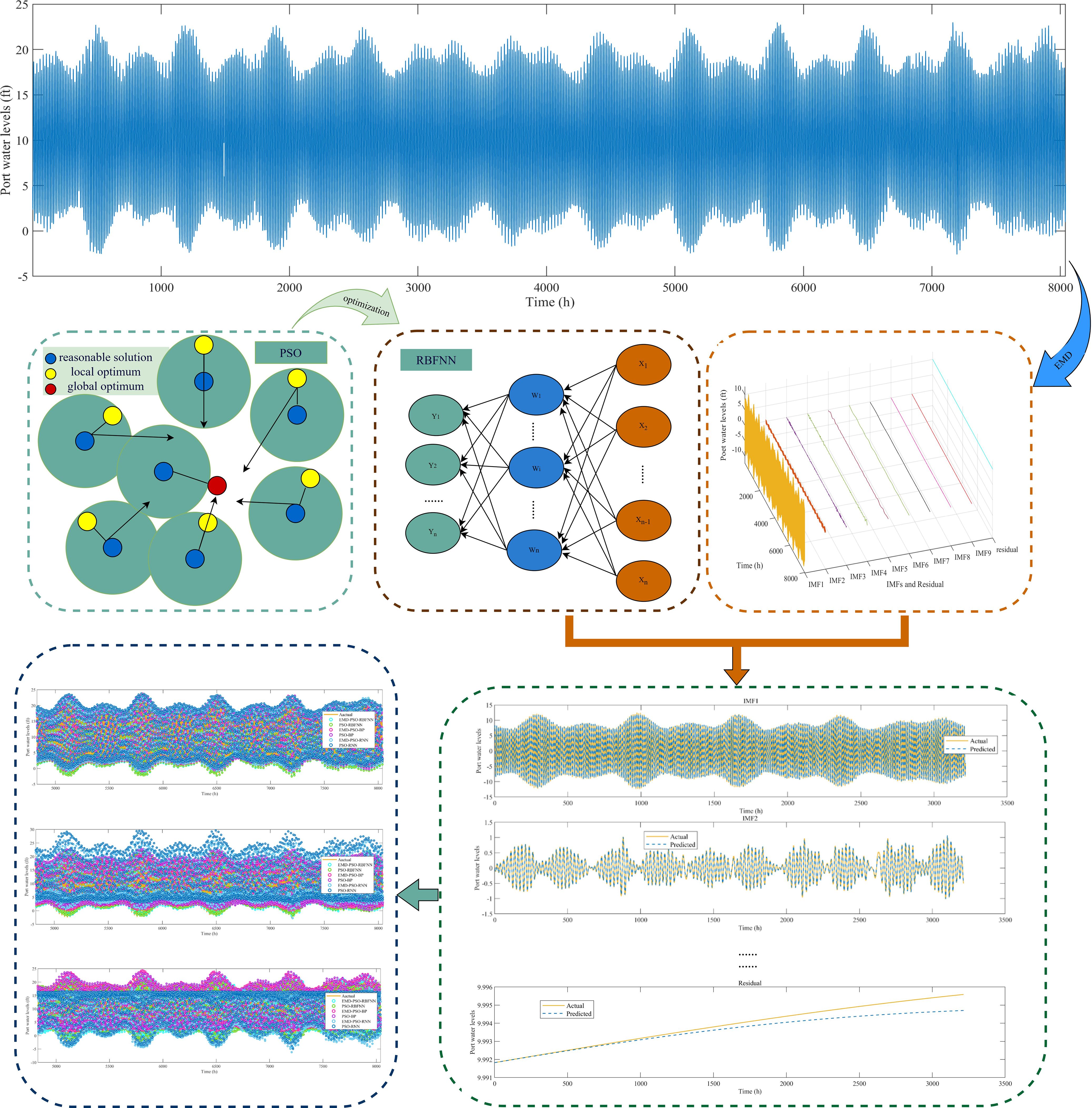
Figure 1. Model prediction process proposed in the paper.

3 Data description and processing

3.1 Data description

The data used in this study were sourced from the water levels of four U.S. ports: Port Angeles, Port Townsend, Port Isabel, and Eastport. The datasets for these four ports include hourly water level measurements from January 1, 2021, to December 1, 2021, with a total of 8,040 data samples per port. Table 1 presents the detailed geographical information of the four datasets’ corresponding ports used in this study. The water level variations for Port Angeles, Port Townsend, Port Isabel, and Eastport are shown in Figure 2.

Table 1

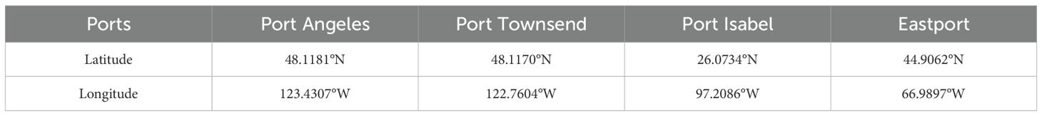
Table 1. Geographical information of each port.

Figure 2

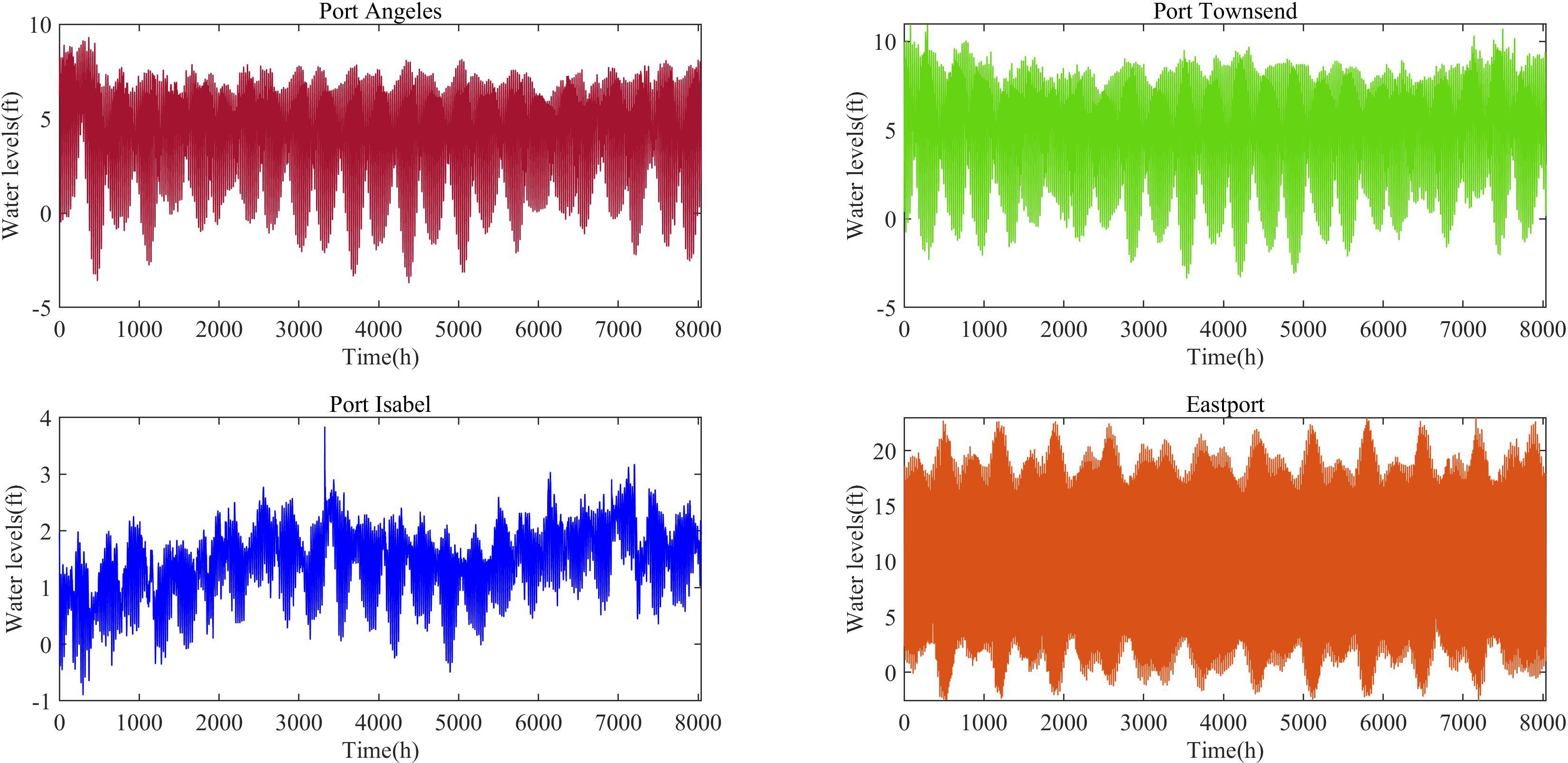
Figure 2. Changes in water levels at various ports.

3.2 Data preprocessing

EMD was used to decompose and preprocess the water levels of Port Angeles, Port Townsend, Port Isabel, and Eastport, obtaining the low-frequency non-linear subsequences. Specifically, the decomposition of Port Angeles yielded eight IMFs and one residual, Port Townsend yielded eight IMFs and one residual, Port Isabel yielded nine IMFs and one residual, and Eastport yielded nine IMFs and one residual. The decomposition of the water level sequences for each port using EMD is shown in Figure 3. By comparing the original signals in Figure 2 with the subsequences obtained from the decomposition, it is evident that the non-linearity of the IMFs and residuals significantly decreased.

Figure 3

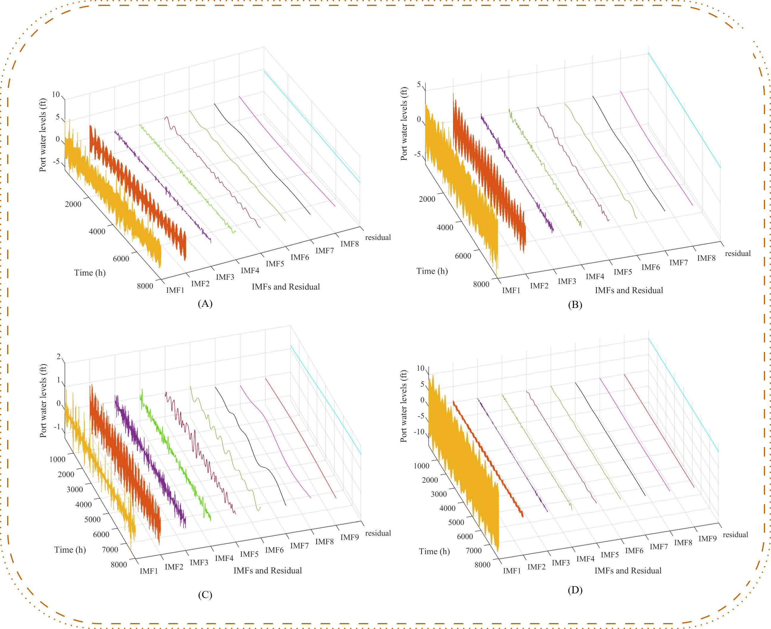
Figure 3. EMD decomposition of water level time series at various ports. (A) Port Angeles, (B) Port Townsend, (C) Port Isabel, and (D) Eastport. EMD, empirical mode decomposition.

3.3 Prediction error analysis

To thoroughly assess the model’s effectiveness in predicting port water levels, several evaluation metrics were used, including mean absolute percentage error (MAPE), mean squared error (MSE), root mean squared error (RMSE), normalized root mean squared error (NRMSE), mean absolute error (MAE), and the coefficient of determination (R²). Among these, smaller values of MAPE, MSE, RMSE, NRMSE, and MAE indicate better prediction performance, while an R² value approaching 1 demonstrates higher prediction reliability. The formulas for each evaluation metric are as follows:

$\begin{array}{ll}MAPE=\frac{100\%}{n}{\displaystyle \sum _{i=1}^n\left|\frac{\widehat{y_i}-y_i}{y_i}\right|}& (14)\end{array}$

$\begin{array}{ll}MSE=\frac{1}{n}{\displaystyle \sum _{i=1}^n{(y_i-{\widehat{y}}_i)}^2}& (15)\end{array}$

$\begin{array}{ll}RMSE=\sqrt{\frac{1}{n}{\displaystyle \sum _{i=1}^n{(y_i-\widehat{y_i})}^2}}& (16)\end{array}$

$\begin{array}{ll}NRMSE=\sqrt{\frac{1}{n}{\displaystyle \sum _{i=1}^n{(y_i-\widehat{y_i})}^2}}/[\max (y)-\min (y)]& (17)\end{array}$

$\begin{array}{ll}MAE=\frac{1}{n}{\displaystyle \sum _{i=1}^n|y_i-\widehat{y_i}|}& (18)\end{array}$

$\begin{array}{ll}{R}^2=1-{{\displaystyle \sum _{i=1}^n(y_i-\widehat{y_i})}}^2/{{\displaystyle \sum _{i-1}^n(y_i-\overline{y})}}^2& (19)\end{array}$

where $y_i$ represents the actual value at a given time i, $\widehat{y_i}$ denotes the predicted value at the same time i, n indicates the total number of predicted data points, and $\overline{y}$ refers to the mean of the data.

4 Simulation testing and analysis of results

In this study, the first 4,824 hours of the water level data from Port Angeles, Port Townsend, Port Isabel, and Eastport were used as the training data and the subsequent 3,216 hours as the testing data, with a 6:4 ratio for the training and testing datasets. The PSO parameters were set as follows: $\omega =0.5$, $c_1=1$, and $c_2=1$ with a particle population size of 100 and a maximum number of iterations set to 100. Considering that ship operations entering and leaving the port require prior notification to the port authorities, the prediction time step for the model was configured to 6 hours. A multi-step prediction comparison was conducted using Eastport as an example. The simulations were executed in MATLAB 2019b.

Ship operations entering and leaving ports typically require prior notification to port authorities. Therefore, a 6-hour lead time was adopted to predict water levels, and comparisons were made for the results at Port Angeles, Port Townsend, and Port Isabel. Figures 4–6 present the water level prediction results and the comparisons between the PSO-RBFNN model and the EMD-PSO-RBFNN model for these three ports.

Figure 4

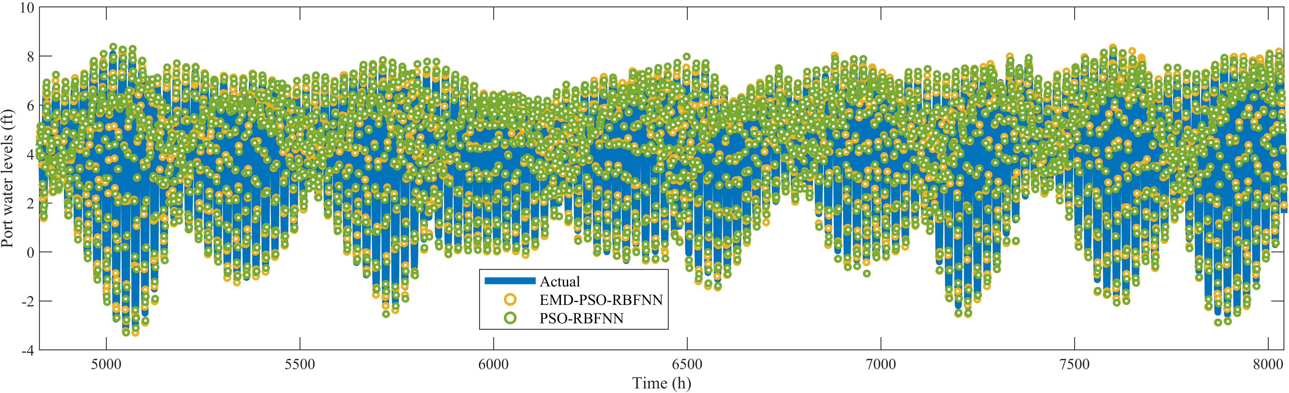
Figure 4. Comparison of PSO-RBFNN and EMD-PSO-RBFNN prediction results for Port Angeles. PSO, particle swarm optimization; RBFNN, radial basis function neural network; EMD, empirical mode decomposition.

Figure 5

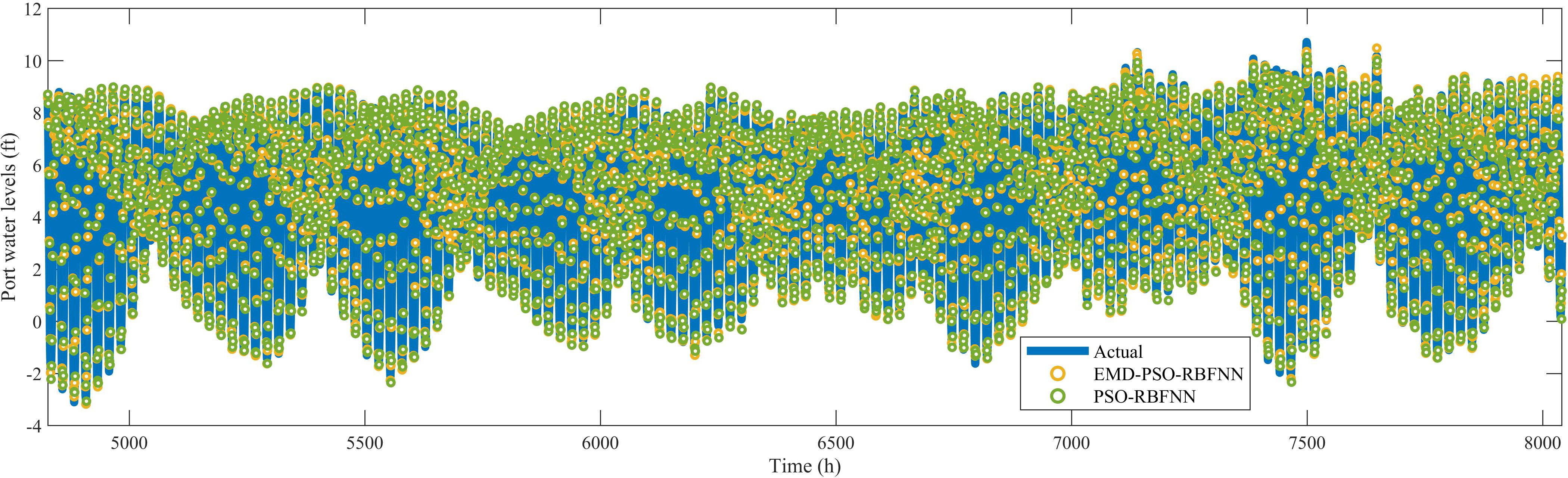
Figure 5. Comparison of PSO-RBFNN and EMD-PSO-RBFNN prediction results for Port Townsend. PSO, particle swarm optimization; RBFNN, radial basis function neural network; EMD, empirical mode decomposition.

Figure 6

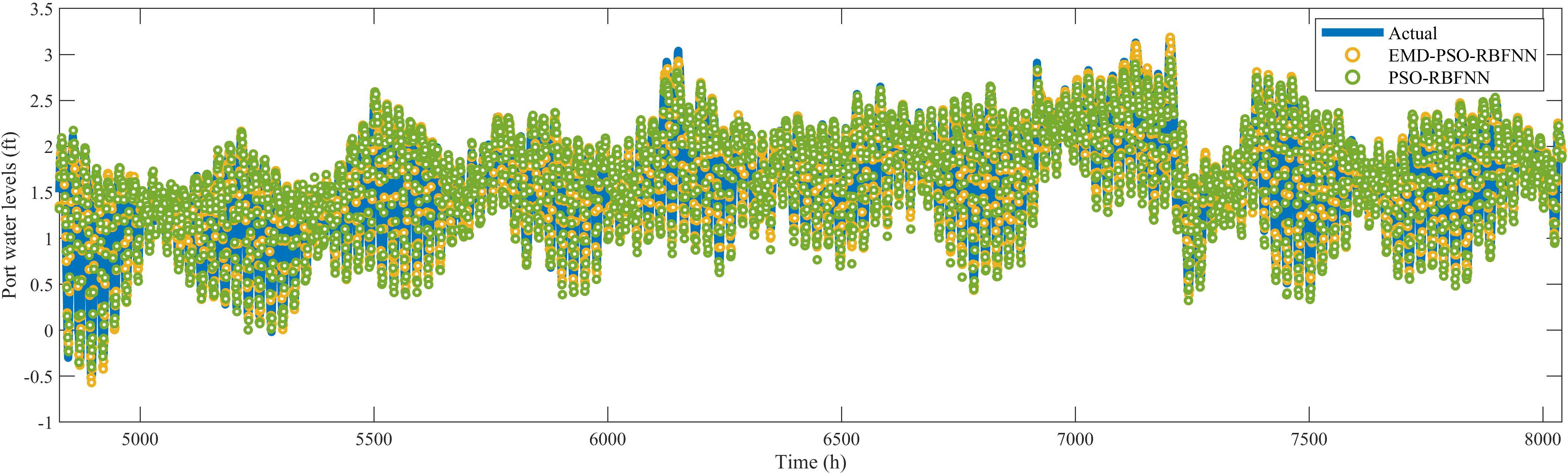
Figure 6. Comparison of PSO-RBFNN and EMD-PSO-RBFNN prediction results for Port Isabel. PSO, particle swarm optimization; RBFNN, radial basis function neural network; EMD, empirical mode decomposition.

From Figures 4–6, it can be observed that the PSO-RBFNN model already provides satisfactory prediction results for port water levels. However, the EMD-enhanced model demonstrated even greater prediction accuracy. For instance, in Figure 6, during data points 7126–7135 (corresponding to 2021/10/24, 21:00 to 2021/10/25, 6:00), the EMD-PSO-RBFNN model produced prediction results that exhibit higher accuracy when compared to actual values. In contrast, the PSO-RBFNN model showed limitations in its prediction capability, particularly under extreme water level conditions. This indicates that EMD enhanced the model’s prediction performance, thereby improving the accuracy of the PSO-RBFNN model.

To demonstrate the convergence performance of PSO in optimizing the RBFNN model, the iterations of PSO during the prediction process of subsequences for Port Angeles were analyzed, as shown in Figure 7.

Figure 7

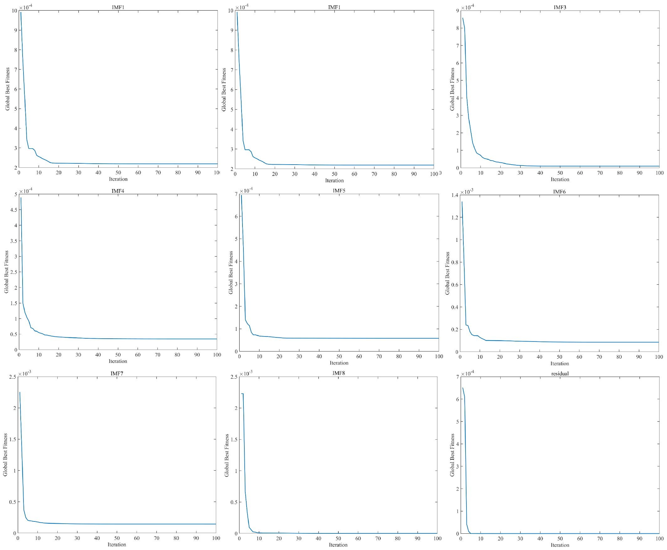
Figure 7. PSO optimization convergence curves in Port Angeles water level prediction. PSO, particle swarm optimization.

By analyzing the convergence curves in Figure 7, it is evident that PSO demonstrated both normal and efficient optimization performance for each subsequence during the forecasting process. Most components achieved rapid convergence within 10–30 iterations, with fitness values quickly stabilizing and showing no significant oscillations or fluctuations. This indicates that the particle swarm performed stably during the local search phase, without falling into local optima or encountering other convergence issues.

The results of the convergence curves further show that PSO can effectively reduce the fitness value to an extremely low level, thereby confirming its significant contribution to improving the accuracy of water level predictions. The automatic parameter adjustment capability of PSO not only highlights its efficiency and intelligent characteristics but also enables rapid convergence to near-optimal solutions. Throughout the entire model, PSO plays a core optimization role, significantly enhancing the model’s performance and providing strong technical support for the development of a high-accuracy water level forecasting model.

To verify the proposed model’s effectiveness in port water level prediction, a backpropagation (BP) neural network (Chen and Zeng, 2013), known for its strong non-linear mapping capability and optimization of network weights and biases via the error backpropagation algorithm, and a recurrent neural network (RNN) (Lu and Xu, 2024), proficient in handling sequential data and capturing more subtle relationships and patterns, were selected for comparison. The PSO-BP, PSO-RNN, EMD-PSO-BP, and EMD-PSO-RNN models were constructed and employed for port water level prediction under the same conditions for comparative analysis with the proposed model. Figure 8 presents a visual comparison of the evaluation metrics for water level prediction across the three ports and all models, while Table 2 provides a comprehensive numerical analysis of the prediction errors.

Figure 8

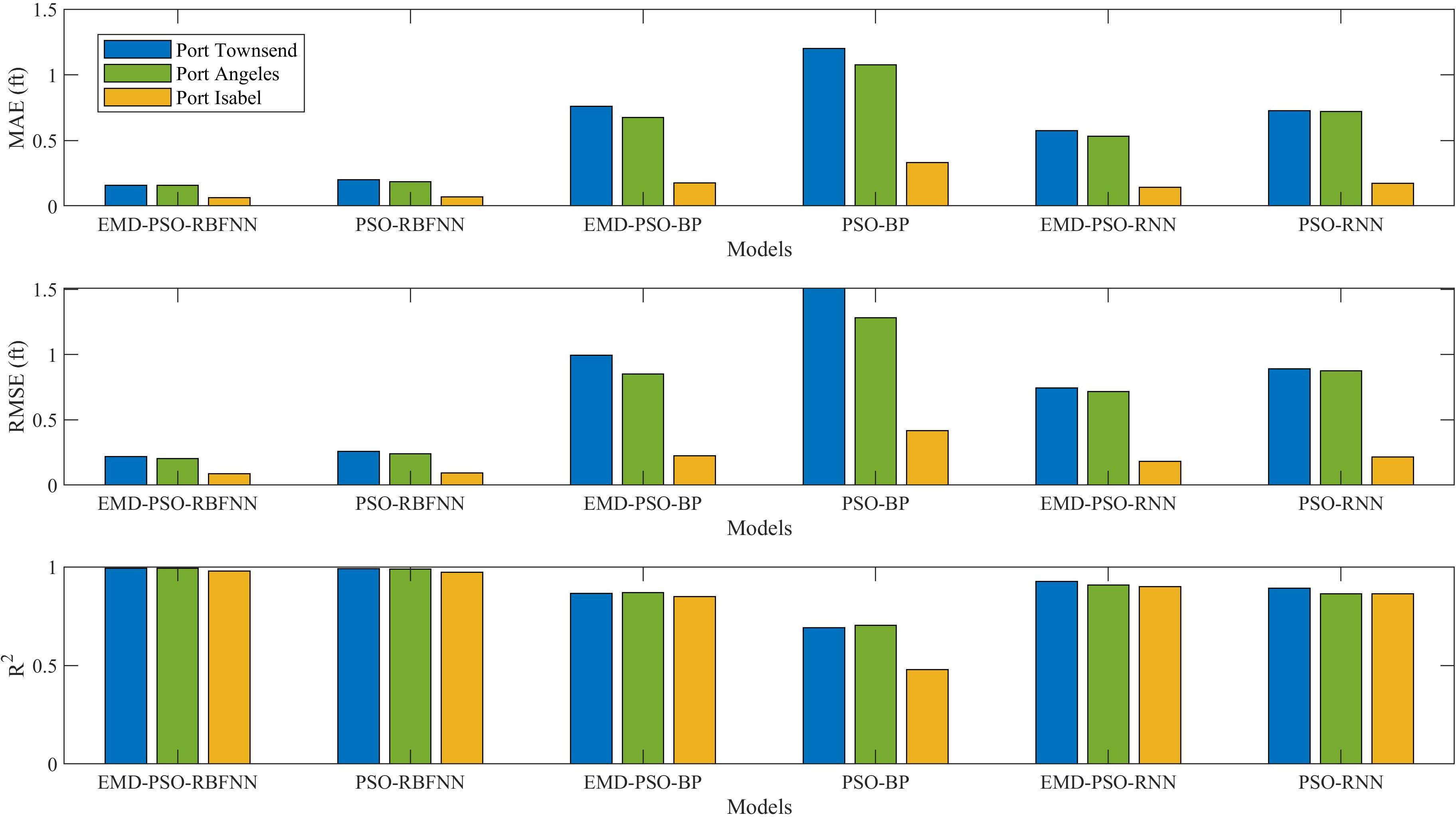
Figure 8. Visualization of prediction errors for water levels across three ports using different models.

Table 2

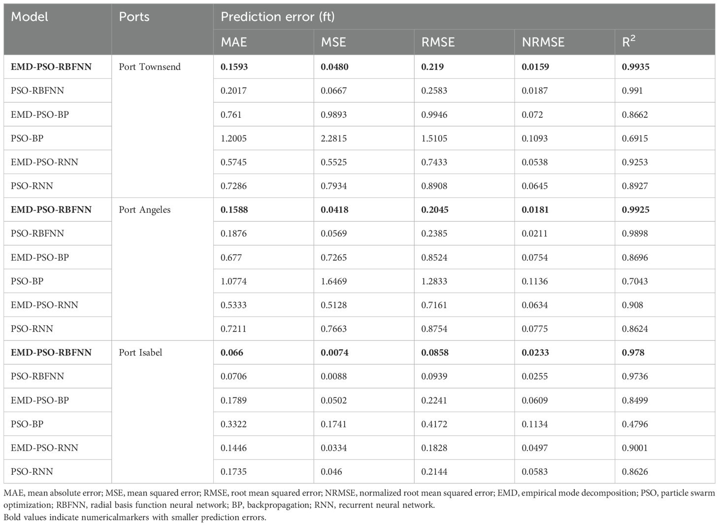
Table 2. Comparison of prediction errors for port water levels 6 hours in advance across different models.

From Figure 8, it can be visually observed that among all models, the EMD-PSO-RBFNN demonstrated the best prediction performance for the water levels of the three ports. The prediction accuracy of the PSO-RBFNN, PSO-BP, and PSO-RNN models improved under the enhancement of EMD. Table 2 presents a comprehensive numerical comparison of water level prediction errors at Port Angeles, Port Townsend, and Port Isabel across all models. As shown in Table 2, the EMD-PSO-RBFNN achieved superior performance in every prediction evaluation metric compared to other models. Notably, for the water level prediction of Port Angeles and Port Townsend, the R² values were 0.9935 and 0.9925, respectively, which were very close to 1. For the water level prediction of Port Isabel, the evaluation metrics MAE, MSE, RMSE, and NRMSE exhibited significantly low error values at 0.066, 0.0074, 0.0858, and 0.0233, respectively. The PSO-BP model showed relatively poor prediction performance for the water levels at the three ports. However, under the enhancement of EMD, its prediction performance improved significantly. For example, the R² values of the EMD-PSO-BP model increased by 20.2%, 19%, and 43.6% compared to the PSO-BP model for Port Angeles, Port Townsend, and Port Isabel, respectively. The PSO-RNN model performed moderately for water level prediction at the three ports, but its performance improved considerably after EMD enhancement. These results indicate that EMD effectively reduced prediction errors.

In previous studies, multi-step prediction has rarely been considered due to its inefficiency and lack of accuracy. However, multi-step prediction is crucial in practical applications (Bai and Xu, 2021). For multi-step prediction, the prediction error tends to increase as the prediction horizon extends. Therefore, it is essential to evaluate the prediction horizon within an acceptable accuracy range, as the choice of horizon has a significant impact on the results. In this study, Eastport was used as an example to perform forecasts with lead times of 6 hours, 12 hours, and 24 hours to validate the prediction performance of various models. The multi-step prediction results of EMD-PSO-RBFNN, PSO-RBFNN, EMD-PSO-BP, PSO-BP, EMD-PSO-RNN, and PSO-RNN for Eastport water levels are compared in Figures 9–11.

Figure 9

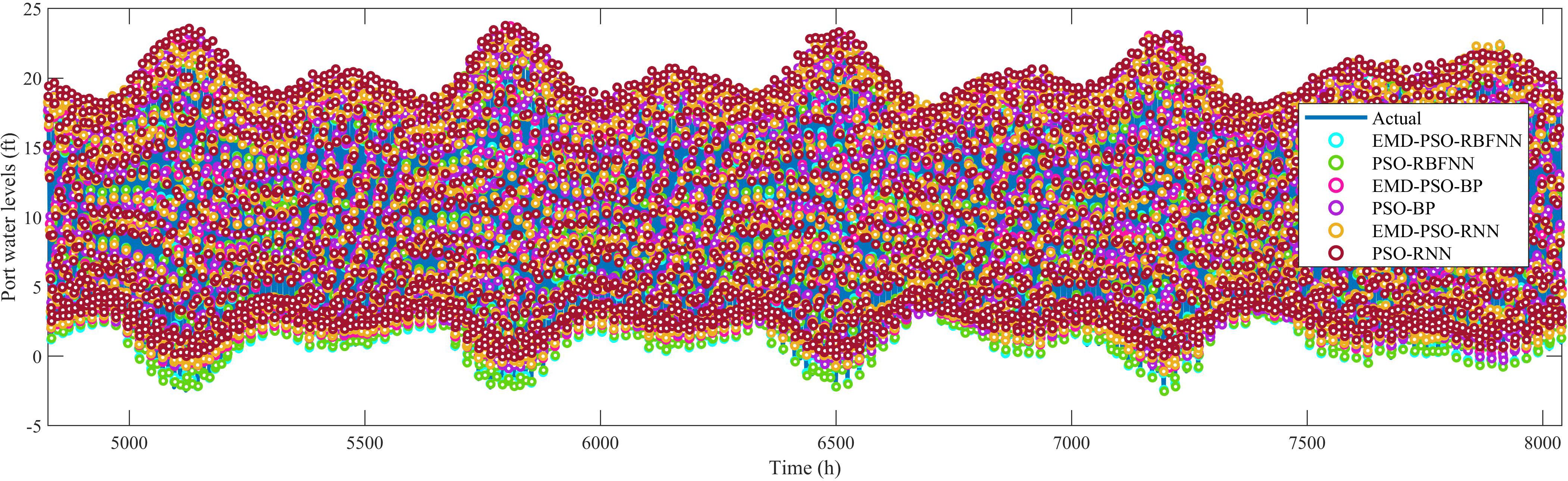
Figure 9. Comparison of 6-hour-ahead water level predictions for Eastport across different models.

Figure 10

Figure 10. Comparison of 12-hour-ahead water level predictions for Eastport across different models.

Figure 11

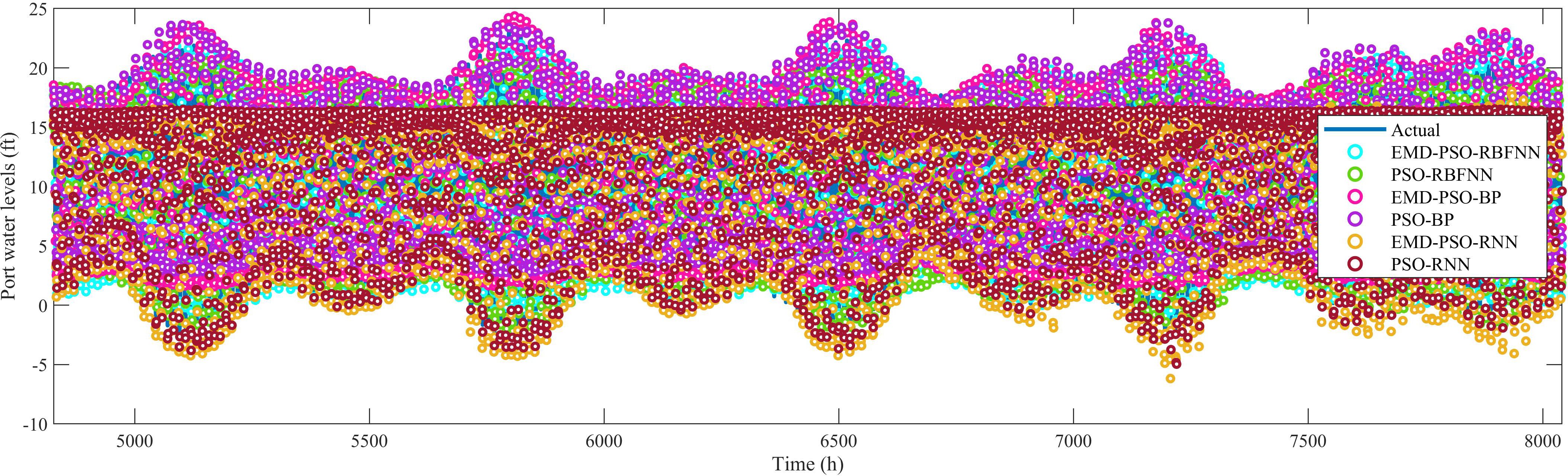
Figure 11. Comparison of 24-hour-ahead water level predictions for Eastport across different models.

From Figures 9–11, it can be observed that EMD effectively improved the prediction performance of PSO-RBFNN, PSO-BP, and PSO-RNN under different prediction horizons. Both EMD-PSO-RBFNN and PSO-RBFNN demonstrated stable prediction performance, with their predicted results remaining close to the actual values over increasing prediction horizons. In contrast, the deviations between the predicted results and actual values for EMD-PSO-RNN and PSO-RNN gradually increased as the prediction horizon extended. For EMD-PSO-BP and PSO-BP, the deviations became more significant when the prediction horizon was extended to 24 hours. The related prediction evaluation metrics for each model were compared and are presented in Figure 12, and the detailed numerical comparison of prediction errors is presented in Table 3.

Figure 12

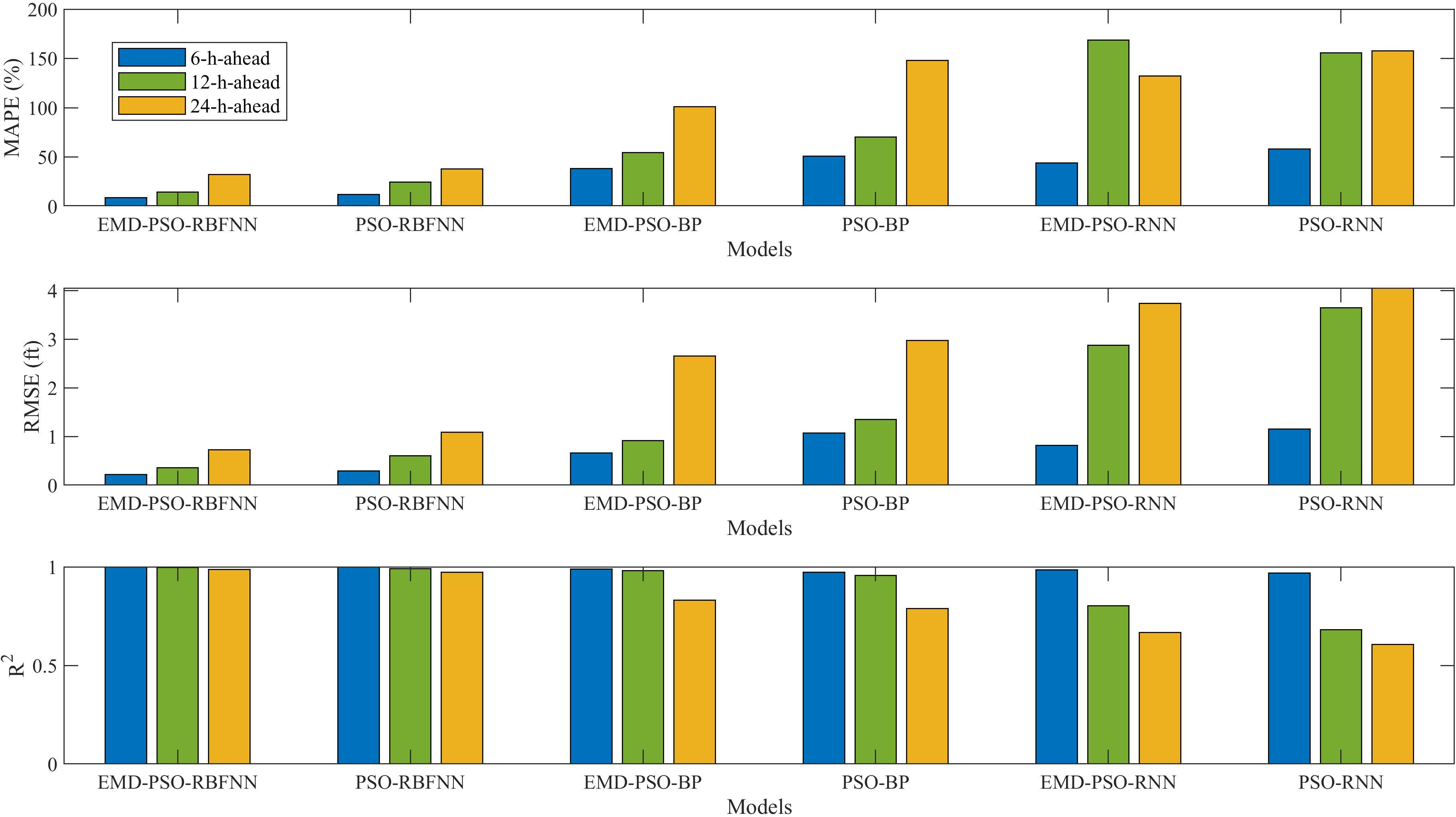
Figure 12. Visualization of prediction errors for Eastport water levels at different lead times across models.

Table 3

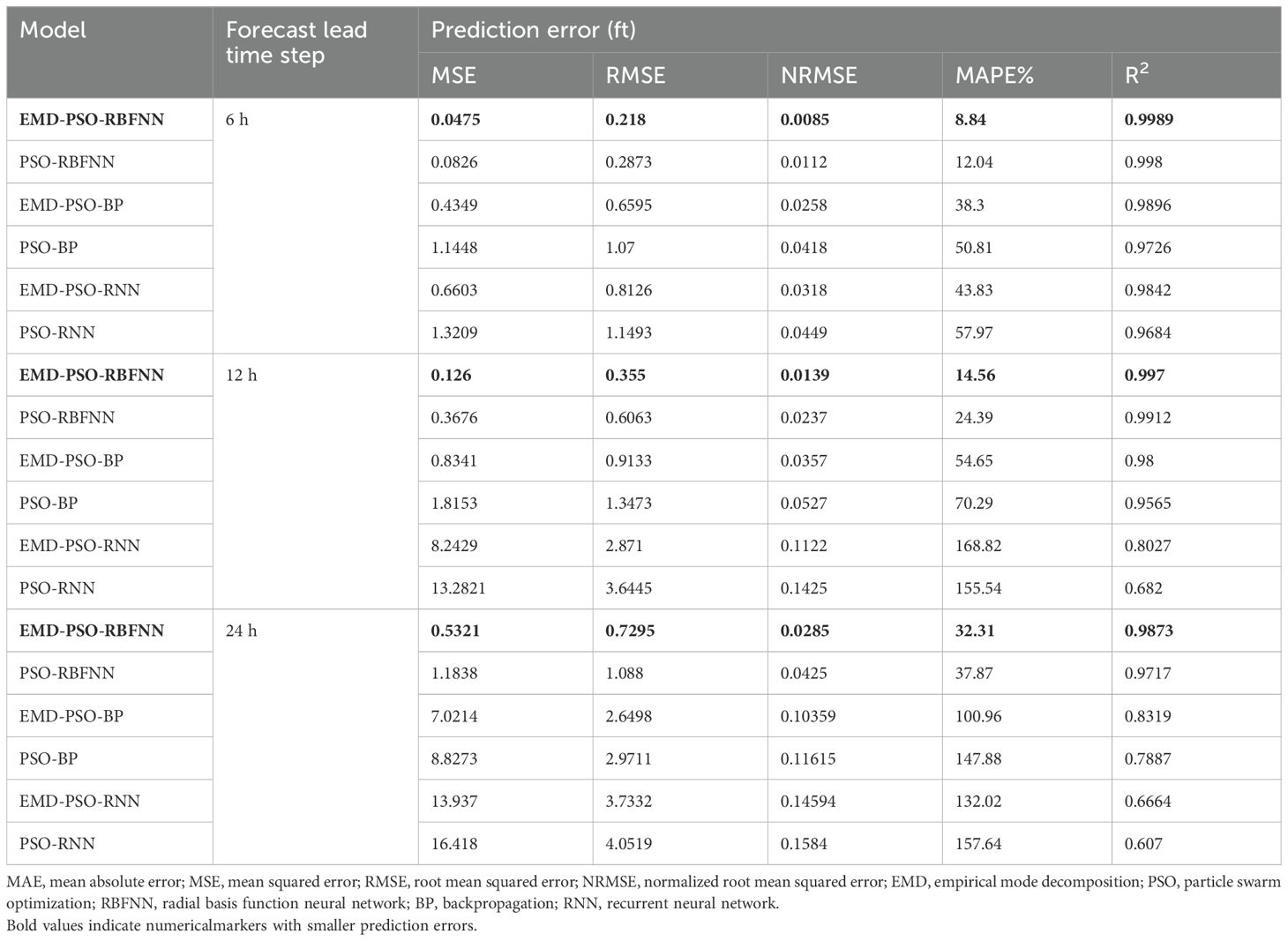
Table 3. Detailed numerical comparison of prediction errors for Eastport water levels at different lead times across models.

From the comparison in Figure 12, Table 3, it can be observed that the prediction error of all models increased as the prediction horizon extended. PSO-RBFNN and EMD-PSO-RBFNN achieved favorable results across different prediction horizons. However, the prediction errors of EMD-PSO-RBFNN were consistently lower than those of PSO-RBFNN, indicating an improvement in prediction accuracy over the PSO-RBFNN model. EMD-PSO-BP and PSO-BP performed well for prediction horizons of 6 hours and 12 hours, but their prediction accuracy declined significantly for a 24-hour horizon. For instance, the MAPE values of EMD-PSO-BP and PSO-BP for a 24-hour prediction were 62.66% and 97.07% lower, respectively, compared to their 6-hour prediction. However, under the enhancement of EMD, EMD-PSO-BP consistently outperformed PSO-BP across different prediction horizons. For example, for a 24-hour forecast, the R² of EMD-PSO-BP improved by 5.19% compared to PSO-BP. EMD-PSO-RNN and PSO-RNN demonstrated good performance for a 6-hour prediction but exhibited poor prediction accuracy for 12-hour and 24-hour horizons. In particular, their MAE, MSE, and MAPE values showed significant errors, and the R² values remained below 0.85 for these longer horizons.

The proposed EMD-PSO-RBFNN model in this study demonstrated satisfactory performance in the prediction of port water levels. Its effectiveness has been validated through comparisons with the prediction results of other neural network models. Data from four ports were used for verification, and the model achieved favorable results for prediction horizons of 6 hours, 12 hours, and 24 hours. Its long prediction cycle makes it effectively applicable to port operations.

5 Conclusion

To address the non-linearity and the influence of multiple factors on port water level variations, this study proposed an enhanced prediction scheme for port water levels using EMD for data preprocessing and combining PSO with RBFNN. PSO was used to optimize the center and spread parameters of the RBFNN, thereby improving the prediction performance of the model. The PSO-RBFNN model was employed to predict the low-non-linearity sub-series obtained from EMD decomposition. This study conducted experiments using water level data from four different ports and performed multi-step prediction to validate the model’s prediction performance. The results showed low errors between the prediction and actual values. Comparisons with other neural network models demonstrated the effectiveness of the EMD-PSO-RBFNN model for the prediction of port water levels. The findings highlight that the proposed model achieved strong performance in port water level prediction, enabling real-time monitoring of water level variations and enhancing port operational safety. In the future, we aim to incorporate more factors influencing water level variations, such as storm surges, climate change, and port wastewater discharge, to improve the comprehensiveness of the prediction and adapt to the diversity of port operations while extending the prediction horizon. Additionally, we will explore the potential application of novel intelligent optimization methods in prediction models.

Data availability statement

The original contributions presented in the study are included in the article/supplementary material. Further inquiries can be directed to the corresponding author.

Author contributions

LW: Conceptualization, Funding acquisition, Software, Writing – review & editing. SL: Conceptualization, Data curation, Methodology, Writing – original draft, Writing – review & editing. SW: Formal analysis, Project administration, Resources, Supervision, Validation, Writing – review & editing. JY: Methodology, Project administration, Supervision, Writing – review & editing. RL: Conceptualization, Formal analysis, Validation, Writing – review & editing. JG: Data curation, Investigation, Writing – review & editing.

Funding

The author(s) declare financial support was received for the research, authorship, and/or publication of this article. This research was funded by the National Science Foundation of China, grant number 52171346 and grant number 52271361; the Fund of Guangdong Provincial Key Laboratory of Intelligent Equipment for South China Sea Marine Ranching, grant number 2023B1212030003; and Key Area Project of Ordinary Universities in Guangdong Province, grant number 2024ZDZX3054.

Acknowledgments

We are sincerely grateful to the many teachers, friends, and classmates who generously shared their valuable inputs as we finalized this study. In addition, we would like to express our sincere gratitude to the university we are currently attending for encouraging us to be innovative and enterprising and for providing us with a platform and opportunity to combine theory and practice.

Conflict of interest

The authors declare that the research was conducted in the absence of any commercial or financial relationships that could be construed as a potential conflict of interest.

Generative AI statement

The author(s) declare that no Generative AI was used in the creation of this manuscript.

Publisher’s note

All claims expressed in this article are solely those of the authors and do not necessarily represent those of their affiliated organizations, or those of the publisher, the editors and the reviewers. Any product that may be evaluated in this article, or claim that may be made by its manufacturer, is not guaranteed or endorsed by the publisher.

References

Adnan R. M., Sadeghifar T., Alizamir M., Azad M. T., Makarynskyy O., Kisi O., et al. (2023). Short-term probabilistic prediction of significant wave height using bayesian model averaging: Case study of chabahar port, Iran. Ocean Eng. 272, 113887. doi: 10.1016/j.oceaneng.2023.113887

Crossref Full Text | Google Scholar

Appell G., Mero T., Bethem T., French G. (1994). The development of a real-time port information system. IEEE J. oceanic Eng. 19, 149–157. doi: 10.1109/48.286636

Crossref Full Text | Google Scholar

Bai L.-H., Xu H. (2021). Accurate estimation of tidal level using bidirectional long short-term memory recurrent neural network. Ocean Eng. 235, 108765. doi: 10.1016/j.oceaneng.2021.108765

Crossref Full Text | Google Scholar

Cao L.-s., Zhu J. (2014). Prediction of submarine hydrodynamics using CFD-based calculations and RBF neural network. J. Ship Mech. 18, (3). doi: 10.3969/j.issn.1007-7294.2014.03.002

Crossref Full Text | Google Scholar

Chen H., Zeng Z. (2013). Deformation prediction of landslide based on improved back-propagation neural network. Cogn. Comput. 5, 56–62. doi: 10.1007/s12559-012-9148-1

Crossref Full Text | Google Scholar

Christodoulou A., Christidis P., Demirel H. (2019). Sea-level rise in ports: a wider focus on impacts. Maritime Economics Logistics 21, 482–496. doi: 10.1057/s41278-018-0114-z

Crossref Full Text | Google Scholar

Dehdarinejad E., Bayareh M. (2023). Performance analysis of a novel cyclone separator using RBFNN and MOPSO algorithms. Powder Technol. 426, 118663. doi: 10.1016/j.powtec.2023.118663

Crossref Full Text | Google Scholar

Deng B., Liu P., Chin R. J., Kumar P., Jiang C., Xiang Y., et al. (2022). Hybrid metaheuristic machine learning approach for water level prediction: A case study in Dongting Lake. Front. Earth Sci. 10. doi: 10.3389/feart.2022.928052

Crossref Full Text | Google Scholar

Deo R. C., Şahin M. (2016). An extreme learning machine model for the simulation of monthly mean streamflow water level in eastern Queensland. Environ. Monit. Assess. 188, 1–24. doi: 10.1007/s10661-016-5094-9

PubMed Abstract | Crossref Full Text | Google Scholar

Dong S., Chen C., Tao S., Gao J. (2018). Stochastic model for estimating extreme water level in port and coastal engineering design. J. Ocean Univ. China 17, 744–752. doi: 10.1007/s11802-018-3558-y

Crossref Full Text | Google Scholar

Feng D., Li Y., Liu J., Liu Y. (2024). A particle swarm optimization algorithm based on modified crowding distance for multimodal multi-objective problems. Appl. Soft Computing 152, 111280. doi: 10.1016/j.asoc.2024.111280

Crossref Full Text | Google Scholar

Gao J., Shi H., Zang J., Liu Y. (2023). Mechanism analysis on the mitigation of harbor resonance by periodic undulating topography. Ocean Eng. 281, 114923. doi: 10.1016/j.oceaneng.2023.114923

Crossref Full Text | Google Scholar

Ghorbani M. A., Deo R. C., Karimi V., Yaseen Z. M., Terzi O. (2018). Implementation of a hybrid MLP-FFA model for water level prediction of Lake Egirdir, Turkey. Stochastic Environ. Res. 32, 1683–1697. doi: 10.1007/s00477-017-1474-0

Crossref Full Text | Google Scholar

Gracia V., Sierra J. P., Gómez M., Pedrol M., Sampé S., García-León M., et al. (2019). Assessing the impact of sea level rise on port operability using LiDAR-derived digital elevation models. Remote Sens. Environ. 232, 111318. doi: 10.1016/j.rse.2019.111318

Crossref Full Text | Google Scholar

Han X. (2021). Ship traffic flow prediction based on fractional order gradient descent with momentum for RBF neural network. J. Ship Res. 65, 100–107. doi: 10.5957/JOSR.08190052

Crossref Full Text | Google Scholar

Hao W., Sun X., Wang C., Chen H., Huang L. (2022). A hybrid EMD-LSTM model for non-stationary wave prediction in offshore China. Ocean Eng. 246, 110566. doi: 10.1016/j.oceaneng.2022.110566

Crossref Full Text | Google Scholar

Huang N. E., Shen Z., Long S. R., Wu M. C., Shih H. H., Zheng Q., et al. (1998). The empirical mode decomposition and the Hilbert spectrum for nonlinear and non-stationary time series analysis. Proc. R. Soc. London. Ser. A: mathematical Phys. Eng. Sci. 454, 903–995. doi: 10.1098/rspa.1998.0193

PubMed Abstract | Crossref Full Text | Google Scholar

Huo D., Chen J., Zhang H., Shi Y., Wang T. (2023). Intelligent prediction for digging load of hydraulic excavators based on RBF neural network. Measurement 206, 112210. doi: 10.1016/j.measurement.2022.112210

Crossref Full Text | Google Scholar

Juan N. P., Matutano C., Valdecantos V. N. (2023). Uncertainties in the application of artificial neural networks in ocean engineering. Ocean Eng. 284, 115193. doi: 10.1016/j.oceaneng.2023.115193

Crossref Full Text | Google Scholar

Kennedy J., Eberhart R. (1995). Particle swarm optimization, Proceedings of ICNN’95-international conference on neural networks. ieee 4, 1942–1948. doi: 10.1109/ICNN.1995.488968

Crossref Full Text | Google Scholar

Kumar N. K., Savitha R., Al Mamun A. (2017). Regional ocean wave height prediction using sequential learning neural networks. Ocean Eng. 129, 605–612. doi: 10.1016/j.oceaneng.2016.10.033

Crossref Full Text | Google Scholar

López J. C. S., Pina G. G. (1988). Long waves in a Spanish harbour. Coast. Eng. 984–998. doi: 10.1061/9780872626874.074

Crossref Full Text | Google Scholar

López M., Iglesias G., Kobayashi N. (2012). Long period oscillations and tidal level in the Port of Ferrol. Appl. Ocean Res. 38, 126–134. doi: 10.1016/j.apor.2012.07.006

Crossref Full Text | Google Scholar

López M., Iglesias G. J. (2013). Artificial intelligence for estimating infragravity energy in a harbour. Ocean Eng. 57, 56–63. doi: 10.1016/j.oceaneng.2012.08.009

Crossref Full Text | Google Scholar

Lu M., Xu X. (2024). TRNN: An efficient time-series recurrent neural network for stock price prediction. Inf. Sci. 657, 119951. doi: 10.1016/j.ins.2023.119951

Crossref Full Text | Google Scholar

Nur F., Marufuzzaman M., Puryear S. M. (2020). Optimizing inland waterway port management decisions considering water level fluctuations. Comput. Ind. Eng. 140, 106210. doi: 10.1016/j.cie.2019.106210

Crossref Full Text | Google Scholar

Rabinovich A. B. (2010). Seiches and harbor oscillations, Handbook of coastal and ocean engineering. World Sci., 193–236. doi: 10.1142/9789812819307_0009

Crossref Full Text | Google Scholar

Ruiz-Aguilar J. J., Turias I., Gonzalez-Enrique J., Urda D., Elizondo D. (2021). A permutation entropy-based EMD-ANN forecasting ensemble approach for wind speed prediction. Neural Computing Appl. 33, 2369–2391. doi: 10.1007/s00521-020-05141-w

Crossref Full Text | Google Scholar

Song T., Wang J., Huo J., Wei W., Han R., Xu D., et al. (2023). Prediction of significant wave height based on EEMD and deep learning. Front. Mar. Sci. 10. doi: 10.3389/fmars.2023.1089357

Crossref Full Text | Google Scholar

Tao J., Yu Z., Zhang R., Gao F. (2021). RBF neural network modeling approach using PCA based LM-GA optimization for coke furnace system. Appl. Soft Computing 111, 107691. doi: 10.1016/j.asoc.2021.107691

Crossref Full Text | Google Scholar

Ulm M., Arns A., Wahl T., Meyers S. D., Luther M. E., Jensen J. (2016). The impact of a Barrier Island loss on extreme events in the Tampa Bay. Front. Mar. Sci. 3. doi: 10.3389/fmars.2016.00056

Crossref Full Text | Google Scholar

Wang L., Liao S., Wang S., Jia B., Yin J., Li R. (2024). Real-time prediction of metacentric height of ro-ro passenger ships in Qiongzhou strait based on improved RBF neural network. Ocean Eng. 312, 119067. doi: 10.1016/j.oceaneng.2024.119067

Crossref Full Text | Google Scholar

Xu D., Yin J. (2024). An enhanced hybrid scheme for ship roll prediction using support vector regression and TVF-EMD. Ocean Eng. 307, 117951. doi: 10.1016/j.oceaneng.2024.117951

Crossref Full Text | Google Scholar

Yang J., Zhang T., Zhang J., Lin X., Wang H., Feng T. (2024). A ConvLSTM nearshore water level prediction model with integrated attention mechanism. Front. Mar. Sci. 11, 116297. doi: 10.3389/fmars.2024.1470320

Crossref Full Text | Google Scholar

Yin J.-C., Perakis A. N., Wang N. (2018). A real-time ship roll motion prediction using wavelet transform and variable RBF network. Ocean Eng. 160, 10–19. doi: 10.1016/J.OCEANENG.2018.04.058

Crossref Full Text | Google Scholar

Yin J.-C., Wang N.-N., Hu J.-Q. (2015). A hybrid real-time tidal prediction mechanism based on harmonic method and variable structure neural network. Eng. Appl. Artif. Intell. 41, 223–231. doi: 10.1016/j.engappai.2015.03.002

Crossref Full Text | Google Scholar

Yin J., Wang H., Wang N., Wang X. (2023). An adaptive real-time modular tidal level prediction mechanism based on EMD and Lipschitz quotients method. Ocean Eng. 289. doi: 10.1016/j.oceaneng.2023.116297

Crossref Full Text | Google Scholar

Zhang C., Zhang R., Zhu Z., Song X., Su Y., Li G., et al. (2023). Bottom hole pressure prediction based on hybrid neural networks and Bayesian optimization. Petroleum Sci. 20, 3712–3722. doi: 10.1016/j.petsci.2023.07.009

Crossref Full Text | Google Scholar

Zheng Z., Ma X., Huang X., Ma Y., Dong G. (2022). Wave forecasting within a port using WAVEWATCH III and artificial neural networks. Ocean Eng. 255, 111475. doi: 10.1016/j.oceaneng.2022.111475

Crossref Full Text | Google Scholar