Canopy-forming kelp forests persist in the dynamic subregion of the Broughton Archipelago, British Columbia, Canada

Canopy-forming kelp forests act as foundation species that provide a wide range of ecosystem services along temperate coastlines. With climate change, these ecosystems are experiencing changing environmental and biotic conditions; however, the kelp distribution and drivers of change in British Columbia remain largely unexplored. This research aimed to use satellite imagery and environmental data to investigate the spatiotemporal persistence and resilience of kelp forests in a dynamic subregion of cool ocean temperatures and high kelp abundance in the Broughton Archipelago, British Columbia. The specific objectives were to identify: 1) long-term (1984 to 2023) and short-term (2016 to 2023) kelp responses to environmental changes; and 2) spatial patterns of kelp persistence. The long-term time series was divided into three climate periods: 1984 to 1998, 1999 to 2014, and 2014 to 2023. The first transition between these periods represented a shift into cooler regional sea-surface temperatures and a negative Pacific Decadal Oscillation in 1999. The second transition represented a change into warmer temperatures (with more marine heatwaves and El Niño conditions) after 2014. In the long-term time series (1984 to 2023), which covered a site with Macrocystis pyrifera beds, kelp area increased slightly after the start of the second climate period in 1999. For the short-term time series (2016 to 2023), which focused on eight sites with Nereocystis luetkeana beds, most sites either did not change significantly or expanded in kelp area. This suggests that kelp areas remained persistent across these periods despite showing interannual variability. Thus, the dynamic subregion of the Broughton Archipelago may be a climate refuge for kelps, likely due to cool water temperatures that remain below both species’ upper thermal limits. Spatially, on a bed level, both species were more persistent in the center of the kelp beds, but across the subregion, Macrocystis had more persistent areas than Nereocystis, suggesting life history and/or other factors may be impacting these kelp beds differently. These findings demonstrate the spatiotemporal persistence of kelp forests in the dynamic subregion of the Broughton Archipelago, informing the management of kelp forest ecosystems by First Nations and local communities.

1 Introduction

Canopy-forming kelp forests (order Laminariales) are key habitats in temperate marine regions globally (Jayathilake and Costello, 2021) and are vulnerable to climate change impacts (Reed et al., 2016; Smale, 2020; Wernberg et al., 2024), which can potentially disrupt ecosystem functions, such as habitat provision, fisheries production, nutrient cycling, carbon sequestration, and cultural value (Lamy et al., 2020; Eger et al., 2023; Turner, 2001). Kelp distribution and extent are affected by changes in environmental and biotic conditions, including ocean temperature, salinity, exposure, light, nutrient availability, and the abundance of kelp grazers and predators (Jayathilake and Costello, 2021; Springer et al., 2010; Druehl, 1977; Traiger and Konar, 2018; Hollarsmith et al., 2022; Starko et al., 2024a). These conditions are often closely related to temperature in region-specific ways; for example, in the Northeast Pacific Ocean, warmer waters can correlate with lower salinities (Druehl, 1977), poor nutrient availability (Lowman et al., 2022), and ecological regime shifts (Burt et al., 2018; Hamilton et al., 2021). Furthermore, studies have shown how ocean temperatures directly or indirectly drive kelp dynamics (e.g. Jayathilake and Costello, 2021; Gonzalez-Aragon et al., 2024; Hamilton et al., 2020; Bell et al., 2020; Starko et al., 2022; Mora-Soto et al., 2024a, 2024b).

In the Northeast Pacific Ocean, temperature changes can occur at variable time scales, from steady long-term trends or cyclic changes spanning decades or years, to short-term marine heatwaves, affecting the kelp dynamics differently (Cavanaugh et al., 2011; Krumhansl et al., 2016; Levitus et al., 2000; Mora-Soto et al., 2024a; Smith et al., 2024; Wernberg et al., 2024). Since the 1950s, long-term increases in ocean temperatures have primarily been driven by anthropogenic climate change (Cheng et al., 2022) and can drive changes in kelp distribution and area (Beas-Luna et al., 2020; Berry et al., 2021; Mora-Soto et al., 2024a). For instance, Berry et al. (2021) documented a shift in kelp distribution and a 63% decrease in its area coinciding with a 0.7°C sea-surface temperature (SST) increase throughout the 20th century in Puget Sound, Washington. Additionally, ocean temperatures are influenced by cyclic climatic oscillations (Di Lorenzo et al., 2008), such as the El Niño Southern Oscillation (ENSO) (quantified with the Oceanic Niño Index, ONI) and the Pacific Decadal Oscillation (PDO), which are multi-year and decadal modes of climate variability (Di Lorenzo et al., 2008). These oscillations often lead to warming in the Northeast Pacific Ocean when in a positive phase (Di Lorenzo and Mantua, 2016), with consequent changes in kelp responses. For instance, kelp areas decreased after shifting to positive PDO and ONI but rebounded after the oscillations shifted to negative phases in the Strait of Juan de Fuca (Pfister et al., 2018) and the Strait of Georgia (Mora-Soto et al., 2024a); conversely, kelp disappeared after a positive PDO shift in the 1970s and did not rebound afterward in Gray Bay, Haida Gwaii (Gendall et al., submitted).

Furthermore, ocean temperature change can also manifest in the form of short-term marine heat waves (MHWs), which are anomalously warm events (>5 days) with temperatures above the 90th percentile based on a 30-year climatological baseline (Hobday et al., 2016). A higher frequency and magnitude of MHWs have been observed due to climate change (Frölicher et al., 2018) and are generally associated with positive PDO and ONI years (Di Lorenzo and Mantua, 2016), resulting in prolonged, anomalously warm conditions (Bond et al., 2015). Such conditions were present during the Blob of 2014 to 2016, a prolonged MHW (Bond et al., 2015) that devastated kelp forests across the Northeast Pacific Ocean (Bell et al., 2023; Arafeh-Dalmau et al., 2019; Starko et al., 2024; Mora-Soto et al., 2024a, 2024b). Kelp was reduced after the Blob to 60% of its pre-Blob distribution in Barkley Sound (Starko et al., 2022), to 21% of its pre-Blob distribution in the Northern Salish Sea (Mora-Soto et al., 2024b), and to 13% of its historical area in Haida Gwaii (Gendall et al., submitted).

Kelp forest persistence and resilience to ocean warming and climatic oscillations can be characterized in temporal and spatial domains. In this context, persistence refers to the continued existence of kelp forests through time (Connell & Sousa, 1983), and resilience refers to kelps returning to a reference state after a disturbance, such as thermal stress periods (Holling, 1973). Some studies consider kelp persistence and resilience in the temporal domain, including increasing, decreasing, or no change in kelp areas within a specific study site or region (e.g. Cavanaugh et al., 2019; Mora-Soto et al., 2024a, 2024; etc.). Other studies investigate kelp persistence and resilience in the spatial domain, i.e., identifying areas where kelp is often present. (e.g. Schroeder et al., 2020; Hamilton et al., 2020; Cavanaugh et al., 2023; Arafeh-Dalmau et al., 2023). Currently, kelp forests are declining globally (Krumhansl et al., 2016), however, their persistence and resilience to climate change have been spatially variable, with decreases in 38% of the regions, increases in 27% of regions, and no change in 35% of regions (Krumhansl et al., 2016). This variability in persistence and resilience is often due to spatially explicit patterns in environmental and biotic conditions (Smale, 2020; Bell et al., 2023; Starko et al., 2024a), which can influence the amount of stress the kelps directly experience, as well as have implications for adaptation and ecosystem-scale responses to stressors (Starko et al., 2024b). For instance, kelp areas are expanding in the Arctic due to the increase in ice-free areas (Filbee-Dexter et al., 2019), and conversely, are diminishing in subtropical latitudes such as in Baja California due to the increase in ocean temperatures (Cavanaugh et al., 2019; Beas-Luna et al., 2020; Bell et al., 2023). Beyond global-scale variability, this spatially driven variation in kelp persistence and resilience can be observed at a regional scale in British Columbia (BC), Canada. Kelp areas are increasing on the northwest coast of Vancouver Island where keystone predators (sea otters) have returned (Watson and Estes, 2011; Starko et al., 2024a), and displaying no change in area in the cooler waters of the Strait of Juan de Fuca (Mora-Soto et al., 2024a). Conversely, kelp areas decreased in the warmer waters of the central Gulf Islands and Northern Salish Sea (Mora-Soto et al., 2024a, 2024b). This spatial variation in kelp responses can also be found on local scales (a few kilometers or less), with kelps persisting on the cooler outer coasts and displaying loss in the warmer inlets, for instance, in Barkley Sound and around the Gray Bay and Cumshewa Inlet region of Haida Gwaii (Starko et al., 2022; Gendall et al., 2023). As such, local-scale studies are needed to understand the response of kelp to environmental conditions.

Canopy-forming kelp species such as Macrocystis pyrifera and Nereocystis luetkeana can be present at the ocean surface and have biomass that is detectable by optical remote sensing tools, equipping researchers with the ability to survey kelp across large spatial and temporal scales (Stekoll et al., 2006; Cavanaugh et al., 2011, 2019; Bell et al., 2015; Schroeder et al., 2019, 2020; Nijland et al., 2019; Mora-Soto et al., 2020, 2024a, 2024b; Gendall et al., 2023). Mid-resolution satellite imagery such as Landsat (spatial resolution: 30 to 80 m), available since 1972 (NASA, n.d.¹), provides data to discern trends observed over multiple decades (Cavanaugh et al., 2011; Bell et al., 2020; Gendall et al., 2023; Mora-Soto et al., 2024a). This enables researchers to differentiate kelps’ interannual variability from monotonic trends (Reed et al., 2015; Wernberg et al., 2019) and establish a more historical and accurate baseline of kelp areas (Bell et al., 2023; Mora Soto et al., 2024a). On the other hand, high-resolution satellite imagery such as Rapideye (5 m), Planetscope (3 m), and Quickbird-2 (1.84 m), allows for better accuracy when mapping fringing and smaller kelp beds (e.g., Gendall et al., 2023; Mora-Soto et al., 2024a), although their temporal coverage and resolution are more limited (Rapideye: 2009 to 2020, Planetscope: 2016 to present, Quickbird-2: 2001 to 2015) (Planet, 2024²; ESA, n.d, a³.; ESA, n.d., b⁴⁵). This difference in data sources results in a trade-off between spatial resolution, the ability to detect smaller kelp beds (Gendall et al., 2023), and the time series length. Due to the range of kelp bed sizes present on the BC coast, from large offshore beds to small fringing beds, utilizing satellite imagery of different spatial and temporal resolutions improves our ability to uncover temporal trends and identify areas of persistence and/or resilience in kelp beds of various sizes and distribution (e.g., Gendall et al., 2023; Mora-Soto et al., 2024a).

Here, we use satellite imagery to define the persistence and resilience of kelp forests to environmental changes in the dynamic subregion of the Broughton Archipelago, BC, Canada. The dynamic subregion is characterized by cool water temperatures, relatively flat bottom slopes, high seawater salinity, exposure, and tidal current speeds (Foreman et al., 2009; Brewer-Dalton et al., 2014; Lin and Bianucci, 2023). Specifically, this study addresses the following two objectives: 1) to identify the temporal responses of Macrocystis pyrifera and Nereocystis luetkeana, respectively, to changes in temperature and climatic oscillations, and 2) to identify spatial patterns of kelp persistence. We achieved these objectives by first characterizing environmental conditions in the Broughton Archipelago across various spatial scales with 1) local SST climatologies from temporally discontinuous Landsat data, 2) regional SST and MHW climatologies from temporally continuous in-situ measurements, and 3) global ONI and PDO indices. Next, we identified kelp persistence and resilience at one Macrocystis site (time series length: 1984 to 2023) and eight Nereocystis sites (time series length: 2016 to 2023) and compared them to the environmental changes. In this study, kelp persistence was quantified in two domains: (1) temporal persistence corresponding to an increase or no significant change in kelp area at the site level throughout the studied time series, and (2) spatial persistence corresponding to the existence of persistent areas inside each site where kelp was present >50% of the time series. Conversely, non-persistence is defined as (1) a temporal decrease in kelp and/or (2) spatially, the lack of any persistent area. Synthesizing both spatial and temporal domains, a kelp forest would be deemed resilient if the system experienced a disturbance and yet still displayed both temporal and spatial persistence. If the kelp forest displayed both spatial and temporal persistence but did not experience any disturbance, evaluating its resilience would not be possible. This study synthesizes both spatial and temporal domains to provide valuable information about the status of the kelp forests and their responses to environmental variability to the local First Nations and their monitoring efforts. At a broader spatial scale, this study also contributes to regional and global endeavors to understand the status and responses of kelp forests during an era of unprecedented climate change.

2 Methods

2.1 Study area

This study was conducted on the traditional and unceded territories of the Kwakwa̱ka̱’wakw peoples (Umista Cultural Society, n.d.⁶) within the Broughton Archipelago. This region sits at the interface of two major bodies of water: the Johnstone Strait and Queen Charlotte Strait, near the northeast of Vancouver Island, BC, Canada (Figure 1). The Broughton Archipelago features many islands in the west and glacially carved fjords in the east (Shugar et al., 2014; Davies et al., 2018). Due to its strong environmental gradient in seawater temperature and clear differences in bathymetry, this region can be distinctly divided into two subregions: the cooler, dynamic western archipelago, and the warmer, sheltered, eastern fjords (Foreman et al., 2009; Brewer-Dalton et al., 2014; Lin and Bianucci, 2023). This environmental gradient and spatial differences in bathymetry drive kelp abundance, with the larger and denser kelp beds that can be detected with satellite imagery only located in the dynamic subregion, whereas the smaller, fringing beds that are challenging to detect with satellite imagery are in the fjord subregion (Man et al., in prep). We focused on the dynamic subregion due to the limited availability of high-resolution satellite imagery in the fjord subregion (Figure 1). This subregion is dominated by Nereocystis beds, except for on the north shore of Malcolm Island, which is lined with large, dense beds primarily composed of Macrocystis (Man et al., in prep; Sutherland, 1990). Macrocystis and Nereocystis are the only canopy-forming kelp species in the subregion, and “kelp” hereafter collectively refers to both species. Nereocystis, as an annual species, tends to display more interannual variability than Macrocystis, a perennial species (Dayton et al., 1984; Springer et al., 2010).

Figure 1

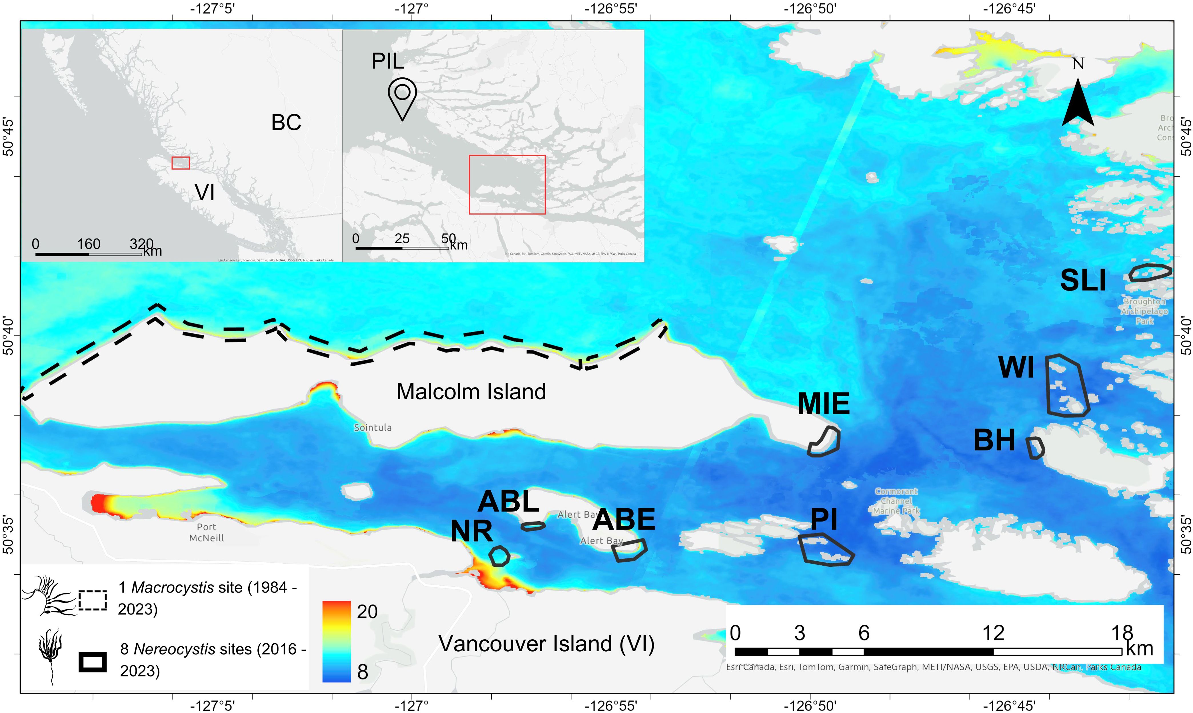
Figure 1. The main map shows the study area (the dynamic subregion of the Broughton Archipelago), with the Macrocystis site on the north shore of Malcolm Island marked in a dashed black outline and the eight Nereocystis sites marked in solid black outlines. The Nereocystis sites include kelp beds at Nimpkish River (NR), Alert Bay Lighthouse (ABL), Alert Bay East (ABE), Pearse Islands (PI), Bold Head (BH), Wedge Island (WI), and South Leading Islet (SLI). The background of the main map is the mean Landsat-derived SST from the summers (July and August) of 2016 to 2023. The left inset map shows the location of the study area at a provincial scale relative to Vancouver Island (VI) and mainland BC (BC). The right inset map shows the study area (marked by the red rectangle) situated within the Queen Charlotte Strait region, relative to the location of the Pine Island Lighthouse (PIL), from which the regional SST and MHW metrics were derived (see 2.2.1). Macrocystis and Nereocystis graphics were obtained from phylopic.org, with the former created by Harold N Eyster (CC BY 3.0, Attribution 3.0 Unported), and the latter created by Guillaume Dera (CC0 1.0 Universal Public Domain Dedication license.)

Local community members, including First Nations, have revealed that, generally, the kelp forests have declined in density and coverage in their territories (Broughton Aquaculture Transition Initiative (BATI), unpublished, 2021; Salmon Coast Field Station (SCFS), unpublished, 2023). Community members have also reported specific locations of kelp change in the region, including an increase around Malcolm Island, and decreases at an offshore kelp bed at the mouth of the Nimpkish River (“NR”), at a nearshore kelp bed off the shore of the Alert Bay Lighthouse (“ABL”), and along the salmon migration routes in the fjords near now-decommissioned open-net salmon farms (SCFS, 2023; Mountain, pers comm, 2023).

One Macrocystis site and eight smaller Nereocystis sites were selected to represent the temporal dynamics of kelp beds of different species and sizes exposed to different environmental conditions. The Macrocystis site encompasses the entire north shore of Malcolm Island (spanning 11.6 km²), and the eight smaller Nereocystis sites (ranging from 0.03-1.45 km² per site) represent the portion of the eastern shore of Malcolm Island with high kelp abundance and the smaller islands east of Malcolm Island (Figure 1). Only one Macrocystis site was selected as this was the only area within the Broughton Archipelago where Macrocystis was present. The bottom substrate type at the Macrocystis site was primarily mixed rocky and sandy substrate, with kelp growing on the rocky areas (Haggarty et al., 2020; Man et al., in prep). The smaller site approach was chosen for the Nereocystis sites rather than mapping all of their coastlines due to the geomorphological complexity of the area, which imposed a challenge for the satellite remote sensing of kelp because of the increased land adjacency effects (Cavanaugh et al., 2021). The Nereocystis sites included the offshore kelp beds at the mouth of the Nimpkish River (NR), the nearshore kelp beds off the shore of the Alert Bay Lighthouse (ABL), the eastern coastline of Alert Bay (ABE), the eastern tip of Malcolm Island (MIE), Pearse Islands (PI), Bold Head (BH), Wedge Island (WI), and South Leading Islet (SLI) (Figure 1). PI, BH, and WI had primarily shallow (<20 m depth) rocky bottom substrate, surrounded by deeper (>20 m) areas where kelp cannot grow (Haggarty et al., 2020). ABL, ABE, and MIE had mixed rocky and sandy bottom substrates, and NR and SLI had mixed rocky and sandy bottom substrates surrounded by pure sandy substrates which cannot support kelp growth (Haggarty et al., 2020).

The locations of the Macrocystis and Nereocystis sites were selected opportunistically during a field visit and based on their importance to the Mamalilikulla First Nation, ‘Na̱mg̱is First Nation, and Kwikwasut’inuxw/Haxwa’mis First Nation. These three Nations formed the Broughton Aquaculture Transition Initiative (BATI), a coalition that emphasized the need to continue monitoring and protecting the Archipelago’s kelp forests due to their importance as nearshore salmon habitat (BATI, unpublished, 2021). The Macrocystis and the Nereocystis sites experience slightly different environmental and topographical conditions from each other, with the Macrocystis site having flatter slopes and lower tidal current speeds than the Nereocystis sites (Davies et al., 2018; Foreman et al., 2009).

2.2 Data compilation and processing

The following data were compiled: (1) local, regional, and global-scale environmental conditions, (2) Landsat-derived canopy kelp area (1984 to 2023) at the Macrocystis site, and (3) Planetscope-derived kelp area (2016 to 2023) at the Nereocystis sites (both “kelp area” hereafter) (Figure 2). In addition, very high-resolution Worldview-2 and GeoEye-1 imagery was used to validate kelp classifications derived from Landsat and Planetscope imagery (Figure 2). The environmental variables were used to define climate periods (years with similar environmental conditions) (Figure 2). Objective 1 (identify the temporal responses of Macrocystis pyrifera and Nereocystis luetkeana, respectively, to changes in temperature and climatic oscillations) was achieved by analyzing both long-term and short-term kelp time series alongside environmental changes at local, regional, and global scales (Figure 2). Objective 2 (identifying spatial patterns of kelp persistence) was achieved by spatially combining yearly kelp areas (Figure 2).

Figure 2

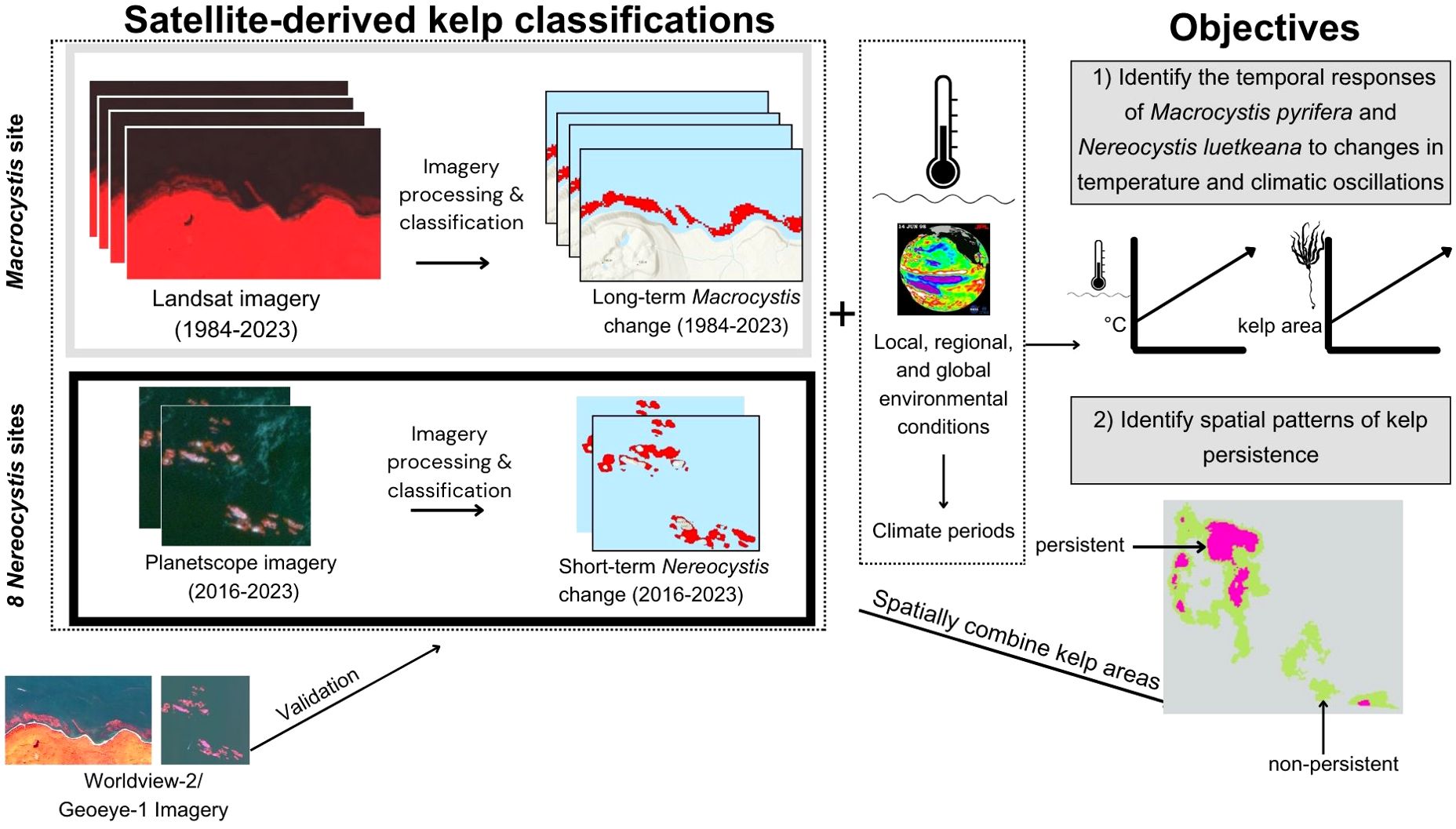
Figure 2. A flow chart representing the data compilation and processing, as well as the spatial and temporal dimensions of the study, and how satellite-derived kelp classifications and environmental data are combined to achieve the objectives of the study.

2.2.1 Environmental conditions

The environmental conditions from the past four decades (1984 to 2023) were compiled to evaluate their roles as drivers of kelp area change. Environmental data was acquired to represent three different spatial scales: 1) Local: Summer climatologies compiled from temporally discontinuous Landsat-derived SST from the Macrocystis and Nereocystis sites; 2) Regional: spring, and summer climatologies derived from temporally continuous (daily) in-situ SST measurements collected at Pine Island Lighthouse about 57 km north of the study area (Figure 1), representative of the Queen Charlotte Strait region; and 3) Global: annual ONI and PDO indices representing the climatic conditions of the broader Northeast Pacific Ocean.

Local SST

We characterized local SST changes in the study area by deriving mean summer (July-August) SST climatologies from the thermal infrared band of Landsat 5, 7, 8, and 9 imagery (“local SST” hereafter, spatial resolution: 30 m) for each year; note that this dataset was temporally discontinuous due to low availability of imagery related to frequent high cloud cover. Furthermore, only summer SST was considered for the local-level dataset due to the even more frequent high cloud cover present during spring in the Broughton Archipelago. To create the SST climatologies, we first compiled all cloud-free Landsat images captured during the summer months from 1984 to 2023, excluding years with only one cloud-free image to prevent skewing the summer mean with short-term extremes. As a result, only 13 years of mean local SST data were analyzed out of the total 40-year period for the Macrocystis site (Table 1). For each of the 13 years, mean local SST was calculated using zonal statistics in a polygon spanning the entirety of the Macrocystis site (Figure 1), buffered 300 m away from the shoreline. This reduced the interference of land temperature on the water pixels, producing accurate nearshore SST data (Wachmann et al., 2024). Mean local Landsat SST data for the Nereocystis sites were available for 26 out of the 39 years analyzed (Table 1). For each of these 26 years, local SST was calculated using zonal statistics in a 200-m radius buffer 300 m from any land (Wachmann et al., 2024). These annual mean summer SST measurements were then compiled into site-specific climatologies. Note that although local SST measurements for the Nereocystis sites were acquired between 1984 and 2023, their kelp time series only ranged from 2016 to 2023 due to the limited availability of Planetscope imagery.

Table 1

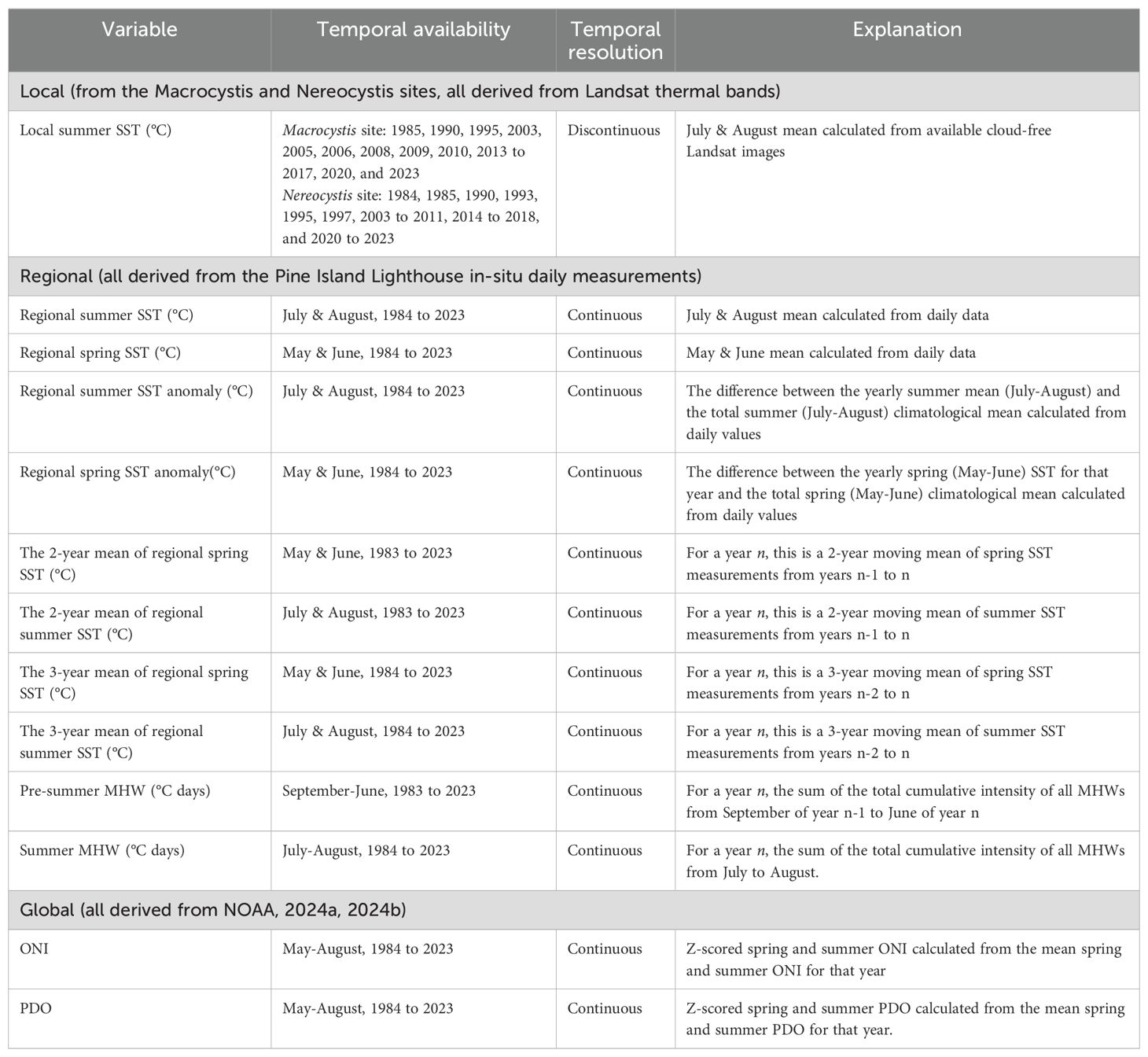
Table 1. The environmental variables at local, regional, and global scales.

Regional SST and MHWs

We characterized the regional SST based on daily in-situ SST measurements collected at Pine Island Lighthouse (“regional SST” hereafter), compiled from 1982 to 2023 (Fisheries & Oceans Canada, 2024⁷) (Figure 1). Pine Island Lighthouse is 57 km away from Malcolm Island, thus representing the general environmental conditions of the Queen Charlotte Strait region rather than the local conditions at the sites. However, its high temporal resolution allowed us to calculate MHW frequencies and magnitudes (Hobday et al., 2016, 2018).

The following metrics were calculated from the daily regional SST measurements: (i) spring (May-June), and summer (July-August) SST climatologies, (ii) mean yearly spring and summer SST anomalies, and (iii) two- and three-year mean climatologies of regional spring and summer SST. Spring and summer SST metrics represented the conditions during stages of high kelp growth and peak kelp biomass, respectively (Springer et al., 2010). Winter SST metrics, which would represent the environmental conditions present during the kelp gametophyte stages (Springer et al., 2010), were not included as there were a few winter months with no SST data collected (December 2018-January 2019, December 2019 to January 2020, and December 2020 to January 2021), compromising the continuity of the data. The two- and three-year SST means were computed for each season to evaluate the potential lagged effects of temperature changes on kelp (Pfister et al., 2018) (Table 1).

Beyond the SST metrics above, MHWs were identified from the regional daily SST measurements, with an MHW defined as when the maximum observed day temperature surpasses the day’s seasonal climatology and 90th percentile temperature threshold for more than five days, sensu Hobday et al. (2016). Following Hobday et al. (2016, 2018), we calculated four MHW categories (I - IV), corresponding to multiples of the seasonal difference between the climatological mean and the climatological 90th percentile. A Category I MHW surpasses the climatological 90th percentile once, and a Category II MHW twice, etc. Multiples of this difference vary by location and time of year; thus the category may not directly correspond to the maximum intensity. For example, a MHW on December 2, 2016, of maximum intensity 2.0°C, was classified as Category II because this event surpassed the climatological 90th percentile of this season twice, yet another MHW on September 24, 2019, of maximum intensity 2.5°C was only classified as Category I because this event surpassed the climatological 90th percentile of that season only once. After identifying the MHWs, the cumulative intensity of each MHW was calculated as the MHW’s temperature anomaly (°C) multiplied by the number of heatwave days. For each year n, the following metrics were noted: (i) total pre-summer MHW cumulative intensity, which is the cumulative intensity of all MHWs that occurred from September 1st of year n-1 to June 30th of year n, and (ii) total summer MHW cumulative intensity, which is the combined cumulative intensity of all MHWs between July and August of year n. The total pre-summer MHW cumulative intensity would represent the MHWs occurring in the fall and winter of year n-1, and in the spring of year n, which may affect the kelp spores and gametophytes that will eventually reach canopy height as sporophytes in year n (Springer et al., 2010), thus affecting the kelp area detected in year n. Although there were data gaps in the SST during the winter months from 2018 to 2020 (December 2018 - January 2019, December 2019 - January 2020, and November 2020 - Jan 2021), we determined that it was still suitable to use the pre-summer MHW metrics because some of these months were still represented, from September of year n-1 to June of year n. Regardless, this limitation should be kept in mind when interpreting the results for 2018-2020, where pre-summer MHW cumulative intensity may be underestimated.

Global: climatic oscillations

The global environmental conditions were characterized by the mean yearly ONI and PDO (NOAA, 2024a⁸, 2024b⁹). Mean yearly ONI and PDO were calculated from spring and summer (May to August) values and were then rescaled using Z-scores to identify when each index was above or below their 40-year climatological mean, following the methods of Mora-Soto et al. (2024a). This resulted in an ONI and PDO Z-score for each year (Table 1), with positive values indicating warmer years with less optimal conditions for kelp (Mora-Soto et al., 2024a)

2.2.2 Mapping canopy kelp area

Kelp area was quantified by classifying satellite imagery from 1984 to 2023. Higher-resolution satellite imagery was selected to map the floating kelp area in the Nereocystis sites than the Macrocystis sites, as higher-resolution imagery is more appropriate for mapping the fringing Nereocystis beds typical of this region (Cavanaugh et al., 2021; Gendall et al., 2023). Landsat imagery (spatial resolution: 30 m, 1984 to 2023) was selected to map the large kelp beds at the Macrocystis site, creating a longer time series. Planetscope imagery (spatial resolution: 3 m, 2016 to 2023) was used to represent kelp changes at the smaller Nereocystis sites after the Blob (Bond et al., 2015). Then, very-high-resolution Worldview-2 and GeoEye-1 imagery (spatial resolution: 0.46 and 1.84 m, respectively) obtained from 2017 and 2023 were used to validate the satellite-derived kelp area classifications.

Long-term Macrocystis time series

For the Macrocystis site, the kelp area was derived from Landsat imagery using two different classification approaches: Multiple Endmember Spectral Mixture Analysis (MESMA) (Cavanaugh et al., 2011; Bell et al., 2020) and Object-Based Image Analysis (OBIA) (e.g. Gendall et al., 2023; Mora Soto et al., 2024a). The mixture of approaches was used due to the availability of a pre-existing dataset from 1984 to 2020 (Reshitnyk, unpublished data, 2024) classified using MESMA. Additional classifications of kelp area using OBIA allowed us to expand the time series to include 2021 to 2023. For the 1984-2020 Landsat dataset, atmospherically corrected surface reflectance products (Landsat Collection 1 Level-2 reflectance data) were downloaded from the United States Geological Survey Earth Explorer website¹⁰ for the sites for Landsat sensors TM, ETM+, and OLI for each year. To mask out intertidal areas, a land mask was derived for the region using a single Landsat scene collection at a 0.2 m tide (Mean Lower Low Water) to remove all land and intertidal pixels (mask creation details in Supplementary material S1). Classification of the kelp area followed methods described by Bell et al., 2020. Following cloud and land masking, for each scene, a binary classification decision tree was used to classify each pixel into one of four classes: seawater, cloud, land, and kelp. A Multiple Endmember Spectral Mixture Analysis (MESMA) (Bell et al., 2020; Roberts et al., 1998) was used to determine the kelp fraction contained in each kelp pixel. We converted the fractional cover dataset to a binary time series based on a fractional kelp cover threshold of 13% (Houskeeper et al., 2022: Cavanaugh et al., 2011). The final dataset represents the maximum kelp area for a given year. 1992 was excluded from this analysis as there was no available cloud-free imagery for the study area.

For the 2021-2023 Landsat dataset, we used one yearly cloud-free Landsat image acquired during low tide between spring and summer, thus representing the kelp area captured at peak biomass (Springer et al., 2010). For each image, the land was masked out, and a Normalized Difference Vegetation Index (NDVI) and linear enhancements were applied to increase the spectral separability between kelp and water (following the protocols in Gendall et al. (2023). Each image was classified using an OBIA approach (OBIA classification methods in Supplementary material S2). For the entire time series (1984 to 2023), the kelp area was normalized as a percentage of the maximum kelp area, i.e. aggregated area of all kelp detected for the entire time series.

Short-term Nereocystis time series

Planetscope imagery was used to derive kelp areas for the short-term time series (2016 to 2023) covering the eight Nereocystis sites (Table 2). One cloud-free summer image acquired at a tidal height less than 2.50 m above the chart datum was used to derive each year’s kelp area. The processing and classification of the short-term time series followed the methods delineated in Gendall et al. (2023). Imagery from 2016 required atmospheric correction as only top-of-atmosphere reflectance products were available. Atmospheric correction was performed using a Rayleigh correction, with dark targets selected using the darkest pixel histogram adjustment method described in Hadjimitsis et al. (2004). Atmospheric correction was not conducted on imagery from 2017 to 2023, as surface reflectance products were available. In terms of geometry, georeferencing using a single-order polynomial transformation against the ArcGIS base map was conducted if an image was misaligned relative to the base map. Next, areas where kelp cannot grow (i.e. land, deep water (>20 m), and sandy and mud substrate) were masked from imagery to avoid false positives in kelp area classifications following the methods outlined in Gendall et al. (2023). The land mask was manually delineated based on the lowest tide Planetscope image (tidal height: 0.716 m) in this kelp time series, acquired on August 4, 2023; the sandy and mud substrate mask was created using the BC bottom patch model (Haggarty et al., 2020); and the deep water mask (depths >20.0 m) was created using a coastal digital elevation model for Pacific Canadian waters (Davies et al., 2018). Following the masking step, a Near-Infrared/Green (NIR/G) band ratio and linear enhancements were applied to the imagery before classification (Gendall et al., 2023). The images were subsequently classified using the aforementioned OBIA methods (see details in the classification methods in Appendix S2), resulting in yearly kelp area products from 2016 to 2023 for each Nereocystis site. Finally, yearly kelp areas were normalized into percent kelp area.

Table 2

Table 2. Table detailing imagery used for the long-term and short-term time series, as well as imagery validation.

Methods comparison and validation of kelp area products

We ensured that the MESMA-based yearly kelp aggregate area classification method (as used in 1984 to 2020 Macrocystis site classifications) and OBIA-based non-aggregate kelp area classification method (as used in 2021 to 2023 Macrocystis site classifications and 2016 to 2023 Nereocystis site classifications) created comparable results by conducting a sensitivity analysis. Two Landsat summer images, from 1986 and 2015, covering part of the Macrocystis site already classified using MESMA, were additionally classified using OBIA. The percent kelp area derived from the OBIA classification was within a 1% difference from that of the MESMA classification; thus, the two classification methods were deemed comparable.

Moreover, we confirmed that there were no confounding effects of tidal height on the percent kelp area by fitting a linear mixed model for the short-term time series (tidal height range: 0.716-2.500 m), with percent kelp area as the dependent variable, tidal height as a fixed effect, and site as a random effect (R package “lme4”, Bates et al., 2015). This analysis confirmed that the percent kelp area was not significantly affected by tidal height (p=0.320) and, therefore, suitable for use in subsequent data analysis. This test was not conducted for the long-term time series as the kelp area for each year was derived from multiple images of various tidal heights, minimizing the tidal height-induced variability associated with this dataset.

The satellite-derived kelp area products were validated by comparing the spatial overlap between the kelp classifications and very high-resolution satellite images (spatial resolution: 0.460-1.84 m). The very high-resolution satellite images provided more accurate representations of the kelp beds due to the reduced pixel mixing between kelp and water (Cavanaugh et al., 2021; Gendall et al., 2023). As the validation of all the yearly kelp classifications was challenging due to the lack of historical in-situ data and very high-resolution imagery, we selected one year to validate the kelp classification approach of each of the time series and assumed this validation would be representative of the other years. For the long-term Macrocystis time series, a Worldview-2 image (spatial resolution: 1.84 m, acquired on August 1, 2017), was used to validate the Landsat-based classification of the Macrocystis site kelp beds from 2017. For the short-term Nereocystis time series, we validated the 2023 Planetscope-derived classifications of six Nereocystis sites’ kelp beds by using a pan-sharpened Worldview-2 image (spatial resolution: 0.46 m, acquired on August 4, 2023) and a pan-sharpened GeoEye-1 image (spatial resolution: 0.46 m, acquired on August 6, 2023) (Table 2). Overall accuracy of 89.7% and 89.1% were found for the long-term and the short-term time series, respectively (Details on validation methods and results in Supplementary Material S3, Supplementary Table S1).

2.3 Data analysis

2.3.1 Identifying environmental trends at different spatial scales and climate periods

The Modified Mann-Kendall test (Hamed and Rao, 1998, R package: rtrend), a non-parametric test for monotonic trends adjusted for serial autocorrelation, was used to investigate significant temporal trends of local summer SST climatologies, regional spring and summer SST climatologies, and MHWs. Here, a significant and positive Z-statistic would indicate an increasing trend, a significant and negative Z-statistic would indicate a decreasing trend, and a non-significant test result would indicate no significant temporal trends. We did not test for trends in PDO and ONI as these climatic oscillations are inherently cyclical (Norel et al., 2021).

The time series of environmental variables were statistically organized into climate periods to define kelp area changes between these periods. This is because kelp can generally show lagged fluctuations for one to two years in response to environmental conditions due to the potential multi-year impacts of environmental changes (Pfister et al., 2018; Mora-Soto et al., 2024a). The climate periods were identified by defining changepoints, i.e., points in the time series where abrupt changes in temporal trends occur (Zhao et al., 2019), in the regional spring and summer SST. These datasets were selected to define the transitions between climate periods because of the in-situ nature and the continuity of the time series (Table 1); the local satellite-derived SST data was not fit for this analysis due to its temporally discontinuous nature (see section 2.2.1). The changepoint analysis was conducted using the Bayesian Estimator of Abrupt change, Seasonal change, and Trend (BEAST) algorithm, an ensemble algorithm that leverages time series decomposition models using Bayesian model averaging (Zhao et al., 2019, R package: rBeast). We further conducted Kruskal-Wallis tests to define significant differences in each environmental variable (Table 1) between climate periods, and Dunn’s tests with the Benjamani-Hochberg adjustment for multiple testing were used for post hoc comparisons (Kruskal and Wallis, 1952; Dunn, 1964; Benjamini & Hochberg, 1995).

2.3.2 Long-term (1984 to 2023) and short-term (2016 to 2023) kelp response to environmental changes

The modified Mann-Kendall test (Hamed and Rao, 1998) was used to define both long-term (1984 to 2023) and short-term (2016 to 2023) temporal trends in the kelp area at each site. Here, a significant and positive Mann Kendall’s Z-statistic would indicate increasing kelp area, a significant and negative Z-statistic would indicate decreasing kelp area, and a non-significant test result would indicate no significant temporal trends. An increase or no significant change in the kelp area would indicate temporal persistence.

In addition, for the long-term Macrocystis time series, the Kruskal-Wallis test (Kruskal and Wallis, 1952) was conducted to identify potential differences in kelp area between the climate periods. Dunn’s test was used for post hoc comparisons, with the Benjamini-Hochberg correction for multiple testing (Dunn, 1964; Benjamini & Hochberg, 1995). Furthermore, linear models with different combinations of regional and global environmental variables were tested to define the most significant environmental variables affecting changes in the kelp area. The tested variables (predictors) included yearly, two-year, and three-year average climatologies of spring and summer SST/SST anomalies, pre-summer and summer MHWs, PDO, and ONI. The Landsat-derived local SST climatologies were not used as predictors in this linear model due to the lack of data for several years of the time series. All the predictor variables were tested for collinearity using Kendall’s correlation test and visual data exploration (Kendall, 1948). The Akaike Information Criteria (AIC) (Akaike, 1974) was used to determine the most suitable combination of predictors from the non-autocorrelated variables. The assumptions of the linear model were visually evaluated with histograms of the model residuals, residuals’ quantile-quantile plots, plots of the fitted values vs residuals, and statistically evaluated for the normality assumption using Shapiro-Wilk tests (Shapiro and Wilk, 1965). A plot of the residuals vs the observed site numbers was used to identify patterns in the order of the data, which tests for the assumption of the independence of observations, whereas a plot of the models’ fitted vs residuals values was used to test for the linearity and constant variance assumptions. All visualizations were consistent with the assumptions required by the model, and the result of the Shapiro-Wilk tests confirmed that the model residuals were normal.

A similar comparison of kelp area change across climate periods and linear model analysis of the effect of environmental conditions were not conducted for the Nereocystis sites due to the reduced time series. However, a descriptive characterization of the observed kelp percent area change and the local environmental conditions during and after the end of the Blob (2016 to 2023) was conducted. These included noting down the mean local summer SST at each site, identifying the hottest and coolest sites, as well as years of kelp loss.

2.3.3 Spatial patterns of kelp persistence

Persistent kelp areas within the maximum kelp area were defined as areas (m²) where kelp was present for more than 50% of the time-series length (>19 years of presence for the long-term Macrocystis time series; >4 years for the short-term Nereocystis time series). Our definition of a persistent area was adapted from the “refugia” definition of Cavanaugh et al. (2023), who identified as refugia areas of kelp that occurred in 50% of the years in a Planetscope-derived time series (2016 to 2021 in their case). We simply defined these as “persistent” areas rather than “refugia”, as the study area did not experience environmental conditions detrimental to kelps as the term “refugia” would imply (see results). We identified the spatial distribution of kelp persistence at each site using the ‘Count overlapping features’ tool in ArcGIS Pro 3.0 (ESRI, Redlands, United States), which indicated where and how many times the yearly kelp areas overlap, using the ‘Count overlapping features’ tool in ArcGIS Pro 3.0 (ESRI, Redlands, United States). Finally, the percent of the persistent kelp area $\left(\frac{persistent kelp area}{maximum kelp area}\right)$ was calculated for each site.

3 Results

3.1 Environmental conditions and their differences among climate periods at local, regional, and global scales

At the regional level, the mean spring SST ranged from 8.4°C to 11.1°C, and mean summer SST ranged from 9.6°C to 12.6°C (Figure 3, SST anomalies in Supplementary Figure S1), with no temporal trends in either regional spring or summer SST (modified Mann-Kendall’s test: spring: Z-statistic = 0.187, p=0.0911; summer: Z-statistic = 0.195, p=0.0785; Table 3). Based on the mean summer and spring regional SST, the changepoints analysis (Supplementary Table S2) indicated three climate periods: Period 1 represents generally warmer ocean temperatures from 1984 to 1998, Period 2 represents cooler temperatures from 1999 to 2013, and Period 3 represents the highest temperatures of the time series from 2014 to 2023 (Figure 3). Accordingly, mean spring and summer regional SST were different across all periods (Figure 3, Table 3). For both spring and summer, Period 1 (spring SST: 9.8 ± 0.41°C, summer SST: 10.7 ± 0.31°C) had significantly warmer SST than Period 2 (spring SST: 9.2 ± 0.47°C, summer SST: 10.1 ± 0.41°C, Figure 3, Table 3). Furthermore, Period 3 (spring SST: 10.5 ± 0.37°C, summer SST: 11.6 ± 0.5°C, summer SST anomaly: 0.9 ± 0.53°C) had significantly warmer SST than both Periods 1 and 2 (Figure 3, Table 3).

Figure 3

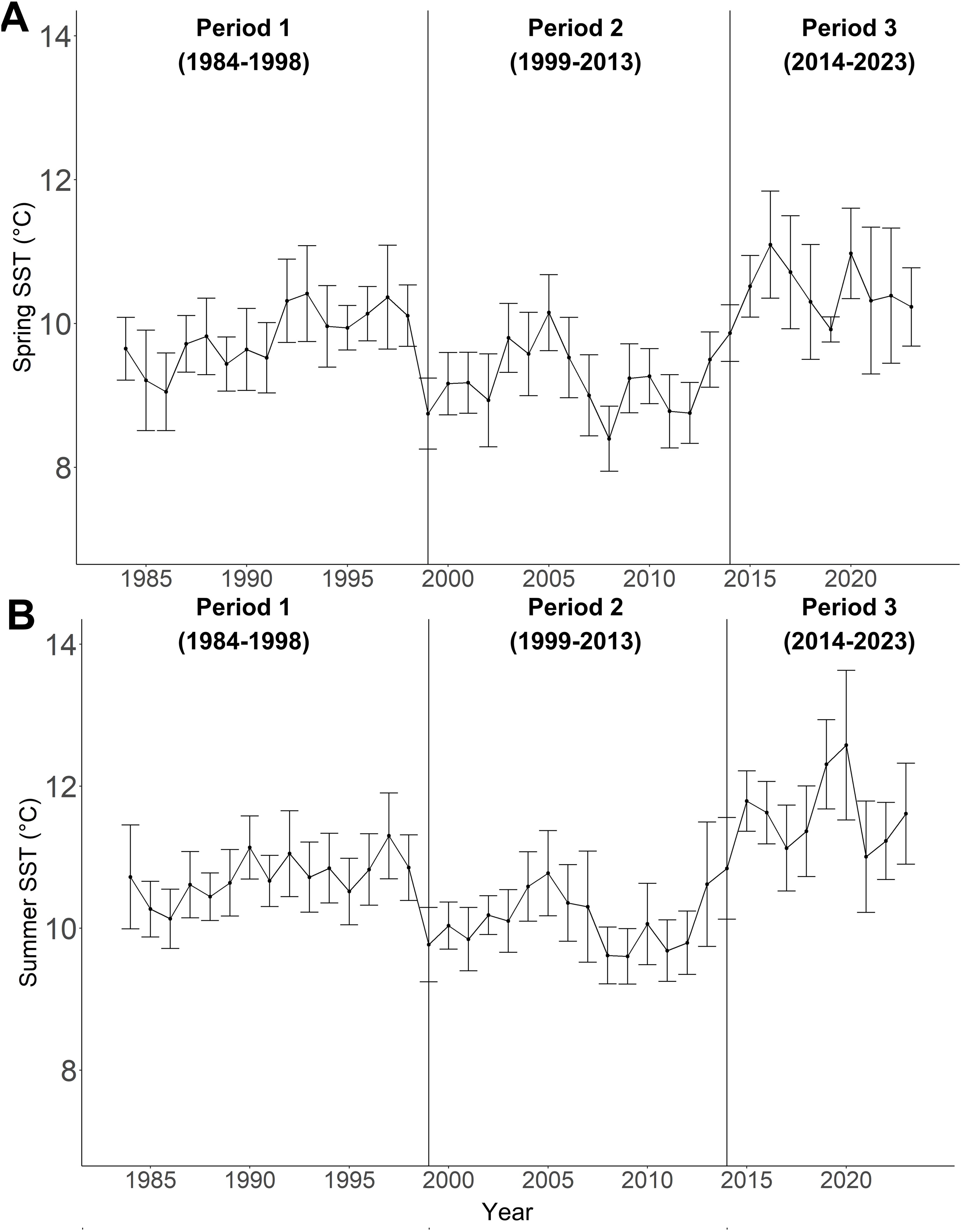
Figure 3. (A) Mean regional spring SST, and (B) mean regional summer SST from 1984 to 2023. All data was derived from the Pine Island Lighthouse daily SST climatology (1984 to 2023), with error bars representing the standard deviations. The vertical black lines depict the transitions between the climate periods.

Table 3

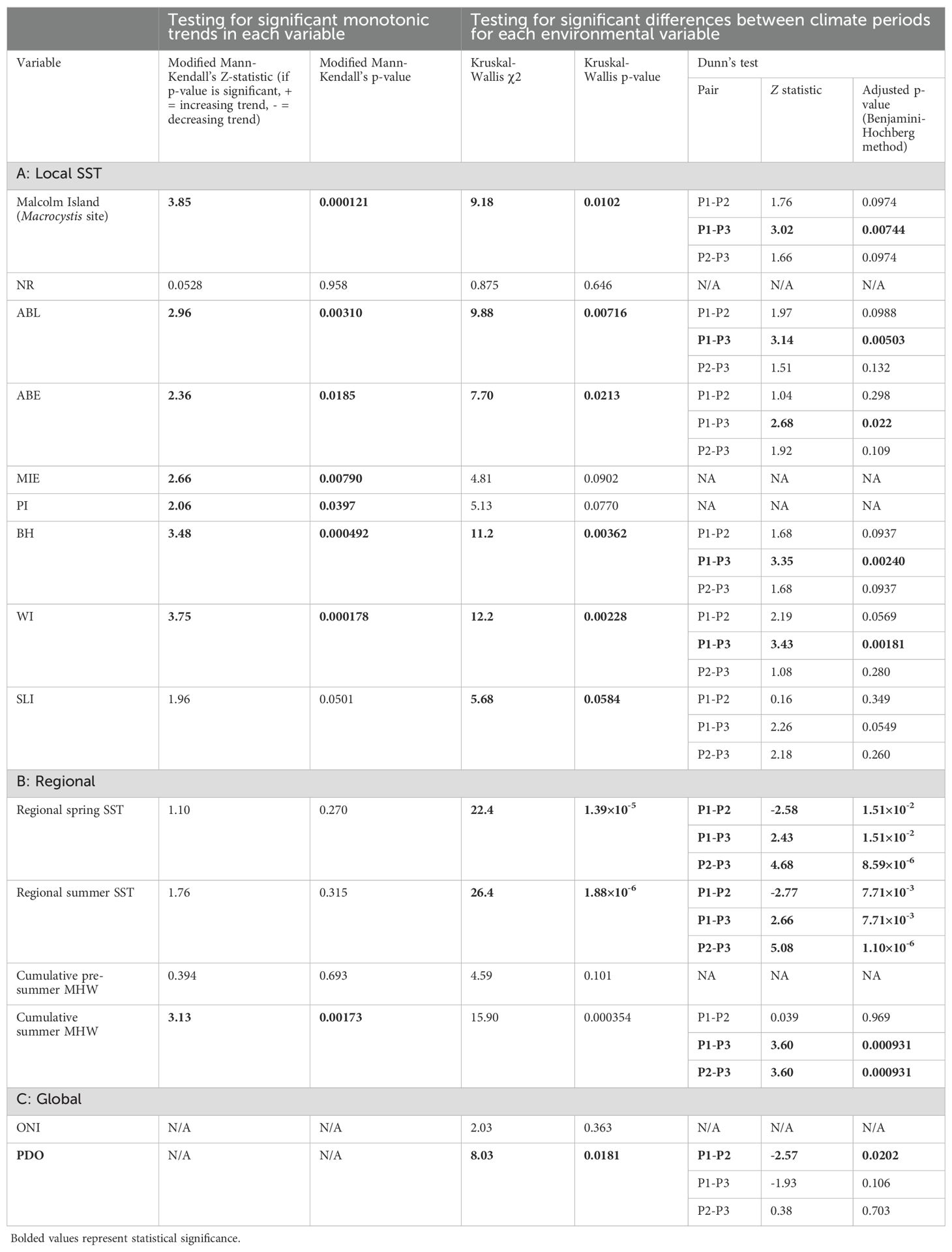
Table 3. Mann-Kendall’s test results testing for significant increases, decreases, or lack thereof in environmental variables from 1984 to 2023, with cells colored in grey, and Kruskal-Wallis and Dunn’s test results representing environmental differences between climate periods with cells colored in white (P1 = Period 1, P2 = Period 2, P3 = Period 3) at A) local, B) regional, and C) global scales.

At the local scale, the Landsat-derived SST showed some variability, with the Macrocystis site presenting warmer SST (11.5 ± 0.96°C) (climatological summer mean ± standard deviation) than the Nereocystis sites (10.1 ± 1.05°C). On average, the hottest Nereocystis sites were ABL, ABE, and SLI (~10.3°C), and the coolest Nereocystis site was BH (9.4 ± 0.72°C) (Figure 4A, Supplementary Table S3). Across the three identified climate periods, the mean local SST significantly increased for the Macrocystis site and six Nereocystis sites (ABL, ABE, MIE, BH, WI, PI) (Figure 4A, Table 3A), with ~1.4°C (Table 3A) higher SST in Period 3 (Macrocystis site: 12.5 ± 0.42°C, Nereocystis sites: 10.6 ± 0.71°C) than in Period 1 (Macrocystis site: 10.3 ± 0.20°C, Nereocystis sites: 9.2 ± 0.54°C). However, neither Periods 1 nor 3 had significant differences with Period 2 regarding the mean local SST (Figure 4B, Table 3A). For the other two Nereocystis sites (NR, SLI), local SST measurements were not significantly different among the periods (Figure 4B, Table 3A), although local SST peaked in 2004 in sites NR and SLI, reaching mean summer temperatures of 14.2 ± 1.50°C and 12.0 ± 0.31°C. respectively.

Figure 4

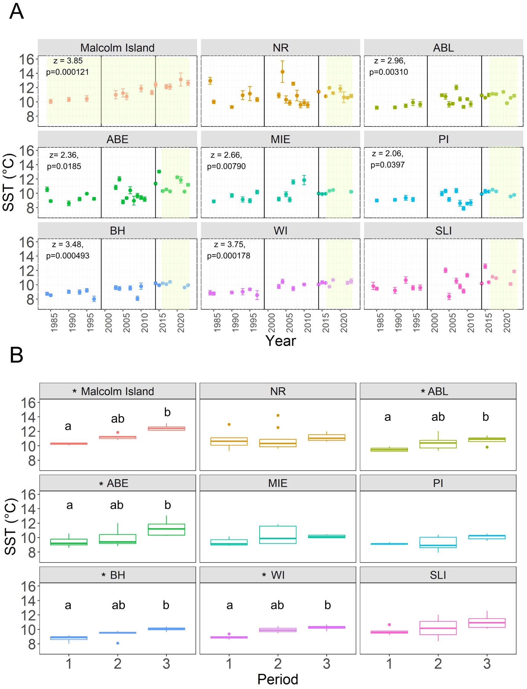
Figure 4. (A) Scatterplot showing the mean local summer SST for the Macrocystis site (“Malcolm Island”) and each Nereocystis site (as denoted by the abbreviated site names) from 1984 to 2023, with the error bars around each point representing the standard deviation for each year. The vertical black lines in 1999 and 2014 represent the boundaries between climate periods. The modified Mann-Kendall’s Z-statistic and p-value are reported in the top left corner for sites with significant monotonic trends. The green shaded areas of each site’s panel represent the length of the kelp time series analyzed for each site. (B) The differences in mean local summer SST between each period. Sites with an asterisk (*) are sites with significant differences in local SST across periods. Different letters above each boxplot denote significant pairwise differences.

On the regional scale, 57 MHWs were identified between January 1983 and August 2023. Among these, 27 were in Category I, 23 in Category II, 6 in Category III, and 1 in Category IV (Figure 5A). The most intense (Category IV) MHW occurred on 30 July 2020, lasting six days and reaching a maximum temperature intensity of 15.4°C (a +4.7°C anomaly), with a total cumulative intensity (calculated as the mean temperature anomaly of the MHW multiplied by the number of heatwave days) of 18.2°C days. The most cumulatively intense MHW occurred at the beginning of 2016, starting on 20 January and lasting 98 days, resulting in a cumulative total of 146.0°C days, and reaching a maximum intensity of 10.8°C (a +2.2°C anomaly). Note that there were several winter months with no SST data available, namely December 2018 - January 2019, December 2019 - January 2020, and November 2020 - Jan 2021 (see section 2.2.1), thus the lack of MHWs detected during those periods may be attributed to this reason. Furthermore, the pre-summer cumulative MHW intensity may be underestimated as a result. The pre-summer MHW time series did not display any temporal trends, but the summer MHW time series exhibited a statistically significant increase (Table 3B). Pre-summer MHW cumulative intensity was not significantly different across periods. However, summer MHW cumulative intensity was different across Periods 1 and 3, and 2 and 3, with Period 3 representing the highest MHW intensity (Period 1: 1.2 ± 54.32°C days, Period 2: 1.7 ± 6.21°C days, Period 3: 26.4 ± 106.84°C days) (Supplementary Figure S2, Table 3B). Note that Period 3 had a high standard deviation for cumulative summer MHW intensity because most days did not have MHWs, but the MHWs that did occur had high cumulative intensity (°C days).

Figure 5

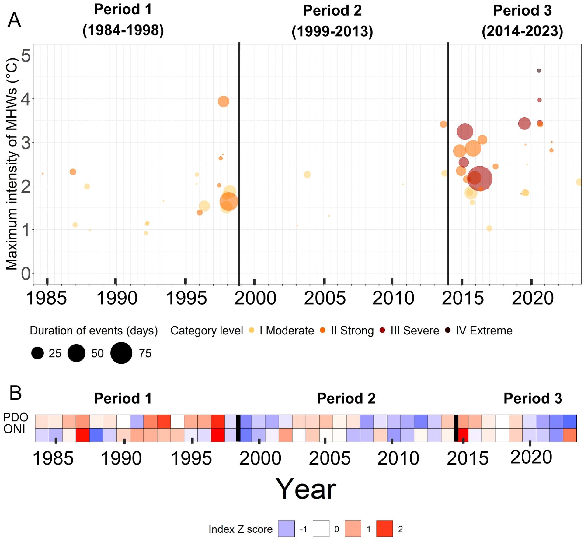
Figure 5. Regional and global conditions across the three climatic periods identified (Period 1, Period 2, and Period 3). For both panels, the black lines represent the transitions between climate periods. (A) MHWs and their associated duration and category level. The x-axis shows the date of each MHW’s maximum intensity peak, and the y-axis shows the maximum intensity of each MHW. The size of each dot corresponds to the duration of each MHW. The MHW category corresponds to the multiples of the seasonal difference between the climatological mean and the climatological 90th percentile. The color of each MHW corresponds to its category level, with a darker color representing a higher category. (B) Z-score of mean spring and summer Pacific Decadal Oscillation (PDO) and Oceanic Niño Index (ONI) from 1984 to 2023.

On the global scale, Period 1 (1984 to 1998) generally showed positive PDO (mean Z-score ± SD: 0.617± 0.855) and ONI (0.203 ± 1.13) values, reaching the highest PDO (2.09) and the second highest ONI (2.20) of the time series in 1997 (Figure 5B). Interestingly, the lowest ONI (-1.84) in the time series was also documented within Period 1 in 1988. Period 2 (1999 to 2023) displayed mostly negative PDO (-0.425 ± 0.817) and ONI (-0.292 ± 1.13), although a positive PDO and ONI were documented from 2002 to 2007. When comparing differences in oscillations between Periods 1 and 2, PDO was significantly more negative in Period 2 than in Period 1, whereas there were no significant differences in ONI (Figure 5B, Table 3C). Period 3 (2014 to 2023) started with positive ONI (0.180 ± 1.12) and PDO (-0.273 ± 1.09), with the highest ONI of the time series (2.21) documented in 2015. However, from 2020 onwards, both ONI and PDO shifted negative, with PDO reaching its lowest value of the time series (-1.91) in 2023, although ONI became positive again in 2023 (1.47). Ultimately, there were no significant differences in both ONI and PDO between Periods 1 and 3, and between Periods 2 and 3 (Table 3C).

3.2 Long-term (1984 to 2023) and short-term (2016 to 2023) kelp response to environmental changes

The maximum kelp area at the Macrocystis site (1984 to 2023) covered 4.84 million m². Percent kelp area ranged from 24.0% (absolute area: 1.15 million m²) to 71.0% (3.44 million m²), with a mean of 50.0% (2.46 million m²) of the maximum kelp area. Further, we found a statistically significant increase in kelp area (Mann Kendall’s τ=0.247, p=0.0300, Figure 6A) across all three climate periods. Among the climate periods, we observed statistically significant differences in kelp area between Periods 1 and 2 and between Periods 1 and 3, but not between Periods 2 and 3 (Figure 6A). Specifically, there was a slight increase in kelp area from 43.9 ± 9.34% in Period 1 to 53.8 ± 11.5% in Period 2, which remained high at 55.4 ± 10.4% in Period 3 (Figure 6B; Kruskal-Wallis χ2 = 7.56, p=0.0228; Dunn’s test: Period 1 vs Period 2: χ2 = 2.35, p=0.0380; Period 1 vs Period 3, χ2 = 2.35, p=0.0380, Period 2 vs Period 3, χ2 = 0.348, p=0.727). Considering the kelp time series in its entirety, without division between climate periods, the results of the linear model showed no effects of 1-, 2-, or 3-year averages of spring and summer SST, pre-summer and summer cumulative MHW intensities, PDO, or ONI on kelp area, regardless of the combination of predictor variables used (Supplementary Table S4).

Figure 6

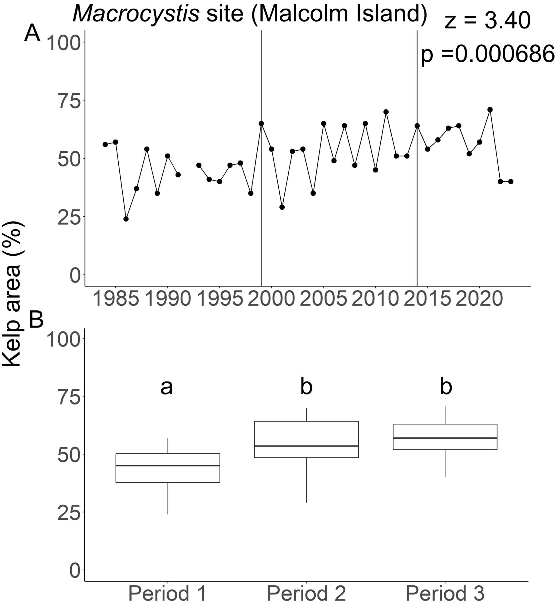
Figure 6. Kelp area changes in the Macrocystis site (Malcolm Island). (A) The temporal changes in the yearly kelp area from 1984 to 2023. Vertical lines in A) indicate the boundaries between periods. The Z-statistic represents the direction of monotonic change as determined by the modified Mann-Kendall’s test, with negative values representing negative trends and positive value representing positive trends. The p represents the p-value. There is no data available for 1992. (B) Boxplots showing the differences in the median kelp area and their associated interquartile ranges among climate periods. Identical letters above the boxes represent no significant differences in median kelp area between the pair of periods as determined by the Kruskal-Wallis test, whereas different letters above the boxes represent significant differences in median kelp area between the respective periods.

For the short-term time series, the maximum kelp areas across all Nereocystis sites ranged from 11,800 m² (BH) to 214,000 m² (MIE) (Figure 7). On a site level, mean percent kelp areas across all surveyed years ranged from 19.0 ± 30.2% (4,010 ± 6,360 m²) at ABL to 58.5 ± 13.3% at PI (111,000 ± 25,100 m²), with a total mean percent kelp area across all sites of 43.1 ± 19.3% (Figure 7) Most sites’ mean kelp areas exhibited parametric behavior, except ABL, which had a left-skewed pattern caused by kelp loss in the years 2018, 2019, 2022, and 2023 (Figure 7). The eight Nereocystis sites also displayed variable temporal trends in kelp areas from 2016 to 2023. Six Nereocystis sites displayed no temporal trends (ABL, MIE, PI, BH, WI, SLI), one displayed a significantly increasing trend (NR, modified Mann-Kendall’s Z-statistic = -4.26, p=0.000203), and one displayed a significantly increasing trend (ABE, modified Mann Kendall’s Z-statistic = 2.85, p=0.00443, Figure 7).

Figure 7

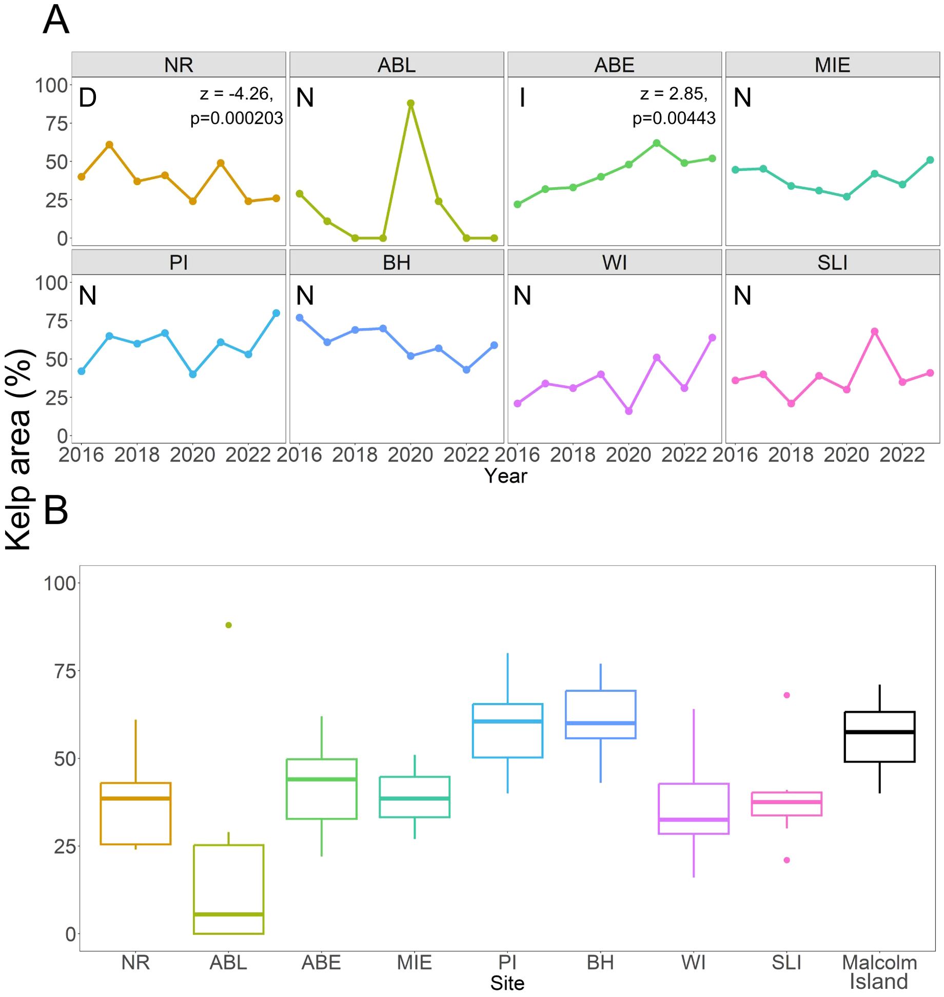
Figure 7. (A) Changes in percent kelp area in the 8 Nereocystis sites from 2016 to 2023. Sites with “N” under the site name are sites with no significant temporal trends, the site with “D” had a significantly decreasing trend, and the site with “I” had a significantly increasing trend, as per the modified Mann-Kendall test results. The significant test result is shown for the associated site. (B) Boxplot showing median kelp area and their associated interquartile ranges from 2016 to 2023 at each site. The mean percent kelp area for the Macrocystis site (“Malcolm Island”) from 2016 to 2023 is also included for reference, although it is not part of the short-term time series.

3.3 Spatial patterns of kelp persistence

The spatial analysis indicated that the Macrocystis site had 77.0% persistence, i.e., 77.0% of the maximum kelp area was present for more than 19 years out of the 38-year time series (Figure 8). The Macrocystis beds at the eastern part of the Macrocystis site were less spatially persistent than the western part (Figure 8). Five Nereocystis sites (NR, ABE, MIE, WI, SLI) had 20.6-33.8% persistence, i.e., area that was present for more than 4 years out of the 8-year time series (Figure 9). Sites PI and BH had larger proportions (53.1% and 53.6% respectively) of persistent kelp area, and ABL had no persistent kelp area (0.00% area). For both Macrocystis and Nereocystis sites, the persistent areas were mainly distributed in the center and inshore areas of each kelp bed (Figures 8-9).

Figure 8

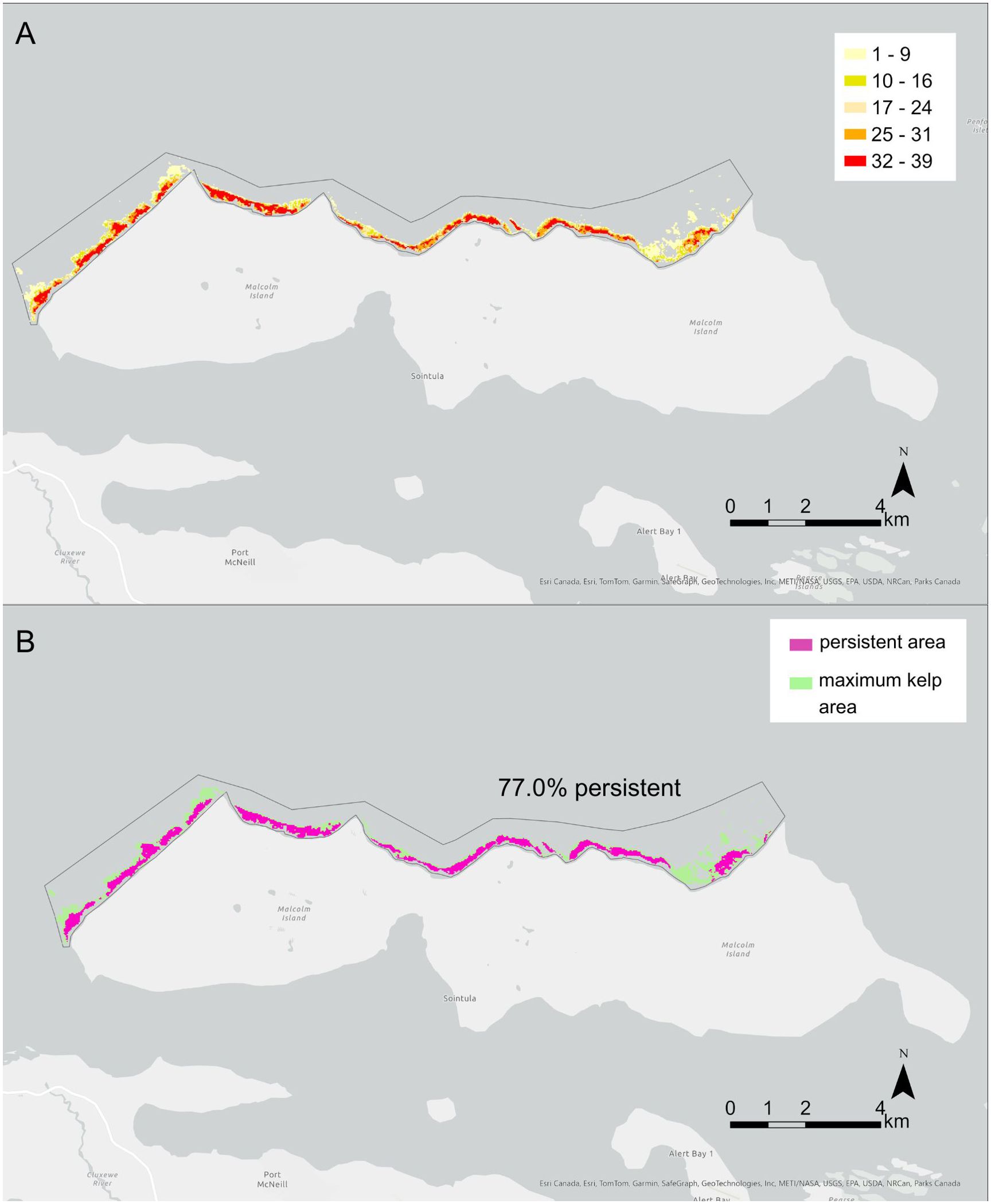
Figure 8. Maps showing the spatial patterns of kelp persistence at the Macrocystis site: the north shore of Malcolm Island. (A) shows the number of years of kelp presence out of the 39 years investigated, which was used to determine the areas of kelp persistence. The yellow-red scale indicates the number of years of kelp presence. (B) shows the persistent area in pink and the maximum kelp area in green. The total percentage area of the maximum kelp area that is persistent is indicated in (B) For both panels, the frame around the kelp beds shows the area considered for the analysis. Refer to Figure 1 for the location of the Macrocystis site.

Figure 9

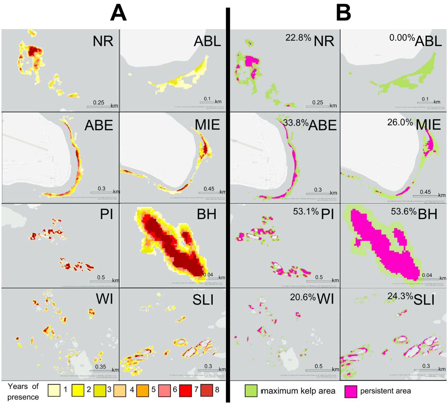
Figure 9. Maps showing the spatial patterns of kelp persistence at each Nereocystis site. (A) shows the number of years of kelp presence out of the eight years investigated, when higher resolution satellite images were available, which was used to determine the areas of kelp persistence. The yellow-red scale indicates the number of years of kelp presence. (B) shows the persistent area in pink and the maximum kelp area in green. The total percentage area of the maximum kelp area that is persistent is indicated in (B) Refer to Figure 1 for the location of each Nereocystis site.

4 Discussion

We found that kelp was both spatially and temporally persistent in the dynamic subregion of the Broughton Archipelago, with increases in the area occupied by Macrocystis. Specifically, we identified temporal trends in the kelp area and associated them with the changing environmental conditions using a long-term kelp change time series from 1984 to 2023 of the Macrocystis site and a short-term kelp change time series from 2016 to 2023 of the Nereocystis sites. We also identified spatial patterns of persistence by spatially combined kelp areas for each site.

4.1 Long-term (1984 to 2023) and short-term (2016 to 2023) kelp response to environmental changes

Overall, the kelp area in the Broughton Archipelago was mostly temporally persistent. Kelp percent area increased monotonically in the Macrocystis site from 1984 to 2023, specifically increasing by 9.90% in Period 2 and staying high throughout Period 3. The increase in kelp area at the Macrocystis site on the north shore of Malcolm Island corroborates reports from community members (SCFS, unpublished, 2023). This temporal increase indicated persistence in Macrocystis area from 1984 to 2023, which may be explained by the increase in local SST from ~10.0 to 13.0°C. This potentially represents a move towards more ideal environmental conditions for Macrocystis, which has an optimal thermal range from 12.0 to 17.0°C (Lüning and Neushul, 1978), although this range could vary among populations and life stages (e.g. spores, gametophytes, or sporophytes) (Muth et al., 2019; Hollarsmith et al., 2020; Le et al., 2022). For example, an increase from 9.5 to 12.9°C was experimentally associated with a ~5.00 μm increase in Macrocystis gametophyte germ-tube length (Le et al., 2022), and a 10.0 to 14.0°C increase to be associated with a ~2% increase in the relative growth rate of Macrocystis blades (Fernández et al., 2020). The local SST increases in the study area always remained below the upper thermal limits for Macrocystis, which lie around 18.0-25.0°C (Hay, 1990; Le et al., 2022; Ladah and Zertuche-González, 2007).

On the contrary, regional and global environmental conditions were not linked to significant changes in kelp area (based on the linear model results, Supplementary Table S4). This is likely as regional and global conditions occasionally diverged from the conditions kelps were facing locally in the nearshore environment (Brewer-Dalton et al., 2014; Lin and Bianucci, 2023). For example, the colder SST in Period 2 was only observed in the regional SST and inferred from the negative PDO, but not the local SST time series, which increased continuously throughout all three climate periods. Furthermore, occasional intense MHWs and higher local SST were observed during and after 2020, despite a shift to more negative ONI and PDO during the same time. A similar disparity was found between local SST and global climatic oscillations in other parts of BC. For instance, local SST continuously increased after 2020 in the Salish Sea, despite climatic oscillations transitioning to negative phases (e.g. Amos et al., 2015; Mora-Soto et al., 2024a), suggesting that the local SST increase in the Broughton Archipelago may be linked to local oceanographic conditions and variation in coastal geomorphology (Brewer-Dalton et al., 2014; Lin and Bianucci, 2023). Despite mismatches in environmental conditions of different scales during certain years of the time series, generally speaking, Period 3 had higher local and regional SST, a higher frequency and magnitude of MHWs, and more positive PDO and ONI. Similar conditions observed in the Strait of Georgia and Barkley Sound resulted in a subsequent decrease in kelp area (Mora-Soto et al., 2024a; Starko et al, 2022). However, in the dynamic subregion of the Broughton Archipelago, both local and regional measurements of SST remained within Macrocystis’ optimal thermal range during Period 3, and consequently, we did not observe decreases in the kelp area. This reinforces the observation that local temperature gradients can greatly influence kelp responses in the face of regional events such as MHWs (Starko et al., 2024b). It is unknown whether the climatic oscillations affected other environmental conditions not investigated in this study (e.g. nutrient availability) (Whitney, 2015; Bond et al., 2015), which may have impacted kelp physiology (Hollarsmith et al., 2022). Regardless, climatic oscillations did not directly relate to significant changes in the kelp area at the Macrocystis site.

Aside from environmental changes, there may be biotic conditions at play, such as a low abundance of sea urchins (Eisaguirre et al., 2020). Although not investigated in this study, Man et al. (in prep) found no sea urchins during a one-time sampling effort during the summer of 2023 at the Macrocystis site, suggesting that the absence or low abundance of sea urchins may have been conducive to kelp persistence at the Macrocystis site. Continuous time-series data about other environmental and biotic conditions could elucidate what specifically drove the increase in Macrocystis area in the study area.

Our observations of Macrocystis persistence in cooler waters corroborated patterns observed in cooler areas throughout the Northeast Pacific coast. For instance, centennial increases in the Macrocystis area were also observed in Southeast Alaska by Hollarsmith et al. (2024), which the authors attributed to various factors including temperature increases and the reintroduction of the sea otter, a keystone predator. Persistence in Macrocystis area was also observed in Cumshewa Inlet (Gendall et al., submitted), Ella Beach, BC (Mora-Soto et al., 2024a), and the outer coast of Washington (Pfister et al., 2018), where local summer SST increases (~10.0 to 14.0°C) over the past few decades were similar to those observed in the Broughton Archipelago and did not reach the upper thermal limits of Macrocystis. Similarly, these cooler, northern regions (BC and Washington) displayed Macrocystis persistence in response to the Blob of 2016. Conversely, the warmer southern regions (Central to Southern California, and Baja California Norte and Sur), which reached summer temperatures of ~17.0-24.0°C, experienced areal decreases to ~2-57% of their pre-Blob baseline (Mora-Soto et al., 2024b; Pfister et al., 2018; Cavanaugh et al., 2019; Bell et al., 2023).

Kelp persisted in most of the Nereocystis sites from 2016 to 2023, although some sites showed different trends in the kelp area. Specifically, ABL did not display a significant temporal trend, but exhibited kelp losses in four of the eight studied years, corroborating community anecdotes of kelp decrease in the area (SCFS, unpublished, 2023). Similarly, kelp also declined significantly at NR, confirming community reports of kelp decrease near Alder Bay and Green Island, which comprise the eastern areas of NR (Figure 9; SCFS, unpublished, 2023). An examination of Figure 9 revealed that the eastern areas of NR were indeed less spatially persistent. The observed increase in kelp area at ABE also reinforced local reports of a recent increase in kelp area after past decreases (SCFS, unpublished, 2023). Some of our results, however, contrasted with some other community reports of kelp trends: e.g. a kelp increase at MIE after urchin harvesting began in that area, although the start date of urchin harvesting was not reported (Mountain, pers comm, 2023). Such discrepancies between the local community members’ observations and our results may be linked to different study periods or time scales since they did not report the years where the changes in the kelp area were observed (SCFS, unpublished, 2023; Mountain, pers comm, 2023). Thus, it is possible that the changes identified by the local community were observed outside of the timeframe covered in this study between 2016 to 2023. Furthermore, short-term studies (<20 years) are less likely than long-term studies (>20 years) to capture patterns of kelp decrease due to kelp’s high interannual variability and environmental conditions’ multi-year or decadal dynamics (Wernberg et al., 2019). Therefore, it is also possible that our short-term time series was simply not long enough to detect the changes reported by local communities, or that Nereocystis’ high interannual variability in canopy-forming area may have skewed community observations based on when the observations were made.

The observed overall kelp persistence in the Nereocystis sites may be partially explained by the local SST (~9.0-12.0°C), similar to the patterns observed in the Macrocystis site, Local SST increased at some of the Nereocystis sites but mostly remained below the upper thermal limits of Nereocystis (around 12.0-16.0°C for sporophytes, and 16.0-18.0°C for gametophytes, depending on the population) (Pontier et al., 2024; Korabik et al., 2023; Weigel et al., 2023). However, local SST may not be the only variable affecting kelp area changes, as kelp area only decreased at ABL and NR, despite local SST not increasing beyond 12.0°C between 2016 and 2023 at both sites. While examining the spatial patterns of kelp loss, we noted that the sites ABL and NR were close to each other and near the mouth of the Nimpkish River, which brings pulses of warmer water above 20.0°C into the nearshore environment. This suggests the possibility that warmer freshwater pulses not captured from satellite-derived local SST and long-term regional SST averages may have affected kelp abundance (Figure 1, Barbosa & Man, personal communication, March 7, 2023). ABE, a site where the kelp area increased, did not have significantly different environmental conditions than the other six sites, which displayed no significant temporal change. Thus, the different temporal kelp trends in ABE, NR, and ABL may also be attributed to other environmental and/or biotic factors not researched in this study. One potentially important environmental factor not addressed here may be seasonal sediment outflows from the Nimpkish River, which may have increased the turbidity of the water, decreasing light availability at NR and ABL for kelps and affecting their growth. The phenomenon of river outflows limiting kelp growth has been observed in Southern Chilean Patagonia (Huovinen et al., 2020), however, further study is needed to test this hypothesis for these two sites. A potentially important biotic factor may be the understory kelps which can outcompete the more ruderal Nereocystis (Dayton et al., 1984; Springer et al., 2010), since a one-time underwater field inspection conducted by Man et al. (in prep) uncovered high understory kelp abundance at NR and ABL, which cannot easily be detected from satellite imagery (Cavanaugh et al., 2021). Similar to the Macrocystis site, regional and global environmental conditions did not appear to affect the overall kelp persistence in the Nereocystis sites, likely because these conditions differed from local SST conditions.

Kelp area in the Nereocystis sites remained mostly persistent during and after the Blob (Figure 7). It is important to note that the time series for the Nereocystis sites started at the end of the Blob (2016), lacking a pre-Blob baseline for the Nereocystis sites. Therefore, our results could mean that Nereocystis was either not affected by the Blob or was affected by the Blob and did not recover to possible higher pre-Blob abundances. This echoes findings of Nereocystis persistence after the Blob in Oregon (Hamilton et al., 2020) and in the southern Salish Sea (Mora-Soto et al., 2024a, 2024b), where SST remained cooler (~12.0-15.0°C). On the other hand, this contrasts with findings of Nereocystis trends in Northern California (McPherson et al., 2021; Cavanaugh et al., 2023; Bell et al., 2023), Southern Puget Sound (Berry et al., 2021), and the northern and central Salish Sea (Mora-Soto et al., 2024b; Starko et al., 2024a), where Nereocystis area declined after the Blob and showed limited recovery. The reasons for these kelp declines vary from higher SST (summer temperatures: ~13.0 to 20.0°C) to an increase in sea urchins after the loss of a keystone predator (sunflower sea stars) after the Blob (Hamilton et al., 2021), neither of which have been documented in the Broughton Archipelago.

Overall, we identified primarily persistent kelp forests, including Macrocystis and Nereocystis kelp areas, in the dynamic subregion of the Broughton Archipelago. As the documented SST trends remained within the favorable range for kelps throughout both time series, we cannot conclude if the kelps would be resilient to further SST increases (up to 20.0°C) in the study area, such as those observed SST increases in the northern Salish Sea, Southern Puget Sound, the sheltered parts of Barkley Sound, and in California. Regardless, the kelp forests have likely persisted for a long time in the study area, as all but two sites (BH and WI) were historically documented to have kelp present in the 1850s to 1950s based on records in the British Admiralty nautical charts (Figure 10; Costa et al., 2020). Note that this historical information only serves as a record of kelp presence, not kelp absence (Costa et al., 2020), thus, the lack of historical kelp documentation at BH does not necessarily mean that kelp was absent from the 1850s to the 1950s. The likely centennial persistence of kelp suggests that the dynamic subregion of the Broughton Archipelago represents a climate refuge for kelp. Similar patterns of persistence can be expected and have been observed in other similar temperature regimes such as the more exposed areas of the Strait of Juan de Fuca (Mora-Soto et al., 2024a; Pfister et al., 2018) and Oregon (Hamilton et al., 2020), in the absence of other stressors such as high water turbidity and sea urchin abundance (Huovinen et al., 2020; Eisaguirre et al., 2020). It is important to consider that this observation of persistence in the dynamic subregion may not apply to other parts of the Broughton Archipelago, such as the fjord subregion, which have smaller, fringing kelp beds that are subject to significantly different environmental conditions (Man et al., in prep). Indeed, local community members have anecdotally noted decreases in kelp distribution and area in the fjord subregion, including near now-decommissioned open-net salmon farms (Mountain, pers comm, 2023). Future research can investigate kelp area changes in the fjord subregion using very-high-resolution satellite imagery (e.g. Worldview-2 at 0.46 m spatial resolution), which may be capable of accurately detecting the smaller, fringing kelp beds.

Figure 10

Figure 10. Map showing the location of historic kelp forests (1850s to 1950s) as documented in the British Admiralty nautical charts (red) and the maximum kelp area as derived from ‘present-day’ (Macrocystis site: aggregate from 1984 to 2023, 8 Nereocystis sites: aggregate from 2016 to 2023) satellite imagery (green). Note that the historic kelp polygons are only evidence of kelp presence, not kelp absence, and their shapes and sizes may not be related to the size of the actual kelp beds present during that time (Costa et al., 2020). Refer to Figure 1 for the location of each Macrocystis and Nereocystis site.

4.2 Spatial patterns of kelp persistence

Kelp beds of both species had similar spatial patterns of persistence, with the center and inshore areas of kelp beds being more persistent than the edges. This reinforces spatial patterns found in Macrocystis forests in Southern California (Young et al., 2016), and Nereocystis forests in Northern California (Arafeh-Dalmau et al., 2023), Oregon (Hamilton et al., 2020; Arafeh-Dalmau et al., 2023), and the outer coast of Washington (Arafeh-Dalmau et al., 2023). The spatial pattern of persistence may be associated with local variations in environmental and biotic factors, including current conditions, kelp dispersal, and sea urchin abundance (Jackson and Winant, 1983; Graham, 2003; Reeves et al., 2022). For instance, water current velocities are higher at the edges of the kelp bed than on the inside due to kelp plants’ ability to buffer water currents (Jackson and Winant, 1983). Therefore, physical disturbances to kelps are more prone to happen at the kelp bed edges (Bekkby et al., 2019), potentially affecting its spatial persistence (e.g. Young et al., 2016). Currents may also play a role in kelp spore dispersal, with currents typically traveling further away at the kelp bed edge than in the interior, carrying zoospores away from the bed (Graham, 2003). In contrast, in the kelp forest interior, the drag from the high density of kelp sporophytes modifies current flow to primarily oscillate within the kelp bed, maintaining high levels of spore supply (Graham, 2003), and potentially contributing to the higher spatial persistence in the kelp bed interior. Biotic factors, such as increased urchin grazing at the edges of a kelp bed compared to the inside, may also cause lower kelp persistence at the edges (Reeves et al., 2022). However, it is unlikely that this is the situation at most of our study sites, as only some were documented to have abundant urchins (Man et al., in prep).

Beyond the potential influence of environmental and biotic drivers on the spatial patterns of persistence, the variable environmental conditions during the satellite imagery acquisition could have also affected the observed kelp area. Potential environmental conditions affecting the observed kelp area in the satellite images include the tidal height, which can submerge the edges of the kelp bed (short-term dataset tidal height: 0.716-2.50 m), and the currents that move kelps in different directions (Timmer et al., 2024). Timmer et al. (2024) found that kelp bed area can decrease by an average of 22.5% around the edges of the kelp bed per meter of tidal increase during low current speeds (<0.100 m/s) and 35.5% at high current speeds (>10.0 m/s). However, that study was conducted using drone imagery, thus the specific impacts of a tidal height increase on kelp bed edge submersion as detected from satellite imagery may slightly differ due to the difference in spatial resolution. We have reduced the influence of tidal height on detected kelp area by 1) aggregating images acquired under the different tidal heights for the long-term dataset and 2) testing and confirming with a linear mixed model the lack of a significant effect of tidal height on kelp area for the short-term dataset. No information on current speeds during the time of satellite imagery acquisition was available, however, according to the regional model by Foreman et al. (2009), tidal current speeds are generally high (~0.390 m/s) at the Nereocystis sites, thus it is possible that some kelp was submerged by the tidal currents. Nonetheless, the non-persistent areas in the short-term time series were all larger than 35.5% of the maximum kelp areas, thus it is unlikely that the spatial pattern of persistence can be entirely attributed to tidal height and tidal current speeds.

The proportion of persistent kelp area varied within the Macrocystis site. A visual assessment of the Macrocystis site showed that the western parts have more persistent kelp areas, whereas the eastern part had a smaller percentage of persistent kelp areas. Fieldwork conducted for Man et al. (in prep) and historical data from the BC Shorezone Mapping System¹¹ revealed submerged eelgrass beds interspersed between the Macrocystis at the eastern end of the north shore and homogenous Macrocystis patches at the western end. Thus, interspecific competition between Macrocystis and eelgrass may lead to smaller areas of persistence, a phenomenon that has been documented between other seaweed and seagrass species (Alexandre et al., 2017).

The kelp beds in the Nereocystis sites generally had lower proportions of spatially persistent area than in the Macrocystis site. ABL, the only Nereocystis site with years of kelp loss, was not spatially persistent, even in the center of its maximum kelp area. NR, the Nereocystis site with significantly decreasing kelp area, had 22.8% persistent area, with no persistent areas in the eastern part of the site. The sites that displayed no significant temporal changes, i.e., temporal persistence, had 20.6-53.6% spatially persistent areas; and the site where kelp was increasing (ABE) had a 33.8% spatially persistent area. It is important to note that for the Nereocystis sites, the threshold for kelp persistence was only 4 years out of the 8-year time series, much lower than that of the longer time series (19 out of 38 years), which may have led to the different percentages of persistent area between the long-term and short-term datasets. However, the lower persistence levels in the Nereocystis sites, as compared to the Macrocystis sites, may also be partially explained by Nereocystis’ ruderal quality and annual life history, which leads to higher interannual variability than other perennial kelp species, such as Macrocystis (Dayton et al., 1984; Springer et al., 2010). The phenomenon of Nereocystis having higher spatial variability than Macrocystis was also observed on the Washington coast (Pfister et al., 2018), which the study authors also attributed to Nereocystis’ ruderal nature.

5 Conclusion

This study examined kelp forest responses to environmental changes in the dynamic subregion of the Broughton Archipelago across different spatial and temporal scales. Temporally, we documented overall kelp persistence in the dynamic subregion of the Broughton Archipelago, including areal increases from 1984 to 2023 in the Macrocystis site and primarily no significant change in kelp area at Nereocystis sites from 2016 to 2023. Increased local SST into the thermal optimum of Macrocystis was associated with increases in the Macrocystis area, whereas regional SST, MHWs, and climatic oscillations did not affect it. The Nereocystis area did not appear to be affected by environmental conditions at local, regional, and global scales, likely as temperatures remained within its thermal optimum. Spatially, we found that most sites had spatially persistent kelp, and areas in the center of a kelp bed were more likely to be persistent than the edges. The Macrocystis site had more spatially persistent areas than the Nereocystis sites.

In a broader context, our findings add to the understanding of kelp forest trends and patterns of persistence in the face of environmental changes in BC, the Northeast Pacific Ocean, and other temperate regions globally. The patterns observed in the dynamic subregion of the Broughton Archipelago reinforce findings that regional events such as MHWs may not negatively impact kelp populations if local conditions are favorable. Ultimately, by filling in the geographic gaps of kelp change, this study can inform marine spatial planning efforts for kelp conservation, management, and restoration.

Data availability statement

The raw data supporting the conclusions of this article will be made available by the authors, without undue reservation.

Author contributions

LM: Conceptualization, Data curation, Formal analysis, Investigation, Methodology, Project administration, Validation, Visualization, Writing – original draft, Writing – review & editing, Software. RB: Supervision, Writing – review & editing. LR: Data curation, Writing – review & editing, Resources, Funding acquisition, Investigation. LG: Conceptualization, Writing – review & editing, Project administration, Investigation. AW: Writing – review & editing. ND: Funding acquisition, Writing – review & editing, Project administration. UK: Funding acquisition, Writing – review & editing, Project administration. CN: Writing – review & editing. MC: Conceptualization, Funding acquisition, Project administration, Resources, Supervision, Writing – review & editing.

Funding

The author(s) declare that financial support was received for the research, authorship, and/or publication of this article. LM and ND acknowledge funding from the Broughton Aquaculture Transition Initiative. LM, LG, AW, and MC acknowledge funding from the Natural Sciences and Engineering Research Council of Canada Alliance grant awarded to MC (Ref. number: ALLRP 566735 - 21). RB. acknowledges funding from the Oceans Management Contribution Program (OMCP) of Fisheries and Oceans Canada (DFO) and Mitacs (Ref. number: IT40879) accelerate funding.

Acknowledgments

We express our gratitude to the Kwakwa̱ka̱’wakw people on whose traditional territories we conducted this research. We would like to acknowledge the Broughton Aquaculture Transition Initiative field crew and staff for coordinating and conducting fieldwork with us, specifically: Andrew Wadhams, Jonah Johnson, Daniel Wadhams, Dennis Johnson, Jack Alfred, Joey Webber, Tre Alfred, Emily Wisden-Seaweed, Trish Alfred. We are grateful to Hereditary Chief Robert Mountain, for sharing his knowledge about kelp changes in your territories. We are thankful to Salmon Coast Field Station, particularly executive director Dr. Amy Kamarainen, for sharing information from the participatory mapping reports regarding kelp in the area. We would like to thank Dr. Alejandra Mora-Soto for providing code and advice for deriving sea-surface temperature from Landsat imagery and for calculating marine heatwave occurrences. We thank Dr. Tom Bell, for assistance with the Landsat kelp dataset. Finally, we thank Dr. Amanda Bates and Dr. Kylee Pawluk for providing feedback on a previous version of this manuscript.

Conflict of interest

Authors CN was employed by LGL Limited Environmental Research Associates.

The remaining authors declare that the research was conducted in the absence of any commercial or financial relationships that could be construed as a potential conflict of interest.

Generative AI statement

The author(s) declare that no Generative AI was used in the creation of this manuscript.

Publisher’s note

All claims expressed in this article are solely those of the authors and do not necessarily represent those of their affiliated organizations, or those of the publisher, the editors and the reviewers. Any product that may be evaluated in this article, or claim that may be made by its manufacturer, is not guaranteed or endorsed by the publisher.

Supplementary material

The Supplementary Material for this article can be found online at: https://www.frontiersin.org/articles/10.3389/fmars.2025.1537498/full#supplementary-material

Footnotes

1. ^ https://landsat.gsfc.nasa.gov/satellites/timeline
2. ^ https://developers.planet.com/docs/data/rapideye/
3. ^ https://earth.esa.int/eogateway/missions/worldview
4. ^ https://earth.esa.int/eogateway/missions/planetscope/description
5. ^ https://umistapotlatch.ca/notre_terre-our_land-eng.php
6. ^ https://open.canada.ca/data/en/dataset/719955f2-bf8e-44f7-bc26-6bd623e82884
7. ^ https://origin.cpc.ncep.noaa.gov/products/analysis_monitoring/ensostuff/ONI_v5.php
8. ^ https://www.ncei.noaa.gov/access/monitoring/pdo/
9. ^ earthexplorer.usgs.gov
10. ^ https://bcmca.ca/datafiles/individualfiles/bcmca_eco_vascplants_eelgrass_bioband_atlas.pdf

References

Akaike H. (1974). A new look at the statistical model identification. IEEE Trans. Automatic Control 19, 716–723. doi: 10.1109/TAC.1974.1100705

Crossref Full Text | Google Scholar

Alexandre A., Baeta A., Engelen A. H., Santos R. (2017). Interactions between seagrasses and seaweeds during surge nitrogen acquisition determine interspecific competition. Sci. Rep 7, 13651. doi: 10.1038/s41598-017-13962-4

PubMed Abstract | Crossref Full Text | Google Scholar

Amos C. L., Martino S., Sutherland T. F., Al Rashidi T. (2015). Sea surface temperature trends in the coastal zone of British Columbia, Canada. J. Coast. Res 31, 434–446. doi: 10.2112/JCOASTRES-D-14-00114.1

Crossref Full Text | Google Scholar

Arafeh-Dalmau N., Montaño-Moctezuma G., Martinez J. A., Beas-Luna R., Schoeman D. S., Torres-Moye G. (2019). Extreme marine heatwaves alter kelp forest community near its equatorward distribution limit. Front. Mar. Sci 6. doi: 10.3389/fmars.2019.00499

Crossref Full Text | Google Scholar

Arafeh-Dalmau N., Olguín-Jacobson C., Bell T. W., Micheli F., Cavanaugh K. C. (2023). Shortfalls in the protection of persistent bull kelp forests in the USA. Biol. Conserv 283, 110133. doi: 10.1016/j.biocon.2023.110133

Crossref Full Text | Google Scholar

Bates D., Maechler M., Bolker B., Walker S., Christensen R. H. B., Singmann H., et al. (2015). Package ‘lme4’. Convergence 12, p.2. doi: 10.18637/jss.v067.i01

Crossref Full Text | Google Scholar

Beas-Luna R., Micheli F., Woodson C. B., Carr M., Malone D., Torre J., et al. (2020). Geographic variation in responses of kelp forest communities of the California Current to recent climatic changes. Global Change Biol 26, 6457–6473. doi: 10.1111/gcb.15273

PubMed Abstract | Crossref Full Text | Google Scholar

Bekkby T., Smit C., Gundersen H., Rinde E., Steen H., Tveiten L., et al. (2019). The abundance of kelp is modified by the combined impact of depth, waves and currents. Front. Mar. Sci 6. doi: 10.3389/fmars.2019.00475

Crossref Full Text | Google Scholar

Bell T. W., Allen J. G., Cavanaugh K. C., Siegel D. A. (2020). Three decades of variability in California's giant kelp forests from the Landsat satellites. Remote Sens. Environ 238, 110811. doi: 10.1016/j.rse.2018.06.039

Crossref Full Text | Google Scholar

Bell T. W., Cavanaugh K. C., Reed D. C., Siegel D. A. (2015). Geographical variability in the controls of giant kelp biomass dynamics. J. Biogeography 42, 2010–2021. doi: 10.1111/jbi.12550

Crossref Full Text | Google Scholar

Bell T. W., Cavanaugh K. C., Saccomanno V. R., Cavanaugh K. C., Houskeeper H. F., Eddy N., et al. (2023). Kelpwatch: A new visualization and analysis tool to explore kelp canopy dynamics reveals variable response to and recovery from marine heatwaves. PloS One 18, e0271477. doi: 10.1371/journal.pone.0271477

PubMed Abstract | Crossref Full Text | Google Scholar

Benjamini Y., Hochberg Y. (1995). Controlling the false discovery rate: a practical and powerful approach to multiple testing. J. R. Stat. Society: Ser. B (Methodological) 57, 289–300. doi: 10.1111/j.2517-6161.1995.tb02031.x

Crossref Full Text | Google Scholar

Berry H. D., Mumford T. F., Christiaen B., Dowty P., Calloway M., Ferrier L., et al. (2021). Long-term changes in kelp forests in an inner basin of the Salish Sea. PloS One 16, e0229703. doi: 10.1371/journal.pone.0229703

PubMed Abstract | Crossref Full Text | Google Scholar

Bond N. A., Cronin M. F., Freeland H., Mantua N. (2015). Causes and impacts of the 2014 warm anomaly in the NE Pacific. Geophysical Res. Lett 42, 3414–3420. doi: 10.1002/2015gl063306

Crossref Full Text | Google Scholar

Brewer-Dalton K., Page F. H., Chandler P., Ratsimandresy A. (2014). Oceanographic conditions of salmon farming areas with attention to those factors that may influence the biology and ecology of sea lice, Lepeophtherius salmonis and Caligus spp., and their control. DFO Can. Sci. Advis. Sec. Res. Doc 2014/048. vi + 47 p.

Google Scholar

Burt J. M., Tinker M. T., Okamoto D. K., Demes K. W., Holmes K., Salomon A. K. (2018). Sudden collapse of a mesopredator reveals its complementary role in mediating rocky reef regime shifts. Proc. R. Soc. B: Biol. Sci 285, 20180553. doi: 10.6084/m9.figshare.c.4161416.v2

PubMed Abstract | Crossref Full Text | Google Scholar

Cavanaugh K. C., Bell T., Costa M., Eddy N. E., Gendall L., Gleason M. G., et al. (2021). A review of the opportunities and challenges for using remote sensing for management of surface-canopy forming kelps. Front. Mar. Sci 8. doi: 10.3389/fmars.2021.753531

Crossref Full Text | Google Scholar

Cavanaugh K. C., Pawlak C. C., Bell T. W., Saccomanno V. R. (2023). CubeSats show persistence of bull kelp refugia amidst a regional collapse in California. Remote Sens. Environ 290, 113521. doi: 10.1016/j.rse.2023.113521

Crossref Full Text | Google Scholar

Cavanaugh K. C., Reed D. C., Bell T. W., Castorani M. C., Du L. R. (2019). Spatial variability in the resistance and resilience of giant kelp in southern and Baja California to a multiyear heatwave. Front. Mar. Sci 6, 413. doi: 10.3389/fmars.2019.00413

Crossref Full Text | Google Scholar

Cavanaugh K. C., Siegel D. A., Reed D. C., Dennison P. E. (2011). Environmental controls of giant-kelp biomass in the Santa Barbara Channel, California. Mar. Ecol. Prog. Ser 429, 1–17. doi: 10.3354/meps09141

Crossref Full Text | Google Scholar

Cheng L., von Schuckmann K., Abraham J. P., Trenberth K. E., Mann M. E., Zanna L., et al. (2022). Past and future ocean warming. Nat. Rev. Earth Environ 3, 776–794. doi: 10.1038/s43017-022-00345-1

Crossref Full Text | Google Scholar

Connell J. H., Sousa W. P. (1983). On the evidence needed to judge ecological stability or persistence. Am. Nat 121, 789–824. doi: 10.1086/284105

Crossref Full Text | Google Scholar

Costa M., Le Baron N., Tenhunen K., Nephin J., Willis P., Mortimor J. P., et al. (2020). Historical distribution of kelp forests on the coast of British Columbia: 1858–1956. Appl. Geogr 120, 102230. doi: 10.1016/j.apgeog.2020.102230

Crossref Full Text | Google Scholar

Davies S. C., Gregr E. J., Lessard J., Bartier P., Wills P. (2018). Coastal digital elevation models integrating ocean bathymetry and land topography for marine ecological analyses in Pacific Canadian waters. Can. Tech. Rep. Fish. Aquat. Sci 3321, vi + 38.

Google Scholar

Dayton P. K., Currie V., Gerrodette T., Keller B. D., Rosenthal R., Tresca D. V. (1984). Patch dynamics and stability of some California kelp communities. Ecol. Monogr 54, 253–289. doi: 10.2307/1942498

Crossref Full Text | Google Scholar

Di Lorenzo E., Mantua N. (2016). Multi-year persistence of the 2014/15 North Pacific marine heatwave. Nat. Climate Change 6, 1042–1047. doi: 10.1038/nclimate3082

Crossref Full Text | Google Scholar

Di Lorenzo E., Schneider N., Cobb K. M., Franks P. J. S., Chhak K., Miller A. J., et al. (2008). North Pacific Gyre Oscillation links ocean climate and ecosystem change. Geophysical Res. Lett 35. doi: 10.1029/2007gl032838

Crossref Full Text | Google Scholar

Druehl L. D. (1977). The distribution of Macrocystis integrifolia in British Columbia as related to environmental parameters. Can. J. Bot 56, 69–79. doi: 10.1139/b78-008

Crossref Full Text | Google Scholar

Dunn O. J. (1964). Multiple comparisons using rank sums. Technometrics 6, 241–252. doi: 10.1080/00401706.1964.10490181

Crossref Full Text | Google Scholar

Eger A. M., Marzinelli E. M., Beas-Luna R., Blain C. O., Blamey L. K., Byrnes J. E., et al. (2023). The value of ecosystem services in global marine kelp forests. Nat. Commun 14, 1894. doi: 10.1038/s41467-023-37385-0

PubMed Abstract | Crossref Full Text | Google Scholar

Eisaguirre J. H., Eisaguirre J. M., Davis K., Carlson P. M., Gaines S. D., Caselle J. E. (2020). Trophic redundancy and predator size class structure drive differences in kelp forest ecosystem dynamics. Ecology 101, p.e02993. doi: 10.1002/ecy.2993

PubMed Abstract | Crossref Full Text | Google Scholar

Fernández P. A., Gaitán-Espitia J. D., Leal P. P., Schmid M., Revill A. T., Hurd C. L. (2020). Nitrogen sufficiency enhances thermal tolerance in habitat-forming kelp: implications for acclimation under thermal stress. Sci. Rep 10, 3186. doi: 10.1038/s41598-020-60104-4

PubMed Abstract | Crossref Full Text | Google Scholar

Filbee-Dexter K., Wernberg T., Fredriksen S., Norderhaug K. M., Pedersen M. F. (2019). Arctic kelp forests: Diversity, resilience and future. Global planetary Change 172, 1–14. doi: 10.1016/j.gloplacha.2018.09.005

Crossref Full Text | Google Scholar

Foreman M. G. G., Czajko P., Stucchi D. J., Guo M. (2009). A finite volume model simulation for the Broughton Archipelago, Canada. Ocean Model 30, 29–47. doi: 10.1016/j.ocemod.2009.05.009

Crossref Full Text | Google Scholar

Frölicher T. L., Fischer E. M., Gruber N. (2018). Marine heatwaves under global warming. Nature. 560 (7718), 360-364. doi: 10.1038/s41586-018-0383-9

PubMed Abstract | Crossref Full Text | Google Scholar

Gendall L., Schroeder S. B., Wills P., Hessing-Lewis M., Costa M. (2023). A multi-satellite mapping framework for floating kelp forests. Remote Sens 15, 1276. doi: 10.3390/rs15051276

Crossref Full Text | Google Scholar

Gonzalez-Aragon D., Rivadeneira M. M., Lara C., Torres F. I., Vásquez J. A., Broitman B. R. (2024). A species distribution model of the giant kelp Macrocystis pyrifera: worldwide changes and a focus on the Southeast Pacific. Ecol. Evol 14, e10901. doi: 10.1002/ece3.10901

PubMed Abstract | Crossref Full Text | Google Scholar

Graham M. H. (2003). Coupling propagule output to supply at the edge and interior of a giant kelp forest. Ecology 84, 1250–1264. doi: 10.1890/02-0245

Crossref Full Text | Google Scholar

Hadjimitsis D. G., Clayton C. R. I., Retalis A. (2004). On the darkest pixel atmospheric correction algorithm: a revised procedure applied over satellite remotely sensed images intended for environmental applications. In Remote Sensing for Environmental Monitoring, GIS Applications, and Geology III 5239, pp. 464-471. doi: 10.1117/12.511520

Crossref Full Text | Google Scholar

Haggarty D., Gregr E., Lessard J., Fields C., Davies S. (2020). Shallow substrate model (20m) of the Pacific Canadian coast. Department Fisheries Oceans. Available at: https://osdp-psdo.Canada.ca/dp/en/search/metadata/NRCAN-FGP-1-b100cf6c-7818-4748-9960-9eab2aa6a7a0 (Accessed August 5, 2024).

Google Scholar

Hamed K. H., Rao A. R. (1998). A modified Mann-Kendall trend test for autocorrelated data. J. hydrology 204, 182–196. doi: 10.1016/S0022-1694(97)00125-X

Crossref Full Text | Google Scholar

Hamilton S. L., Bell T. W., Watson J. R., Grorud-Colvert K., Menge B. A. (2020). Remote sensing: generation of long-term kelp bed data sets for evaluation of impacts of climatic variation. Ecology. 101 (7), e03031. doi: 10.1002/ecy.3031

PubMed Abstract | Crossref Full Text | Google Scholar

Hamilton S. L., Saccomanno V. R., Heady W. N., Gehman A. L., Lonhart S. I., Beas-Luna R., et al. (2021). Disease-driven mass mortality event leads to widespread extirpation and variable recovery potential of a marine predator across the eastern Pacific. Proc. R. Soc. B 288, 20211195. doi: 10.1098/rspb.2021.1195

PubMed Abstract | Crossref Full Text | Google Scholar

Hay C. H. (1990). The distribution of Macrocystis (Phaeophyta: Laminariales) as a biological indicator of cool sea surface temperature, with special reference to New Zealand waters. J. R. Soc. New Z 20, 313–336. doi: 10.1080/03036758.1990.10426716

Crossref Full Text | Google Scholar

Hobday A. J., Alexander L. V., Perkins S. E., Smale D. A., Straub S. C., Oliver E. C. J., et al. (2016). A hierarchical approach to defining marine heatwaves. Prog. Oceanography. 141, 227-238. doi: 10.1016/j.pocean.2015.12.014

Crossref Full Text | Google Scholar

Hobday A. J., Oliver E. C., Gupta A. S., Benthuysen J. A., Burrows M. T., Donat M. G., et al. (2018). Categorizing and naming marine heatwaves. Oceanography 31, pp.162–pp.173. doi: 10.5670/oceanog.2018.205

Crossref Full Text | Google Scholar

Hollarsmith J. A., Andrews K., Naar N., Starko S., Calloway M., Obaza A., et al. (2022). Toward a conceptual framework for managing and conserving marine habitats: A case study of kelp forests in the Salish Sea. Ecol. Evol 12, e8510. doi: 10.1002/ece3.8510

PubMed Abstract | Crossref Full Text | Google Scholar

Hollarsmith J. A., Buschmann A. H., Camus C., Grosholz E. D. (2020). Varying reproductive success under ocean warming and acidification across giant kelp (Macrocystis pyrifera) populations. J. Exp. Mar. Biol. Ecol 522, 151247. doi: 10.1016/j.jembe.2019.151247

Crossref Full Text | Google Scholar

Hollarsmith J. A., Cornett J. C., Evenson E., Tugaw A. (2024). A century of canopy kelp persistence and recovery in the Gulf of Alaska. Ann. Bot 133, 105–116. doi: 10.1093/aob/mcad149

PubMed Abstract | Crossref Full Text | Google Scholar

Holling C. S. (1973). Resilience and stability of ecological systems. Annu. Rev. Ecology Evolution Systematics. 4, 1-23. doi: 10.1146/annurev.es.04.110173.000245

Crossref Full Text | Google Scholar

Houskeeper H.F., Rosenthal I.S., Cavanaugh K. C., Pawlak C., Trouille L., Byrnes J.E., et al. (2022). Automated satellite remote sensing of giant kelp at the Falkland Islands (Islas Malvinas). PLoS One. 17 (1), p.e0257933.

PubMed Abstract | Google Scholar

Huovinen P., Ramírez J., Palacios M., Gómez I. (2020). Satellite-derived mapping of kelp distribution and water optics in the glacier impacted Yendegaia Fjord (Beagle Channel, Southern Chilean Patagonia). Sci. Total Environ 703, 135531. doi: 10.1016/j.scitotenv.2019.135531

PubMed Abstract | Crossref Full Text | Google Scholar

Jackson G. A., Winant C. D. (1983). Effect of a kelp forest on coastal currents. Continental Shelf Res 2, 75–80. doi: 10.1016/0278-4343(83)90023-7

Crossref Full Text | Google Scholar

Jayathilake D. R., Costello M. J. (2021). Version 2 of the world map of laminarian kelp benefits from more Arctic data and makes it the largest marine biome. Biol. Conserv 257, 109099. doi: 10.1016/j.biocon.2021.109099

Crossref Full Text | Google Scholar

Kendall M. G. (1948). Rank correlation methods (London: Griffin).

Google Scholar

Korabik A. R., Winquist T., Grosholz E. D., Hollarsmith J. A. (2023). Examining the reproductive success of bull kelp (Nereocystis luetkeana, Phaeophyceae, Laminariales) in climate change conditions. J. Phycology 59, 989–1004. doi: 10.1111/jpy.13488

PubMed Abstract | Crossref Full Text | Google Scholar

Krumhansl K. A., Okamoto D. K., Rassweiler A., Novak M., Bolton J. J., Cavanaugh K. C., et al. (2016). Global patterns of kelp forest change over the past half-century. Proc. Natl. Acad. Sci 113, 13785–13790. doi: 10.1073/pnas.1606102113

PubMed Abstract | Crossref Full Text | Google Scholar

Kruskal W. H., Wallis W. A. (1952). Use of ranks in one-criterion variance analysis. J. Am. Stat. Assoc 47, 583–621. doi: 10.1080/01621459.1952.10483441

Crossref Full Text | Google Scholar

Ladah L. B., Zertuche-González J. A. (2007). Survival of microscopic stages of a perennial kelp (Macrocystis pyrifera) from the center and the southern extreme of its range in the Northern Hemisphere after exposure to simulated El Niño stress. Mar. Biol 152, pp.677–pp.686. doi: 10.1007/s00227-007-0723-z

Crossref Full Text | Google Scholar

Lamy T., Koenigs C., Holbrook S. J., Miller R. J., Stier A. C., Reed D. C. (2020). Foundation species promote community stability by increasing diversity in a giant kelp forest. Ecology 101, e02987. doi: 10.1002/ecy.2987

PubMed Abstract | Crossref Full Text | Google Scholar

Le D. M., Desmond M. J., Pritchard D. W., Hepburn C. D. (2022). Effect of temperature on sporulation and spore development of giant kelp (Macrocystis pyrifera). PloS One 17, e0278268. doi: 10.1371/journal.pone.0278268

PubMed Abstract | Crossref Full Text | Google Scholar

Levitus S., Antonov J. I., Boyer T. P., Stephens C. (2000). Warming of the world ocean. Science 287, 2225–2229. doi: 10.1126/science.287.5461.2225

Crossref Full Text | Google Scholar

Lin Y., Bianucci L. (2023). Seasonal variability of the ocean circulation in Queen Charlotte Strait, British Columbia. Atmosphere-Ocean 1–23 (1), 35-57. doi: 10.1080/07055900.2023.2184321

Crossref Full Text | Google Scholar

Lowman H. E., Emery K. A., Dugan J. E., Miller R. J. (2022). Nutritional quality of giant kelp declines due to warming ocean temperatures. Oikos 2022 (7). doi: 10.1111/oik.08619

Crossref Full Text | Google Scholar

Lüning K., Neushul M. (1978). Light and temperature demands for growth and reproduction of laminarian gametophytes in southern and central California. Mar. Biol 45, 297–309. doi: 10.1007/BF00391816

Crossref Full Text | Google Scholar

McPherson M. L., Finger D. J., Houskeeper H. F., Bell T. W., Carr M. H., Rogers-Bennett L., et al. (2021). Large-scale shift in the structure of a kelp forest ecosystem co-occurs with an epizootic and marine heatwave. Commun. Biol 4, 298. doi: 10.1038/s42003-021-02436-6

Crossref Full Text | Google Scholar

Mora-Soto A., Palacios M., Macaya E. C., Gómez I., Huovinen P., Pérez-Matus A., et al. (2020). A high-resolution global map of giant kelp (Macrocystis pyrifera) forests and intertidal green algae (Ulvophyceae) with Sentinel-2 imagery. Remote Sens 12, p.694. doi: 10.3390/rs12040694

Crossref Full Text | Google Scholar

Mora-Soto A., Schroeder S., Gendall L., Wachmann A., Narayan G. R., Read S., et al. (2024a). Kelp dynamics and environmental drivers in the southern Salish Sea, British Columbia, Canada. Front. Mar. Sci 11. doi: 10.3389/fmars.2024.1323448

Crossref Full Text | Google Scholar

Mora-Soto A., Schroeder S., Gendall L., Wachmann A., Narayan G., Read S., et al. (2024b). Back to the past: Long-term persistence of bull kelp forests in the Strait of Georgia, Salish Sea, Canada. Front. Mar. Sci 11. doi: 10.3389/fmars.2024.1446380

Crossref Full Text | Google Scholar

Muth A. F., Graham M. H., Lane C. E., Harley C. D. (2019). Recruitment tolerance to increased temperature present across multiple kelp clades. Ecology 100 (3), e02594. doi: 10.1002/ecy.2594

PubMed Abstract | Crossref Full Text | Google Scholar

Nijland W., Reshitnyk L., Rubidge E. (2019). Satellite remote sensing of canopy-forming kelp on a complex coastline: a novel procedure using the Landsat image archive. Remote Sens. Environ 220, 41–50. doi: 10.1016/j.rse.2018.10.032

Crossref Full Text | Google Scholar

Norel M., Kałczyński M., Pińskwar I., Krawiec K., Kundzewicz Z. W. (2021). Climate variability indices—a guided tour. Geosciences 11, 128. doi: 10.3390/geosciences11030128

Crossref Full Text | Google Scholar

Pfister C. A., Berry H. D., Mumford T. (2018). The dynamics of kelp forests in the Northeast Pacific Ocean and the relationship with environmental drivers. J. Ecol 106, 1520–1533. doi: 10.1111/1365-2745.12908

Crossref Full Text | Google Scholar

Pontier O., Rhoades O., Twist B., Okamoto D., Hessing-Lewis M. (2024). Bull kelp (Nereocystis luetkeana) growth rates as climate stress indicators for Canada’s Pacific coast. FACETS 9, pp.1–pp19. doi: 10.1139/facets-2023-0237

Crossref Full Text | Google Scholar

Reed D. C., Rassweiler A. R., Miller R. J., Page H. M., Holbrook S. J. (2015). The value of a broad temporal and spatial perspective in understanding dynamics of kelp forest ecosystems. Mar. Freshw. Res 67, 14–24. doi: 10.1071/MF14158

Crossref Full Text | Google Scholar

Reed D., Washburn L., Rassweiler A., Miller R., Bell T., Harrer S. (2016). Extreme warming challenges sentinel status of kelp forests as indicators of climate change. Nat. Commun 7, 13757. doi: 10.1038/ncomms13757

PubMed Abstract | Crossref Full Text | Google Scholar

Reeves S. E., Kriegisch N., Johnson C. R., Ling S. D. (2022). Kelp habitat fragmentation reduces resistance to overgrazing, invasion, and collapse to turf dominance. J. Appl. Ecol 59, 1619–1631. doi: 10.1111/1365-2664.14171

Crossref Full Text | Google Scholar

Roberts D. A., Gardner M., Church R., Ustin S., Scheer G., Green R. O. (1998). Mapping chaparral in the Santa Monica Mountains using multiple endmember spectral mixture models. Remote Sens. Environ 65, pp.267–pp.279. doi: 10.1016/S0034-4257(98)00037-6

Crossref Full Text | Google Scholar

Salmon Coast Field Station (2023). Sea lice on juvenile wild salmon in the Broughton Archipelago, British Columbia. 2023 report. Available online at: https://salmoncoast.org/wp-content/uploads/2023/12/Salmon-Coast-Sea-Lice-Report-2023.pdf (Accessed August 5, 2024).

Google Scholar

Schroeder S. B., Boyer L., Juanes F., Costa M. (2020). Spatial and temporal persistence of nearshore kelp beds on the west coast of British Columbia, Canada using satellite remote sensing. Remote Sens. Ecol. Conserv 6, 327–343. doi: 10.1002/rse2.142

Crossref Full Text | Google Scholar

Schroeder S. B., Dupont C., Boyer L., Juanes F., Costa M. (2019). Passive remote sensing technology for mapping bull kelp (Nereocystis luetkeana): A review of techniques and regional case study. Global Ecol. Conserv 19, e00683. doi: 10.1016/j.gecco.2019.e00683

Crossref Full Text | Google Scholar

Shapiro S. S., Wilk M. B. (1965). An analysis of variance test for normality (complete samples). Biometrika 52, 591–611. doi: 10.1093/biomet/52.3-4.591

Crossref Full Text | Google Scholar

Shugar D. H., Walker I. J., Lian O. B., Eamer J. B., Neudorf C., McLaren D., et al. (2014). Post-glacial sea-level change along the Pacific coast of North America. Quaternary Sci. Rev 97, pp.170–pp.192. doi: 10.1016/j.quascirev.2014.05.022

Crossref Full Text | Google Scholar

Smale D. A. (2020). Impacts of ocean warming on kelp forest ecosystems. New Phytol 225, 1447–1454. doi: 10.1111/nph.16107

PubMed Abstract | Crossref Full Text | Google Scholar

Smith K. E., Aubin M., Burrows M. T., Filbee-Dexter K., Hobday A. J., Holbrook N. J., et al. (2024). Global impacts of marine heatwaves on coastal foundation species. Nat. Commun 15, 5052. doi: 10.1038/s41467-024-49307-9

PubMed Abstract | Crossref Full Text | Google Scholar

Springer Y. P., Hays C. G., Carr M. H., Mackey M. R. (2010). Toward ecosystem-based management of marine macroalgae—The bull kelp, Nereocystis luetkeana. Oceanography Mar. Biol 48, p.1.

Google Scholar

Starko S., Neufeld C. J., Gendall L., Timmer B., Campbell L., Yakimishyn J., et al. (2022). Microclimate predicts kelp forest extinction in the face of direct and indirect marine heatwave effects. Ecol. Appl 32, e2673. doi: 10.1002/eap.2673

PubMed Abstract | Crossref Full Text | Google Scholar

Starko S., Timmer B., Reshitnyk L., Csordas M., McHenry J., Schroeder S., et al. (2024a). Local and regional variation in kelp loss and stability across coastal British Columbia. Mar. Ecol. Prog. Ser 733, 1–26. doi: 10.3354/meps14548

Crossref Full Text | Google Scholar

Starko S., van der Mheen M., Pessarrodona A., Wood G. V., Filbee-Dexter K., Neufeld C. J., et al. (2024b). Impacts of marine heatwaves in coastal ecosystems depend on local environmental conditions. Global Change Biol 30, p.e17469. doi: 10.1111/gcb.17469

PubMed Abstract | Crossref Full Text | Google Scholar

Stekoll M. S., Deysher L., Hess M. (2006). A remote sensing approach to estimating harvestable kelp biomass. J. Appl. Phycology 1, 97–108. doi: 10.1007/s10811-006-9029-7

Crossref Full Text | Google Scholar

Sutherland I. R. (1990). Kelp inventory 1989: The Vancouver Island and Malcolm Island shores of Queen Charlotte Strait, including a summary of historical inventory information for the area. Br. Columbia Aquaculture Commercial Fisheries Branch Fisheries Dev. Rep. No. 36 41.

Google Scholar

Timmer B., Reshitnyk L. Y., Hessing-Lewis M., Juanes F., Gendall L., Costa M. (2024). Capturing accurate kelp canopy extent: integrating tides, currents, and species-level morphology in kelp remote sensing. Front. Environ. Sci 12. doi: 10.3389/fenvs.2024.1338483

Crossref Full Text | Google Scholar

Traiger S. B., Konar B. (2018). Mature and developing kelp bed community composition in a glacial estuary. J. Exp. Mar. Biol. Ecol 501, 26–35. doi: 10.1016/j.jembe.2017.12.016

Crossref Full Text | Google Scholar

Turner N. J. (2001). “Coastal peoples and marine plants on the Northwest Coast,” in Proceedings of the international association of aquatic and marine science libraries and information centers (Victoria, British Columbia).

Google Scholar

Wachmann A., Starko S., Neufeld C. J., Costa M. (2024). Validating landsat analysis ready data for nearshore sea surface temperature monitoring in the northeast pacific. Remote Sens 16, 920. doi: 10.3390/rs16050920

Crossref Full Text | Google Scholar

Watson J., Estes J. A. (2011). Stability, resilience, and phase shifts in rocky subtidal communities along the west coast of Vancouver Island, Canada. Ecol. Monogr 81, 215–239. doi: 10.1890/10-0262.1

Crossref Full Text | Google Scholar

Weigel B. L., Small S. L., Berry H., Dethier M. N. (2023). Effects of temperature and nutrients on microscopic stages of the bull kelp (Nereocystis luetkeana, Phaeophyceae). J. Phycology. 59 (5), 893-907. doi: 10.1111/jpy.13366

PubMed Abstract | Crossref Full Text | Google Scholar

Wernberg T., Krumhansl K., Filbee-Dexter K., Pedersen M. F. (2019). “Status and trends for the world’s kelp forests,” in World seas: an environmental evaluation (Cambridge: Academic Press), 57–78. doi: 10.1016/b978-0-12-805052-1.00003-6

Crossref Full Text | Google Scholar

Wernberg T., Thomsen M. S., Baum J. K., Bishop M. J., Bruno J. F., Coleman M. A., et al. (2024). Impacts of climate change on marine foundation species. Annu. Rev. Mar. Sci 16, 247–282. doi: 10.1146/annurev-marine-042023-093037

PubMed Abstract | Crossref Full Text | Google Scholar

Whitney F. A. (2015). Anomalous winter winds decrease 2014 transition zone productivity in the NE Pacific. Geophysical Res. Lett 42, 428–431. doi: 10.1002/2014GL062634

Crossref Full Text | Google Scholar

Young M., Cavanaugh K., Bell T., Raimondi P., Edwards C. A., Drake P. T., et al. (2016). Environmental controls on spatial patterns in the long-term persistence of giant kelp in central California. Ecol. Monogr 86, 45–60. doi: 10.1890/15-0267

Crossref Full Text | Google Scholar

Zhao K., Wulder M. A., Hu T., Bright R., Wu Q., Qin H., et al. (2019). Detecting change-point, trend, and seasonality in satellite time series data to track abrupt changes and nonlinear dynamics: A Bayesian ensemble algorithm. Remote Sens. Environ 232, 111181. doi: 10.1016/j.rse.2019.04.034

Crossref Full Text | Google Scholar