Reinforcement learning-based multi-model ensemble for ocean waves forecasting

This study addresses the challenges of uncertainty in wave simulations within complex and dynamic ocean environments by proposing a reinforcement learning-based model ensemble algorithm. The algorithm combines the predictions of multiple base models to achieve more accurate simulations of ocean variables. Utilizing the soft actor-critic reinforcement learning framework, the method dynamically adjusts the weights of each base model, enabling the model ensemble algorithm to effectively adapt to varying ocean conditions. The algorithm was validated using two SWAN models results for China’s coastal regions, with ERA5 reanalysis data serving as a reference. Results show that the ensemble model significantly outperforms the base models in terms of root mean square error, mean absolute error, and bias. Notable improvements were observed across different significant wave height ranges and in scenarios with large discrepancies between base model errors. The model ensemble algorithm effectively reduces systematic biases, improving both the stability and accuracy of wave predictions. These findings confirm the robustness and applicability of the proposed method for integrating multi-source data and handling complex ocean conditions, highlighting its potential for broader applications in ocean forecasting.

1 Introduction

Numerous numerical models have been developed for ocean wave simulations, including Simulating WAves Nearshore (SWAN) (Booij et al., 1999), Wave Model (WAM) (Group, 1988), and WAVEWATCH III (Tolman, 1991). Each of these models, with its unique strengths and applications, collectively enhances the understanding and predictive capabilities of oceanic wave behavior, serving critical roles in coastal engineering, marine operations, and climate research (Cavaleri et al., 2012; Reguero et al., 2019; Casas-Prat et al., 2024).

However, these numerical wave models encounter significant challenges due to notable uncertainties in initial conditions and their high sensitivity to boundary conditions, driven by the nonlinear nature of ocean dynamics. This sensitivity is particularly pronounced in coastal and inner seas simulations, where nested modelling approaches are frequently employed. High-resolution nested models can inherit temporal and spatial errors from global models (Cavaleri et al., 2018). Furthermore, errors in the driving wind fields directly translate to inaccuracies in wave conditions, thereby significantly reducing the forecast range. These errors are further amplified in small-scale events, leading to increased statistical uncertainty in model results (Rascle and Ardhuin, 2013; Gentile et al., 2021; Yevnin and Toledo, 2022). Additionally, different wave models, and even different versions of the same model, can yield varying results, introducing distinct errors in wave predictions. This variability arises from differences in numerical schemes, source term parameterizations, and the implementation of model physics (Rogers and Van Vledder, 2013; Siadatmousavi et al., 2016; Allahdadi et al., 2019; Liu et al., 2019; Christakos et al., 2021). Such variations in model design and execution, alongside discrepancies in initial conditions and wind fields, contribute to divergent predictions.

A feasible solution to model uncertainty is the integration of multiple source predictions (Hagedorn et al., 2005). Different wave models may hold unique predictive capabilities, and by combing their outputs, the ensemble method can optimize their strengths while mitigating individual model errors, resulting in more precise and reliable forecasts. Additionally, multi-model ensembles provide an enhanced representation of the potential climate scenarios, as each model incorporates its unique physical and numerical characteristics, thereby more accurately capturing the complexity of the climate system.

A straightforward method for integrating models involves assigning weights to each, resulting in a unified forecast. The concept of multi-model superensemble method was initially introduced by Krishnamurti et al. (1999). This approach utilizes multiple regression analysis to assign weights to forecasts from various models. The primary methodology involves using least-squares minimization to determine the most effective combination of models by analyzing historical data during a learning phase. The calculated optimal weights are then applied to generate new predictions in the subsequent forecast phase. Unlike traditional ensemble means that assign equal weight to all models, the superensemble uses weights derived from historical performance, making it more adaptive and capable of handling diverse model outputs. By employing weights that vary spatially and temporally, the superensemble can adjust to regional and temporal variations in model performance. Additionally, analyzing the performance of different physical parameterization schemes within the superensemble framework allows for the identification of systematic errors and the enhancement of these schemes’ design (Krishnamurti et al., 2016).

The development and application of methods for determining model weights based on the performance of various models have advanced considerably. Duan et al. (2007) used Bayesian model averaging to generate consensus predictions. This technique assigns weights to individual forecasts according to their probabilistic likelihood, giving higher weights to more accurate predictions and lower weights to less accurate ones, thereby increasing the reliability of integrated model predictions. Wang et al. (2020) introduced the stepwise pattern projection model, which corrects systematic errors in each model before applying the multi-model ensemble method. This bias correction further enhances forecast accuracy, ensuring more reliable predictions. Similarly, Liang et al. (2022) calculated weights for a multi-model superensemble after removing systematic errors from individual models, evaluated over optimal time periods with a focus on spatial and temporal patterns of discrepancies in model predictions. Addressing these errors significantly improved the accuracy of the ensemble forecasts. Additionally, Krishnamurti et al. (2006) and Kumar and Krishnamurti (2012) considered geographical variation in weights by extending the analysis of forecast across both temporal and spatial dimensions using empirical orthogonal functions. This comprehensive analysis allows for a more accurate representation of the spatial and temporal variability in climate forecasts, thereby improving the precision of ensemble predictions.

Note that, when performing multi-model superensemble, it is possible to combine identical variables from different models as well as incorporate variables related to the target predicted variable to improve forecast accuracy. This approach maximizes the strengths of each individual model, enhancing prediction accuracy and reliability by effectively capturing the relationships and dependencies between the related variables and the target output (Rixen and Ferreira-Coelho, 2007).

A limitation of the multi-model superensemble method is the reliance on fixed model weights over time, which can reduce its effectiveness. A key challenge with this approach is determining whether the selected combination of weights will remain optimal throughout the forecasting phase. An improved strategy would involve the automatic adjustment of weights in response to variations in model performance. To this end, Shin and Krishnamurti (2003); Vandenbulcke et al. (2009), and Lenartz et al. (2010) utilized the Kalman Filter to dynamically update model weights based on the most recent observations. This technique facilitates the continuous adaptation of model weights to reflect new data, thereby improving the accuracy of future forecasts. When new data reveal a change in the performance of a particular model, its weights for subsequent predictions are adjusted accordingly, ensuring that the forecasting model remains responsive to the latest information and ultimately enhancing the reliability of future predictions.

Moreover, the effectiveness of the superensemble model weights, which are optimized for a specific central observational region, may decrease when applied to other areas. This reduction in predictive accuracy is particularly pronounced in coastal zones influenced by small-scale shelf processes, as well as in regions where local ocean dynamics are significantly affected by currents (Mourre and Chiggiato, 2014). Consequently, to achieve more accurate predictions, it is essential that model weights be dynamically adjusted to account for these distinct oceanic conditions.

More recently, a novel multi-model ensemble technique known as supermodelling has gained attention (Counillon et al., 2023; Duane and Shen, 2023). This method involves the concurrent operation of multiple models, where each model uses the state information of the others to guide its own simulation, aiming to achieve synchronization across the ensemble. The interaction terms between the models are trained using historical data, allowing the ensemble to evolve into a superior model that outperforms any of its individual components (Schevenhoven et al., 2019). However, this approach presents significant challenges. A primary difficulty lies in integrating models with differing architectures, particularly when inconsistencies exist in their state representations. Additionally, the requirement for continuous information exchange during simulations confines supermodelling to execution on a single computational platform, thereby limiting the scalability of this method (Schevenhoven et al., 2023).

Deep learning has emerged as a powerful alternative to conventional multi-model ensemble methods, which often rely on fixed weights and lack adaptability. By introducing a dynamic and flexible framework, deep learning is better equipped to handle complex datasets and capture patterns that may be missed by linear regression-based superensemble techniques. Neural networks have demonstrated superior performance in generating consensus forecasts by effectively integrating outputs from diverse model, consistently outperforming traditional methods (Zhi et al., 2012; Ahmed et al., 2019; Dey et al., 2022; Li et al., 2022; Littardi et al., 2022), especially when individual model outputs are highly similar (Fooladi et al., 2021). However, it should be noted that deep learning models are generally trained on static datasets, and once the strategy for multi-model ensemble is learned, it remains fixed throughout the prediction process. As a result, these models often lack the ability to adapt in real time to changing data properties, limiting their effectiveness in handling the uncertainties and variability in more complex tasks. This limitation is particularly pronounced when dealing with time-series data or tasks that require continuous adaption to evolving environments.

To address these challenges, reinforcement learning offers a more adaptive and flexible approach to multi-model ensemble. In contrast to deep learning, reinforcement learning dynamically adjusts the weights of individual models based on feedback from the environment, enabling the system to optimize itself as data patterns change over time. In dynamic settings, such as those involving time-series data, reinforcement learning allows for continuous modification of the contributions from different base models, resulting in more accurate and responsive predictions (Saadallah and Morik, 2021; Fu et al., 2022; Zhao G. et al., 2024). The exploration-exploitation mechanism of reinforcement learning not only facilitates the learning of an optimal strategy for the current task but also enables ongoing refinements of model performance for future tasks. This capability is particularly important for multi-model ensemble when dealing uncertain or shifting data distributions (Kaelbling et al., 1996; Arulkumaran et al., 2017; Gronauer and Diepold, 2022). Moreover, the use of in reinforcement learning allows models to repeatedly learn from historical data, improving their generalization capabilities even when training data is limited (Sutton and Andrew, 2018).

Therefore, a reinforcement learning-driven multi-model ensemble approach offers the advantage of dynamic weight adjustment, enhancing both adaptability and generalization. This ensures that the model can maintain robust performance, even in the face of changing data distributions or uncertain environments. The structure of this paper is as follows: Section 2 outlines the reinforcement learning-based multi-model ensemble algorithm. Section 3 details two sets of wave numerical simulation data used to validate the algorithm’s effectiveness. In Section 4, the results of applying the intelligent integration algorithm to these datasets are analyzed. Finally, Section 5 summarizes the main conclusions of the study.

2 Methodology

2.1 Reinforcement learning algorithm

Reinforcement learning is a decision-making algorithm that enables an agent to perform tasks through continuous interaction with a complex, evolving environment, without prior knowledge of its dynamics. The algorithm’s primary objective is to maximize the cumulative reward over time by making sequential decisions throughout the learning process. This capability allows reinforcement learning to autonomously discover optimal solutions in dynamic environments, eliminating the need for predefined rules (Kaelbling et al., 1996).

The fundamental structure of reinforcement learning typically consists of the agent, the environment, and the reward signal. The agent is responsible for decision-making as it observes the environment and selects actions based on these observations. The environment includes external factors with which the agent interacts. Upon each action taken by the agent, the environment responds by providing a new state and a reward that indicates the action’s effectiveness in advancing the overall objective. A higher reward signals that the action is advantageous in achieving the desired task.

Figure 1 presents the workflow of reinforcement learning (Sutton and Andrew, 2018). Initially, the agent acquires observational inputs from the environment, representing the current state. Based on these observations and its current policy, the agent selects and executes an action within the environment. The environment responds by providing a reward signal and updating the state accordingly. This feedback is then utilized by the reinforcement learning algorithm to refine the agent’s policy, enabling it to make progressively better decisions that are more likely to yield higher rewards.

Figure 1

Figure 1. Basic reinforcement learning framework.

The agent is composed of two primary components, namely the policy and the learning algorithm (Li, 2023). The policy defines the set of rules that guide the agent’s action selection across various states, and its effectiveness is assessed by a value function. This value function estimates the expected long-term reward associated with a given pair of state and action, enabling the agent to evaluate the potential benefits of specific actions under the current policy. The learning algorithm in turn analyzes the agent’s interactions, including actions, states, and rewards, to iteratively adjust the policy and improve future decisions. The primary objective of the learning process is to identify the best possible policy, allowing the agent to perform tasks with high effectiveness.

A common framework in reinforcement learning is the actor-critic architecture (Peters and Schaal, 2008; Grondman et al., 2012). In this framework, the actor π_θ(a|s), responsible for selecting actions a based on the current state s, represents the policy. The critic Q_φ(s, a), on the other hand, evaluates the actor’s policy by estimating the expected rewards for a given state-action pair, learning and representing the value function. The actor and critic work together during training, with the actor refining its policy based on feedback from the critic, which evaluates the value of specific actions in particular states. This process helps the actor improve its decision-making by increasing the probability of high-value actions and reducing the probability of low-value ones. Meanwhile, the critic interacts with the environment to observe actual rewards and updates its value estimates, ensuring closer alignment with observed results. Effectively, the critic serves as a learning guide for the actor, helping it make more informed decisions.

Reinforcement learning optimization strategies are generally categorized into three types. The first type is value-based agents, which rely solely on the critic. These agents use the value function to select actions, making them suitable for discrete action spaces where they can efficiently identify the optimal action for each state. However, when the action space is continuous, value-based agents may require additional computational resources to search for the best action. A typical example of this method is the deep Q-network, which approximates the value function using neural networks (Wang et al., 2019; Fan et al., 2020). The second type is policy-based agents, which rely only on the actor to directly choose actions. These agents can operate deterministically, choosing a single action for each state, or stochastically, selecting actions based on assigned probabilities. Policy-based agents are well-suited for continuous action spaces, such as those used in policy gradient methods (Nachum et al., 2017). However, these agents are more susceptible to noise during training and may risk converging on local optima since they directly optimize the policy (Sutton and Andrew, 2018). The third type, actor-critic agents, combines the strengths of value-based and policy-based approaches. In this framework, the actor and critic collaborate to optimize both the policy and value function simultaneously. This cooperative strategy allows this type of agents to perform well in both discrete and continuous action spaces, offering improved efficiency and stability in complex tasks (Lillicrap et al., 2015; Dankwa and Zheng, 2019).

2.2 Multi-model ensemble algorithm

Multi-model ensemble methods aim to combine the outputs of multiple models to produce predictions that are more accurate and stable than those generated by any individual model. Consider a set of m independent models, F₁, F₂, …, F_m, each based on different physical equations or parameterization schemes. The goal of a multi-model ensemble is to derive a consensus prediction, F′, by weighting the outputs of these base models, as defined in Equation 1:

$\begin{array}{ll}{F}^{\prime }(t)={\displaystyle \sum _{k=1}^m{\omega }_k(t)F_k(t)}& (1)\end{array}$

where ω_k (t) represents the weight assigned to model F_k (t). These weights are typically adjusted based on the historical performance of each model, thereby improving the accuracy of the ensemble result.

The performance of each base model F_k (t) may fluctuate due to the spatiotemporal complexity of ocean variables and the limitations of numerical models. As such, it is essential to dynamically adjust the weights over time to reflect these variations accurately. To address this, the present study proposes a reinforcement learning-based model ensemble algorithm, which enables the system to autonomously learn and adapt the model weights over time. This dynamic allocation of weights not only better captures the complexity of the ocean environment but also enhances the reliability and precision of the ensemble results.

In the reinforcement learning framework, the state must capture the key environmental information relevant to the task. In this context, to enable the agent make informed decisions, the state s(t) at time t is defined as a combination of the base models’ predictions over the past w = 5 time steps and the model weights from time t−w+1 to t−1, as described in Equation 2:

$\begin{array}{ll}\begin{array}{l}s(t)=\{F_1(t-w+1),F_2(t-w+1),\dots ,F_m(t-w+1),\dots ,F_1(t),F_2(t)\dots ,F_m(t),\\ {\omega }_1(t-w+1),{\omega }_2(t-w+1),\dots ,{\omega }_m(t-w+1),\dots ,{\omega }_1(t-1),{\omega }_2(t-1)\dots ,{\omega }_m(t-1)\}\end{array}& (2)\end{array}$

By incorporating the predictions of individual models over previous w time steps, the state s(t) captures the temporal dynamics of ocean variables, allowing the agent to better understand changes in the environment. Additionally, including historical model weights provide insight into each model’s importance under varying conditions. This historical weight information enables the agent to evaluate how past decisions have influenced the ensemble result, leading to more informed weight allocations at the current time step.

In this model ensemble task, the action represents the agent’s decision at each time step t, specifically, the determination of weights assigned to each base model. Therefore, the action a(t) is defined as a vector of weights for the m models, as given in Equation 3:

$\begin{array}{ll}a(t)=\{{\omega }_1(t),{\omega }_2(t),\dots ,{\omega }_m(t)\}& (3)\end{array}$

Within this framework, the reward function is based on the relative error of the model ensemble, as formulated in Equation 4:

$\begin{array}{ll}r(t)=-\log [1+\frac{Err(t)-BErr(t)}{\beta ·BErr(t)+ϵ}]& (4)\end{array}$

where Err(t) denotes the error of the ensemble model at time t, BErr(t) represents the error of the best-performing base model at time t, β is a scaling factor set to 2, and ϵ is a small constant set to 0.05 to prevent numerical instability when BErr(t) is close to zero. The choice of β and ϵ is guided by the need to balance reward scaling across datasets with varying error magnitudes. The inclusion of the scaling factor β and the small constant ϵ ensures consistency in the reward function across scenarios, thereby avoiding imbalanced rewards when dealing with datasets of varying scales and characteristics. In addition, the logarithmic transformation of the relative error helps stabilize reward variations, reducing sharp fluctuations, and promoting smoother, more gradual policy adjustments, and thus enhances training stability and support better model convergence.

By comparing the performance of the ensemble model with the best base model, the relative error encourages the ensemble to achieve higher accuracy than individual models. When the ensemble model’s error exceeds that of the best-performing base model (Err(t) > BErr(t)), the reward becomes negative, penalizing the policy network. This penalty intensifies as the difference between Err(t) and BErr(t) increases, prompting the network to adjust the weights of the base models to minimize the overall error of the ensemble. Conversely, when the ensemble model’s error is lower than that of the best-performing base model (Err(t) < BErr(t)), the reward becomes positive, motivating the policy to maintain or further optimize its current strategy.

With the state, action, and reward defined for the reinforcement learning model, an optimization algorithm can be adopted to establish the policy of ensemble model. In this study, the soft actor-critic (SAC) algorithm, a widely used actor-critic method, was employed. The core innovation of SAC lies in introducing entropy regularization to the standard actor-critic framework (Haarnoja et al., 2018). While the traditional actor-critic approaches focus solely on maximizing cumulative rewards, SAC aims to maximize both expected cumulative rewards and policy entropy, balancing exploration and exploitation. The entropy term in SAC encourages the agent to maintain a degree of randomness during exploration, preventing the policy from converging prematurely to local optima. Additionally, to mitigate potential overestimation of Q-value when using a single critic network, SAC employs two separate critic networks for more reliable reward estimation.

The training process of the SAC algorithm proceeds as follows (Haarnoja et al., 2018):

Step 1. Initialize the policy network π_θ(a|s), two critic networks Q_φ1(s, a) and Q_φ2(s, a), and two target critic networks Q_Tφ1(s, a) and Q_Tφ2(s, a).

Step 2. At each time step, the current policy generates a set of experience data (s, a, r, s’), which is stored in an experience replay buffer, where s is the current state, a is the chosen action, r is the received reward, and s’ is the next state.

Step 3. A random batch of data (s, a, r, s′) is selected from the experience buffer to update the actor and critic networks.

Step 4. Minimize the following loss function to update the two critic networks, as defined in Equation 5:

$\begin{array}{ll}{L}_j=\frac{1}{2N}{\displaystyle \sum _{i=1}^N{[Q_{\phi j}({s^{\prime }}_i,{a^{\prime }}_i)-Q_{targeti}]}^2},(j=1,2)& (5)\end{array}$

where N is the batch size, and Q_targeti is computed using target critic networks, as expressed in Equation 6:

$\begin{array}{ll}{Q}_{targeti}=r_i+\gamma \min (Q_{{\phi }_{T1}}({s^{\prime }}_i,{a^{\prime }}_i),Q_{{\phi }_{T2}}({s^{\prime }}_i,{a^{\prime }}_i))-\alpha \log \pi ({a^{\prime }}_i|{s^{\prime }}_i)& (6)\end{array}$

Here, γ is the discount factor and is set to 0.99 in the present study, and α is the weight for the entropy term. The entropy term αlnπ(a′∣s′) maintains a degree of randomness in the policy’s actions. Note that target critic networks are employed to mitigate the issue of overestimation, which is common in value-based reinforcement learning methods. By softly updating the parameters of the target critic networks, the algorithm ensures stable value estimation and improves training stability.

Step 5. The policy network is optimized by maximizing the expected cumulative reward, as defined in Equation 7.

$\begin{array}{ll}J({\pi }_{\theta })=\text{E}\left[{\displaystyle \sum _i\gamma (r({s^{\prime }}_i,{a^{\prime }}_i)+\alpha \log {\pi }_{\theta }({a^{\prime }}_i|{s^{\prime }}_i))}\right]& (7)\end{array}$

In practice, this optimization can be rewritten as minimizing the objective function, as formulated in Equation 8.

$\begin{array}{ll}{L}_{\pi }=\frac{1}{N}{\displaystyle \sum _{i=1}^N[\alpha \log \pi (a_i|s_i)-\min (Q_{{\phi }_{T1}}(s_i,a_i),Q_{{\phi }_{T2}}(s_i,a_i))]}& (8)\end{array}$

Step 6. Minimize the following loss function to adjust the value of α, as expressed in Equation 9:

$\begin{array}{ll}{L}_{\alpha }=\frac{1}{N}{\displaystyle \sum _{i=1}^N[-\alpha \log \pi (a_i|s_i)-\alpha \mathcal{H}]}& (9)\end{array}$

where ℋ denotes the target entropy.

Step 7. The parameters of the critic networks are softly transferred to the target Q networks using the following update, as described in Equation 10:

$\begin{array}{ll}{\phi }_{Tj}=\eta {\phi }_j+(1-\eta ){\phi }_{Tj}& (10)\end{array}$

where η is the smoothing parameter and is set to 0.001 in the present application.

Step 8. Steps 3 through 7 are repeated until the policy converges.

To provide a comprehensive understanding of the parameter update process in the SAC-based actor-critic model, we have included a step-by-step schematic flowchart in Figure 2.

Figure 2

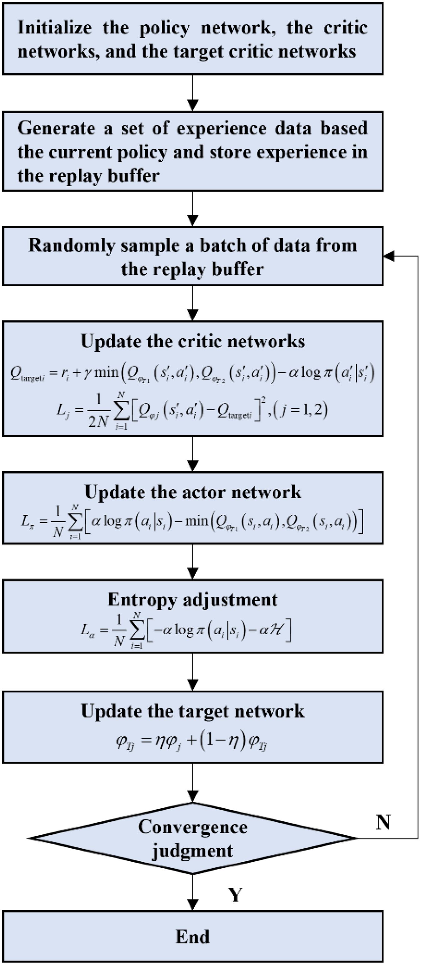
Figure 2. Parameter update process in the SAC-based actor-critic model.

Figure 3 provides a detailed visualization of the actor and critic networks. The critic network processes state and action inputs separately before combining them through concatenation and an LSTM layer for Q-value estimation. On the other hand, the actor network utilizes an LSTM layer to capture temporal features, followed by separate pathways for calculating the mean and standard deviation of the action distribution, ensuring a stochastic yet optimized policy. In the present application, the training process was conducted over 3000 episodes, with 1000 steps per episode.

Figure 3

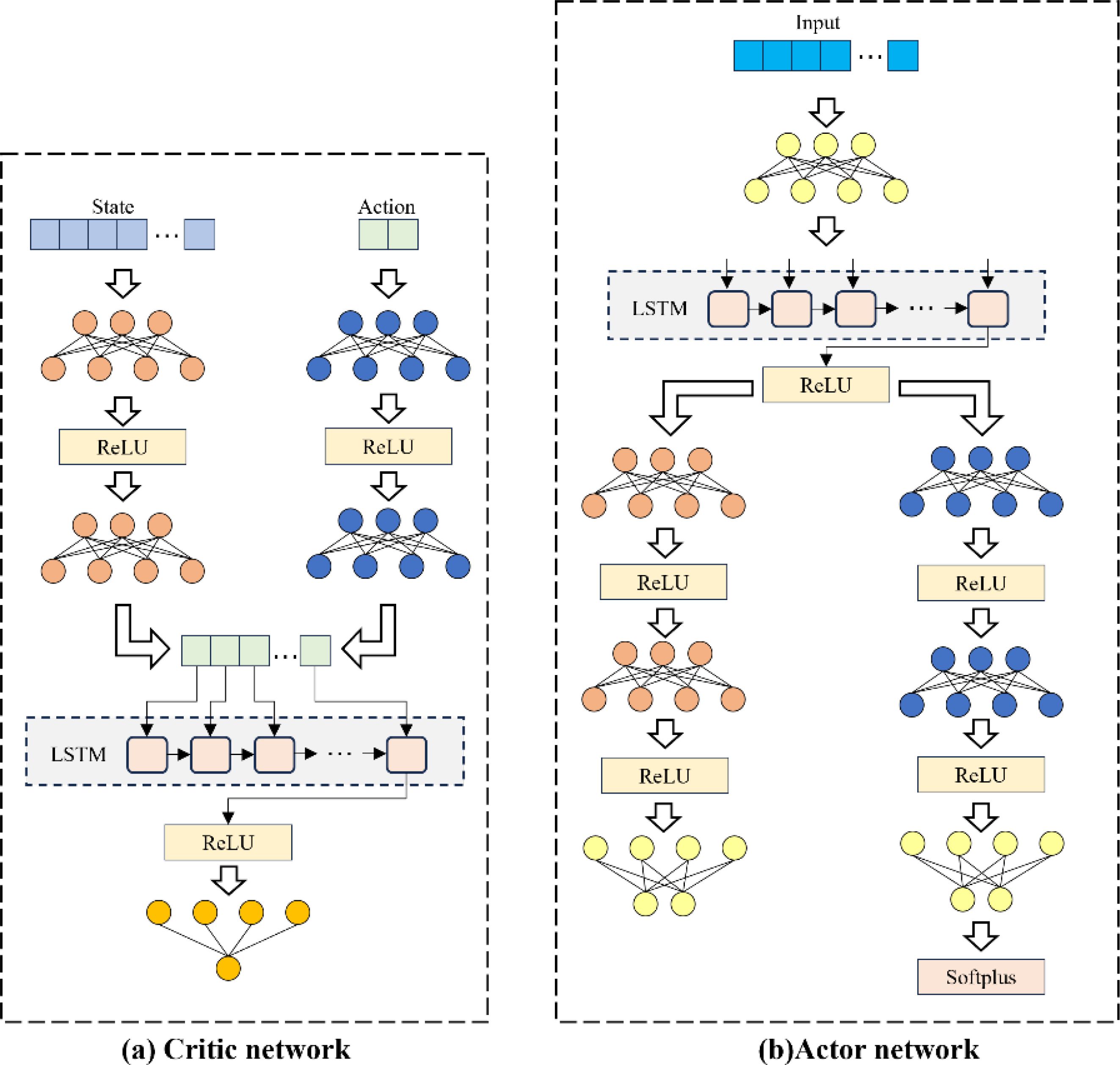
Figure 3. Network architecture of the actor-critic model ((A): critic network; (B): actor network).

3 Data description

To evaluate the effectiveness and applicability of the reinforcement learning-based model ensemble algorithm in ocean wave predictions, two distinct long-term wave field datasets along China’s coastline were used as base model outputs for the ensemble. These datasets were previously simulated using SWAN models by Yang et al. (2022) and Gong et al. (2022). The ERA5 reanalysis dataset was used as the reference standard. ERA5 is the fifth-generation reanalysis product developed by the European Centre for Medium-Range Weather Forecasts. Utilizing a four-dimensional variational analysis system, ERA5 integrates a wide range of measurements from multiple sources to enhance the accuracy and reliability of its data. The temporal and spatial resolutions for ocean waves are 1 hour and 0.5°×0.5°, respectively. ERA5 has been widely used as a reference dataset for wave characteristics analysis (Liu et al., 2024; Zhao J. et al., 2024). The study area focuses on the coastal regions of China, outlined by the red boundary in Figure 4. This area includes the Yellow Sea, East China Sea, and the northern part of the South China Sea, extending from the Beibu Gulf to the Bashi Strait.

Figure 4

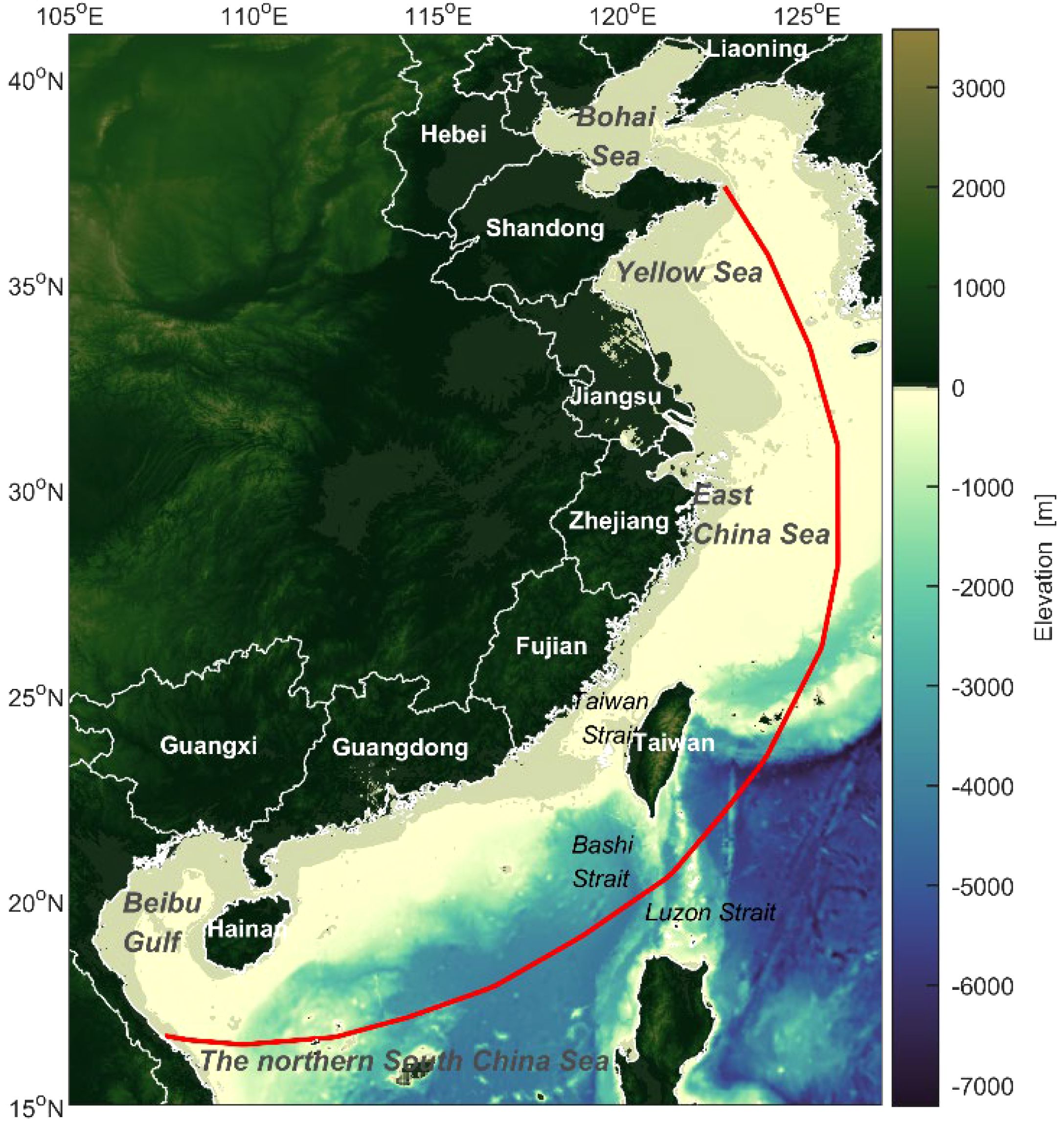
Figure 4. Study area along China’s coastline, with the red line indicating the boundary of the study region.

The SWAN-I model, established by Gong et al. (2022), incorporates typhoon effects by combining wind fields generated from a typhoon dynamical model with CFSR/CFSv2 reanalysis winds, weighted appropriately to capture both the intense wind conditions near typhoon centers and broader atmospheric patterns. This model features a two-layer nested structure, with the outer layer covering 105°E−140°E and 10°N−41°N, and a second layer covering 118°E−125°E and 24°N−30°N at a spatial resolution of 1′×1′. The second layer receives open boundary conditions from the outer layer. In wave field simulations, the SWAN-I model accounts for wave breaking, including whitecapping, bottom friction, and nonlinear interactions across both shallow and deep waters. The model operates at a temporal resolution of 20 minutes, producing simulation outputs every 3 hours.

The SWAN-II model, developed by Yang et al. (2022), includes a parameter sensitivity analysis based on observational data, with a primary focus on factors such as wind field and energy dissipation processes like whitecapping dissipation and bottom friction. This analysis enabled optimized adjustments to the model. The SWAN-II model uses an unstructured grid with a resolution ranging from 0.0241° to 0.3927°, and bathymetric data from the ETOPO1 global dataset at a resolution of 1′. Model settings include a two-dimensional nonstationary mode with a maximum of five iterations per time step. The wave spectrum is represented by the JONSWAP spectrum, with ERA5 wind data serving as the driving wind field. The open ocean boundary conditions are driven by IOWAGA data from the French Research Institute for Exploitation of the Sea, covering variables such as significant wave height, peak wave period, peak wave direction, and directional spreading coefficient. The computational time step is set at 10 minutes, with hourly outputs of wave parameters at each node.

The SWAN-I and SWAN-II models differ significantly in terms of wind field input, grid resolution, and typhoon coupling methods. Specifically, SWAN-I couples a typhoon numerical model with reanalysis wind data to better capture wind conditions, whereas SWAN-II uses observational data for parameter optimization. These diverse sources and configurations provide a valuable basis for testing the reinforcement learning algorithm’s ability to handle inconsistent data sources, complex environments, and long time-series data, thereby verifying its robustness and applicability in ocean simulations.

To ensure consistency across the SWAN-I, SWAN-II, and ERA5 reanalysis datasets, spatial and temporal resolutions were aligned. Spatially, data from both SWAN models were interpolated to match the ERA5 grid using two-dimensional linear interpolation. Temporally, data points at 0:00, 3:00, 6:00, 9:00, 12:00, 15:00, 18:00, and 21:00 were selected for analysis. Significant wave height data from numerical simulations conducted between 2011 and 2016 were used, with data from 2011 to 2015 serving as the training dataset and data from 2016 as the validation dataset.

4 Results and discussion

4.1 Performance evaluation of the reinforcement learning-based model ensemble algorithm

To evaluate the performance of the reinforcement learning-based model ensemble algorithm, a systematic analysis was conducted using the test dataset from 2016, comparing the model ensemble algorithm and the base models. Three performance metrics, the root mean square error (RMSE), mean absolute error (MAE), and bias (BIAS), were calculated for this assessment. In this study, BIAS is defined as the difference between the ERA5 reanalysis data and the model predictions, where a positive BIAS indicates that the model underestimates significant wave height, while a negative BIAS indicates overestimation. These metrics provide a comprehensive evaluation of each model’s predictive accuracy and ability to simulate wave fields, highlighting their strengths and limitations in handling complex ocean environment. Figures 5–7 show the spatial distribution of RMSE, MAE, and BIAS, respectively.

Figure 5

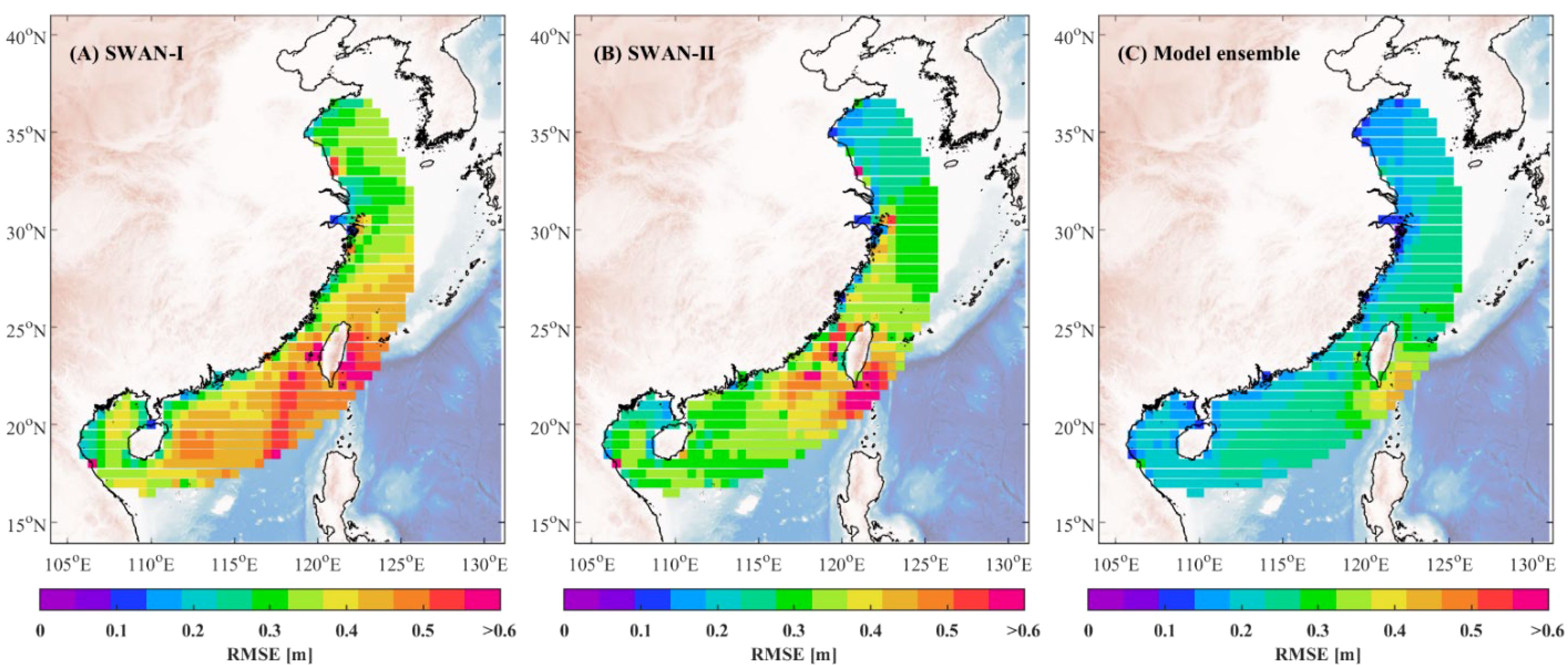
Figure 5. Spatial distribution of RMSE for SWAN-I model (A), SWAN-II model (B), and the model ensemble algorithm (C).

Figure 6

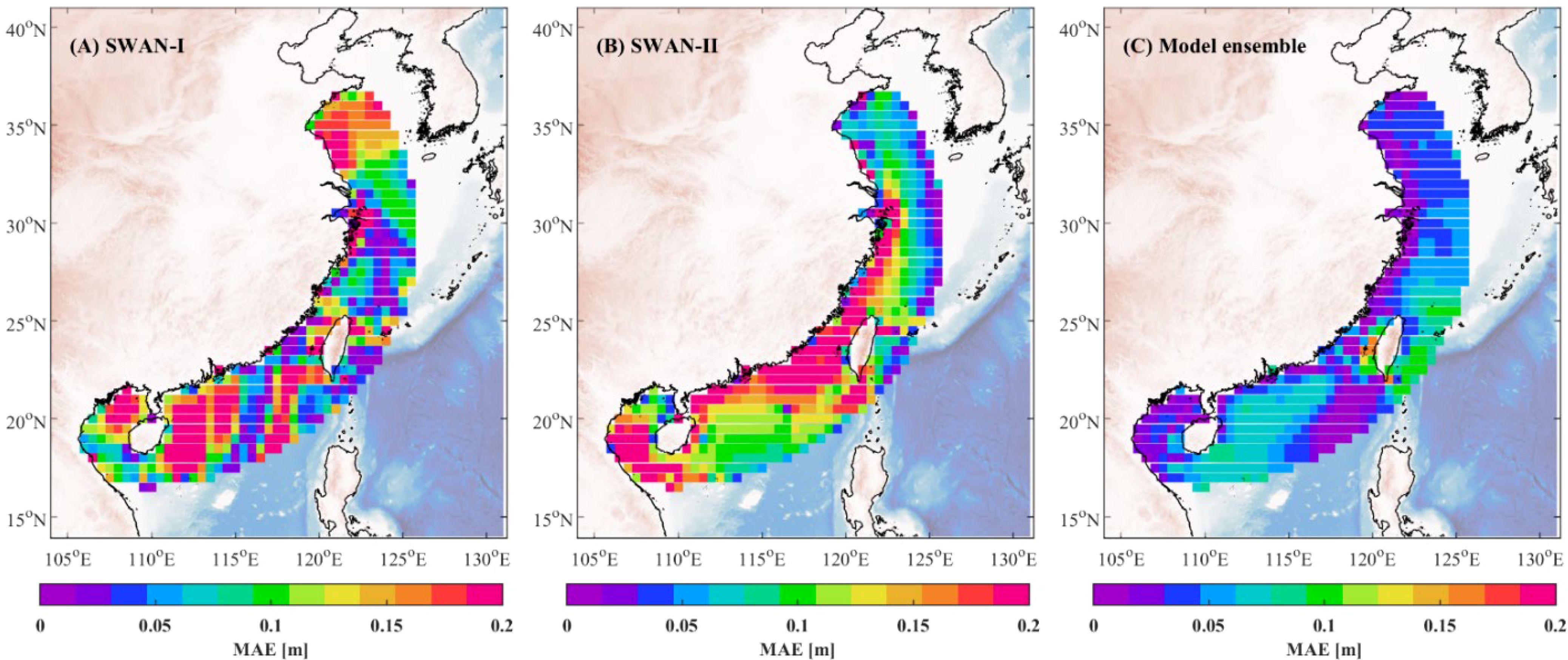
Figure 6. Spatial distribution of MAE for SWAN-I model (A), SWAN-II model (B), and the model ensemble algorithm (C).

Figure 7

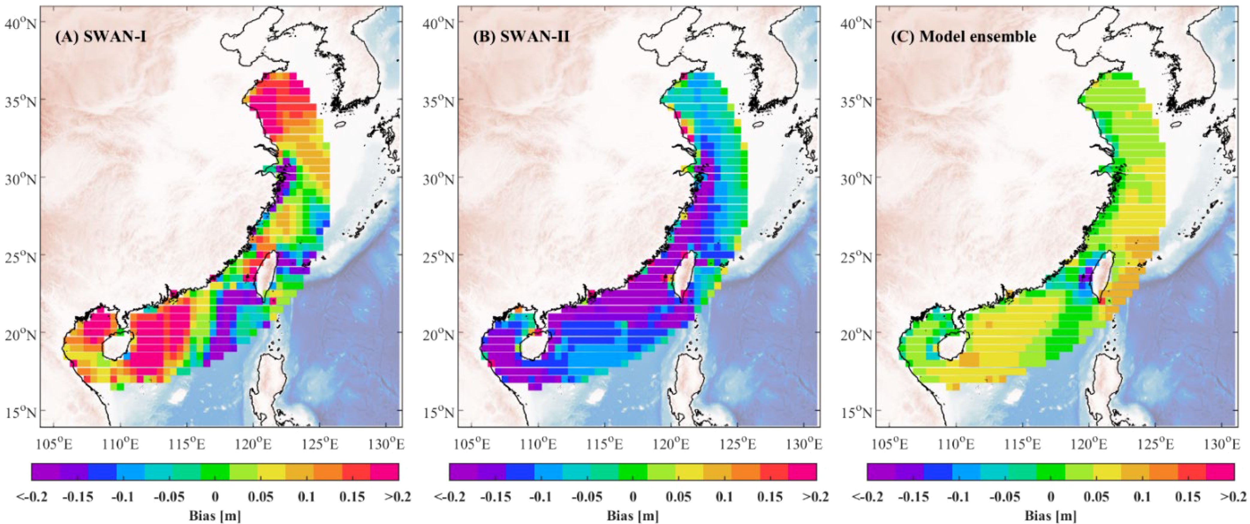
Figure 7. Spatial distribution of BIAS for SWAN-I model (A), SWAN-II model (B), and the model ensemble algorithm (C).

The RMSE comparison in Figure 5 indicates that the model ensemble algorithm consistently achieves lower RMSE values across the entire study area compared to the base models. High RMSE values are particularly evident in SWAN-I and SWAN-II models along the southern and eastern coastal regions of China, especially near Taiwan Island and parts of the South China Sea, where RMSE exceeds 0.6 meters. However, through the integration of both base models, the model ensemble algorithm effectively reduces these errors, resulting in more uniform RMSE values across the coastal region and significantly improving prediction accuracy. This suggests that the model ensemble algorithm is better suited to handle the diverse and complex ocean conditions in these areas.

The MAE comparison in Figure 6 further highlights the superior performance of the model ensemble algorithm, which consistently yields significantly lower MAE values across most regions compared to the SWAN-I and SWAN-II models. In areas with complex ocean dynamics, such as the Taiwan Strait, the base models exhibit MAE values exceeding 0.15 meters. In contrast, the ensemble model reduces these errors, with MAE values generally below 0.1 meters. This demonstrates the model ensemble algorithm’s enhanced adaptability and its ability to provide more consistent and accurate wave predictions. The improved capacity of the model ensemble algorithm to capture wave variations across different ocean conditions underscores its robustness and precision.

The BIAS comparison in Figure 7 reveals that both SWAN-I and SWAN-II models exhibit significant biases in certain regions, particularly in the South China Sea, indicating systematic overestimation or underestimation of significant wave heights. The SWAN-I model shows positive biases exceeding 0.2 meters in areas such as the eastern coast of Hainan Island and the southern region of Shandong Peninsula, while the SWAN-II model displays negative biases over a broader area. In contrast, the model ensemble algorithm substantially reduces bias, with BIAS values close to zero in most regions and a more uniform bias distribution. This demonstrates that the model ensemble algorithm’s ability to mitigate systematic errors, providing more accurate estimates of wave characteristics under varying spatiotemporal conditions.

Figures 8 and 9 further demonstrate the error reduction achieved by the model ensemble algorithm in terms of RMSE and MAE, respectively. The error reduction percentage ζ is calculated as shown in Equation 11:

Figure 8

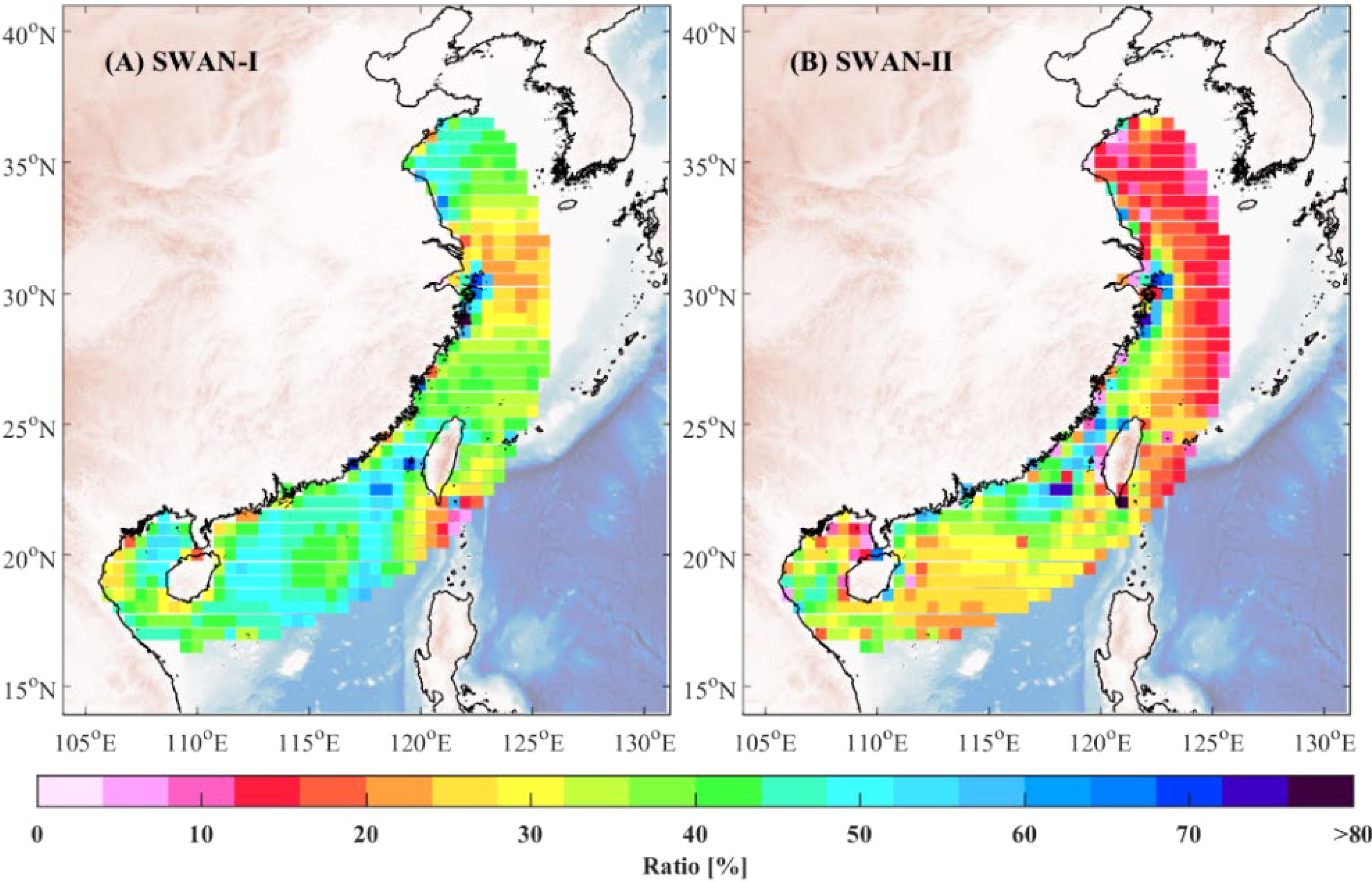
Figure 8. Spatial distribution of RMSE reduction percentage for model ensemble algorithm relative to SWAN-I (A) and SWAN-II (B) models.

Figure 9

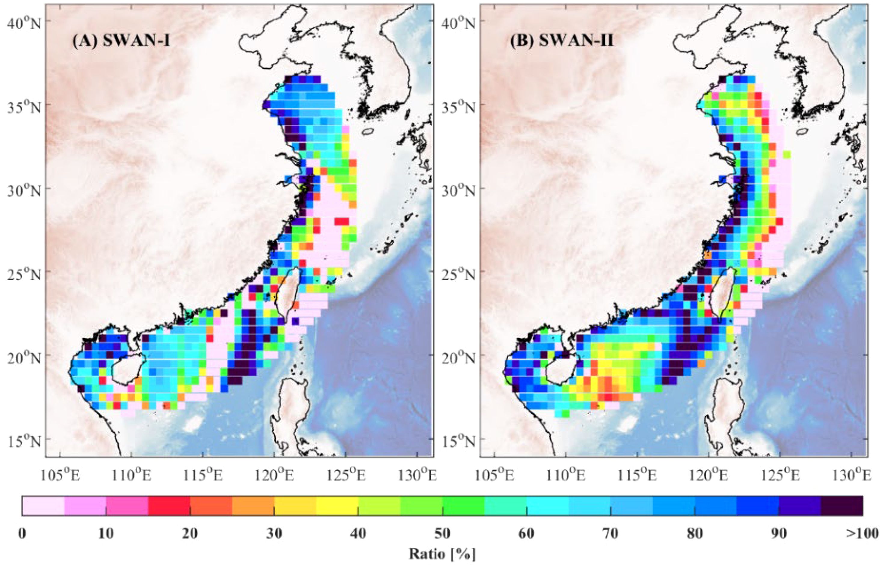
Figure 9. Spatial distribution of MAE reduction percentage for model ensemble algorithm relative to SWAN-I (A) and SWAN-II (B) models.

$\begin{array}{ll}\zeta =\frac{{\sigma }_{\text{base}}-{\sigma }_{\text{ensemble}}}{{\sigma }_{\text{base}}}\times 100\%& (11)\end{array}$

where σ_base and σ_ensemble represent the errors of base models and the model ensemble algorithm, respectively.

Figures 8A and Figures 8AB present the RMSE error reduction percentage achieved by the model ensemble algorithm relative to the SWAN-I and SWAN-II models, respectively. The results indicate that the model ensemble algorithm achieves significant error reductions across most regions. Notably, in parts of the South China Sea, the error reduction percentage exceeds 30%. Along the southeastern coast, the RMSE reduction surpasses 40% compared to both base models. These findings highlight the model ensemble algorithm’s ability to integrate the strengths of individual models, leading to a substantial decrease in prediction errors.

Similarly, Figures 9A and B illustrate the MAE error reduction percentage relative to the SWAN-I and SWAN-II models, respectively. Consistent with the RMSE results, the model ensemble algorithm demonstrates significant improvements in MAE across most regions. In many areas, the MAE reduction exceeds 50%, with reductions surpassing 80% in parts of the Taiwan Strait. This underscores the model ensemble algorithm’s capability to provide more stable and accurate predictions of wave variations, particularly in regions with complex wave dynamics.

The comparative analysis reveals that the reinforcement learning-based model ensemble algorithm consistently outperforms the base models on the test dataset. By combining the strengths of the SWAN-I and SWAN-II models, the model ensemble algorithm improves performance across diverse regions and ocean conditions. It not only reduces prediction errors but also substantially mitigates systematic biases. These results demonstrate that the model ensemble algorithm offers superior robustness and predictive accuracy when dealing with complex and dynamic ocean environments, making it a reliable tool for real-world applications such as marine engineering and disaster prevention.

4.2 Performance evaluation across different significant wave height ranges

To comprehensively assess the performance of the reinforcement learning-based model ensemble algorithm under various ocean conditions, this study analyzed its prediction accuracy within different significant wave height (H_s) ranges. Specifically, the significant wave heights were categorized into three ranges:

● Low H_s: 0−1 m

● Moderate H_s: 1−2 m

● High H_s: >2 m

This classification provides deeper insights into the algorithm’s performance and applicability across diverse marine environments, enabling an evaluation of its prediction accuracy at varying significant wave height levels. Such an analysis is crucial for understanding the algorithm’s adaptability and reliability under calm conditions, moderate sea states, and extreme weather scenarios. This evaluation is particularly relevant for practical applications, including ocean condition forecasting and the assessment of offshore operational safety. Figure 10 shows the spatial distribution of RMSE for the SWAN-I model, SWAN-II model, and the model ensemble algorithm within each significant wave height category.

Figure 10

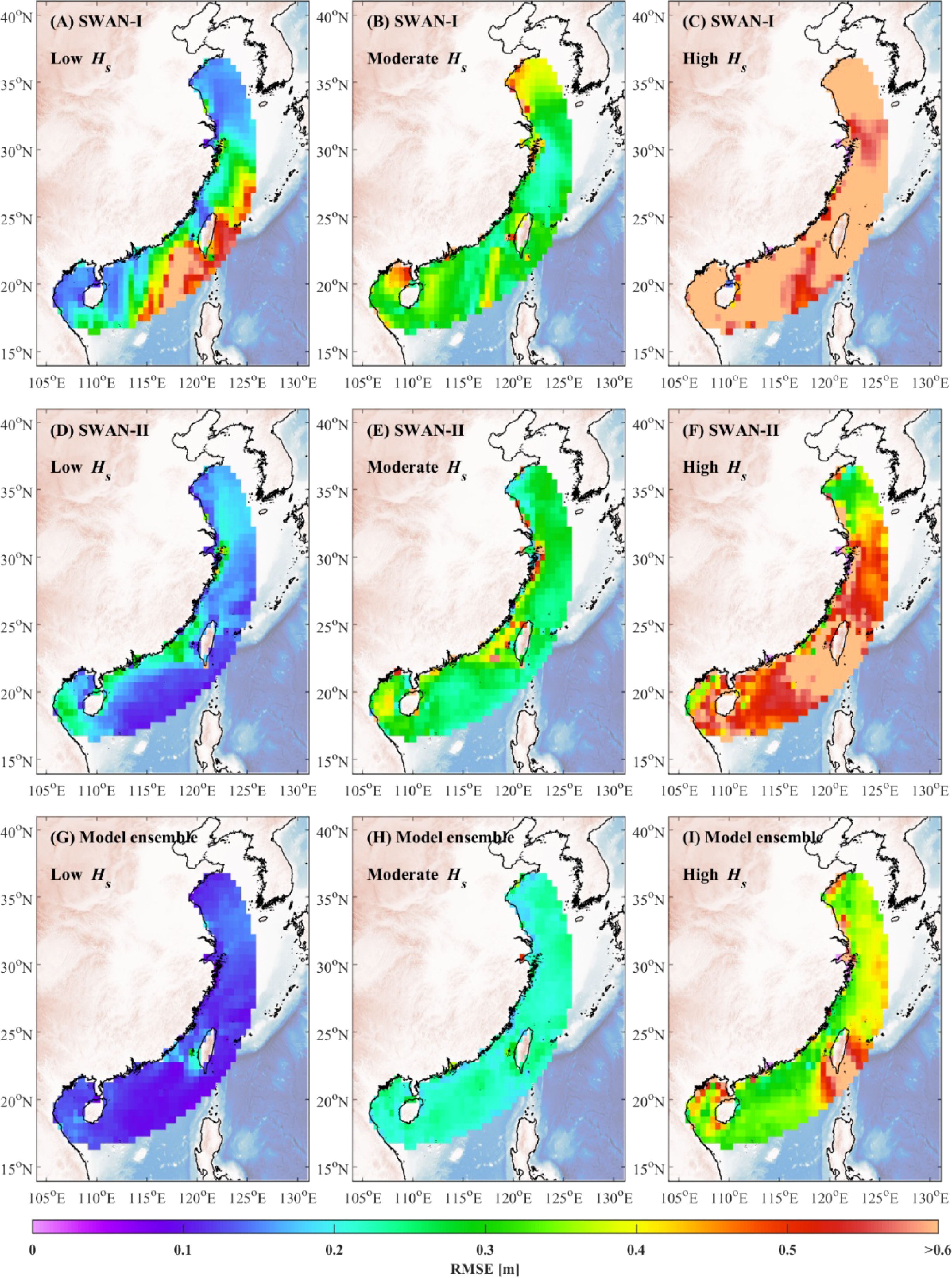
Figure 10. Spatial distribution of RMSE for the SWAN-I model (A–C), the SWAN-II model (D–F), and the model ensemble algorithm (G–I) across different significant wave height ranges.

Under low significant wave height conditions, notable differences in error distribution are observed between the SWAN-I and SWAN-II models, particularly near Taiwan Island. In this region, the SWAN-I model exhibits significant errors, while the SWAN-II model shows comparatively lower RMSE values. Overall, the model ensemble algorithm demonstrates a clear advantage in the low significant wave height range, consistently achieving lower errors than both base models. This improvement is particularly evident near Taiwan Island and along the southeastern coast of China, underscoring the model ensemble algorithm’s ability to reduce errors and provide more accurate predictions.

For moderate significant wave heights, errors increase for both the SWAN-I and SWAN-II models, especially along China’s eastern coastline, where RMSE values are relatively high. In certain areas, such as the coastal regions of Guangxi and Shandong, the SWAN-II model outperforms the SWAN-I model with lower RMSE values. However, the model ensemble algorithm significantly reduces errors across all regions, particularly in the eastern and southern nearshore areas of China. This demonstrates the model ensemble algorithm’s stability and accuracy in handling moderate wave height conditions.

In high significant wave height scenarios, both the SWAN-I and SWAN-II models exhibit increased errors across the study area, with RMSE values exceeding 0.5 meters in most regions. This can be attributed to the sensitivity of high wave conditions to boundary settings and the influence of nonlinear processes. While the model ensemble algorithm also experiences some errors under these conditions, its performance is generally superior to that of the SWAN-I and SWAN-II models. Notably, in the southern and eastern coastal regions of China, the model ensemble algorithm achieves lower errors, indicating its ability to maintain accuracy and enhance predictive performance even in challenging high wave scenarios.

The analysis across these three significant wave height ranges highlights that the model ensemble algorithm consistently outperforms the SWAN-I and SWAN-II models under low, moderate, and high wave conditions. This is particularly evident in regions with substantial error, such as near Taiwan Island. These improvements demonstrate the model ensemble algorithm’s capability to effectively integrate multiple data sources, reduce prediction errors, and enhance overall accuracy.

4.3 Performance evaluation under different base model error scenarios

To assess the performance of the model ensemble algorithm under varying base model error conditions, this study analyzed its behavior across different error combinations of the base models. Two scenarios were defined:

● Case 1: The error of the SWAN-I model is greater than that of the SWAN-II model.

● Case 2: The error of the SWAN-I model is less than that of the SWAN-II model.

This classification enables a detailed analysis of how the model ensemble algorithm’s performance varies depending on the relative accuracy of the base models. It also serves to further validate the model ensemble algorithm’s robustness and predictive capability under diverse error conditions. Figures 11, 12 present the RMSE distribution for the SWAN-I model, SWAN-II model, and model ensemble algorithm across these two base model error scenarios.

Figure 11

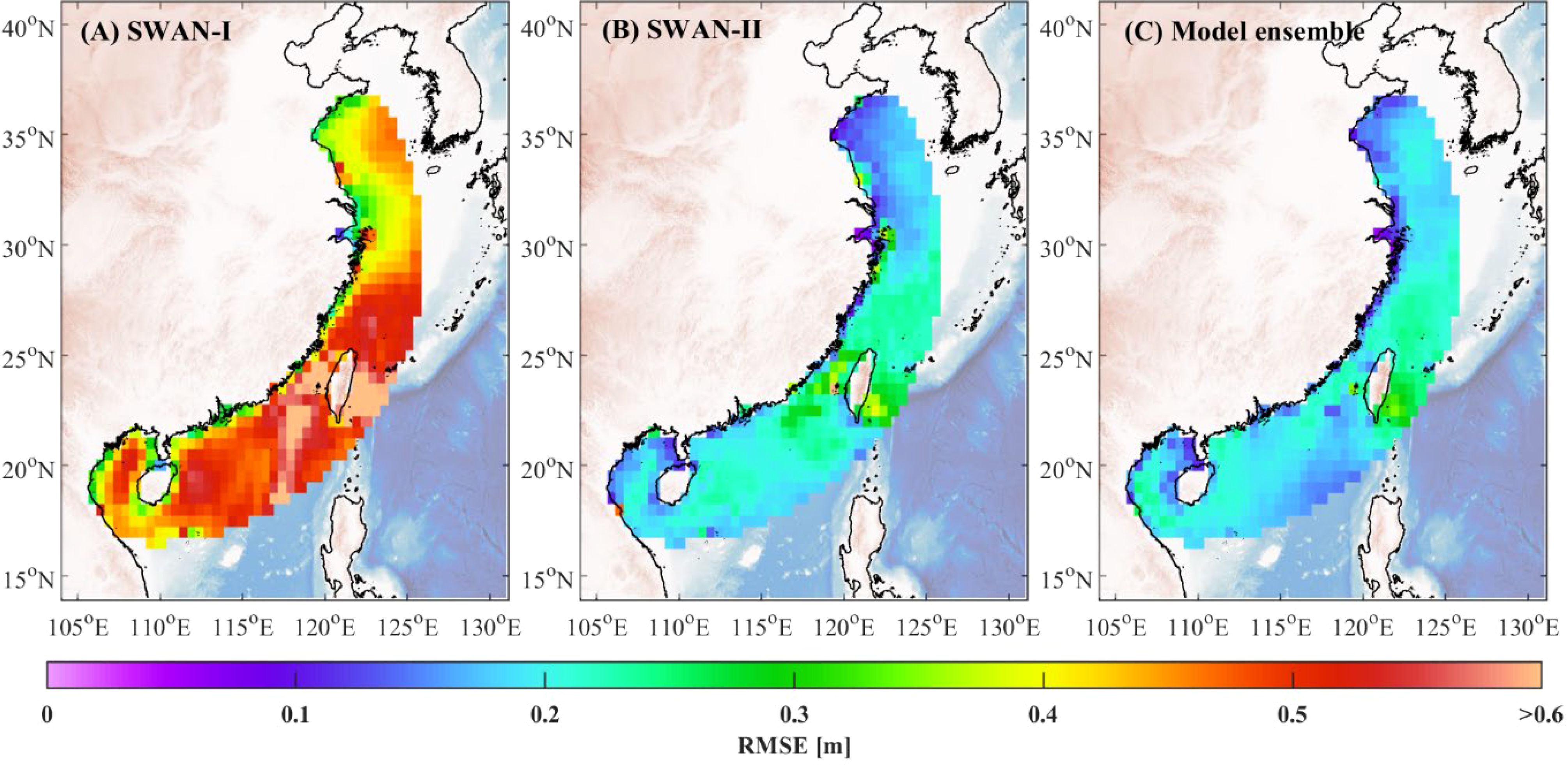
Figure 11. Spatial distribution of RMSE for the SWAN-I (A) model, the SWAN-II (B) model, and the model ensemble algorithm (C) model under Case 1.

Figure 12

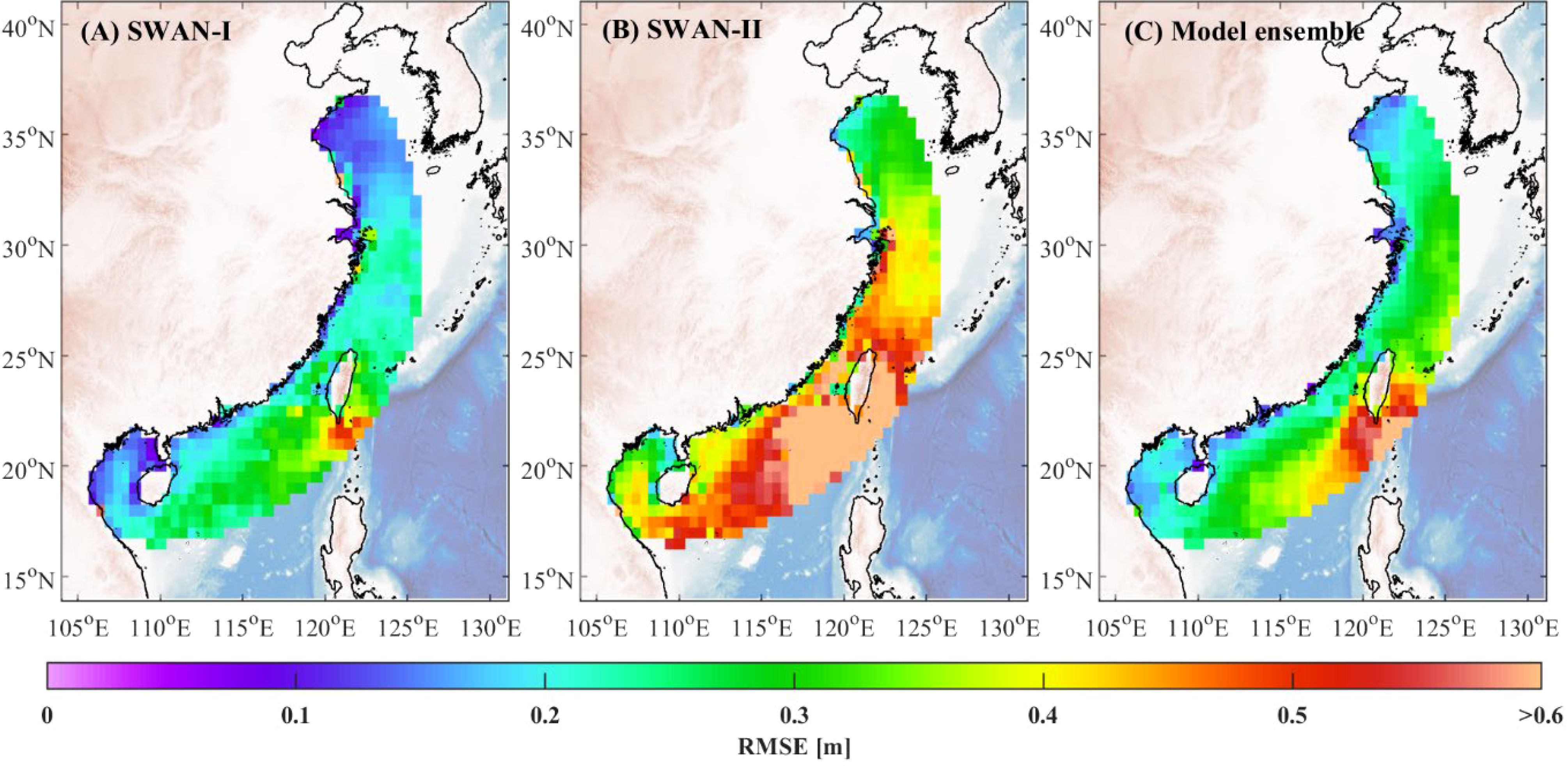
Figure 12. Spatial distribution of RMSE for the SWAN-I (A) model, the SWAN-II (B) model, and the model ensemble algorithm (C) model under Case 2.

The RMSE distribution for the model ensemble algorithm shows significant improvements in both scenarios. In Case 1, the model ensemble algorithm substantially reduces RMSE in areas where the SWAN-I model has high errors by effectively incorporating the superior performance of SWAN-II to minimize overall prediction errors. In Case 2, the model ensemble algorithm similarly achieves notable RMSE reductions, particularly in regions near Taiwan Island where the SWAN-II model exhibits high errors, by optimally weighting the contributions of both base models.

The comparison investigation reveals that the model ensemble algorithm consistently demonstrates robustness when faced with varying base model errors. Regardless of whether SWAN-I or SWAN-II exhibits higher errors, the model ensemble algorithm effectively optimizes predictions, achieving significantly lower RMSE across different regions. This indicates that the reinforcement learning-based ensemble algorithm can efficiently handle large discrepancies in base model performance. By effectively integrating the strengths of the individual models, the model ensemble algorithm mitigates the impact of high errors from any single base model, leading to improved prediction accuracy and reliability.

5 Conclusions

In this study, we proposed a reinforcement learning-based model ensemble algorithm aimed at improving the accuracy and robustness of ocean variable predictions by combining the outputs of multiple base models. The primary objective was to dynamically adjust the weights of each model, allowing the ensemble to utilize their respective strengths under varying conditions and generate more stable and precise predictions. By integrating the soft actor-critic reinforcement learning algorithm, the ensemble model adaptively optimizes the weights of the base models based on historical data and current environmental conditions.

To validate the proposed algorithm, two base models, SWAN-I and SWAN-II, were employed, focusing on China’s coastal regions, with ERA5 reanalysis data serving as the reference dataset. The results demonstrated that the model ensemble algorithm consistently outperformed the individual base models on the test dataset, showing significant improvements across multiple metrics, including RMSE, MAE, and BIAS.

Performance evaluation across different significant wave height ranges revealed that the model ensemble algorithm achieved superior predictive accuracy under low, moderate, and high wave height scenarios. This advantage was particularly evident in dynamic regions such the Taiwan Strait, where wave dynamics are highly complex. Furthermore, under varying base model error conditions, the model ensemble algorithm effectively reduced overall prediction errors through adaptive weight assignment, further highlighting its robustness.

This study demonstrates that reinforcement learning-based model ensemble algorithms provide significant advantages when dealing with complex ocean data. The proposed approach not only enhances the accuracy of wave field predictions but also substantially reduces systematic biases, showing high adaptability to diverse environmental conditions. Future research could extend this method to a broader range of ocean variables and explore other deep reinforcement learning techniques to further improve predictive performance and model generalization.

Data availability statement

Publicly available datasets were analyzed in this study. This data can be found here: Copernicus Climate Change Service.

Author contributions

WH: Writing – original draft, Writing – review & editing. XW: Writing – original draft, Writing – review & editing. HX: Writing – original draft, Writing – review & editing. XZ: Writing – original draft, Writing – review & editing. YG: Writing – original draft, Writing – review & editing. XS: Writing – original draft, Writing – review & editing.

Funding

The author(s) declare that financial support was received for the research, authorship, and/or publication of this article. The study was supported by the National Key Research and Development Program of China (2023YFC3008205), National Natural Science Foundation of China (52201339, 42377457), Natural Science Foundation of Shandong Province (ZR2022QE034), and Innovation Zone Program (22-05-CXZX-04-04-25).

Conflict of interest

The authors declare that the research was conducted in the absence of any commercial or financial relationships that could be construed as a potential conflict of interest.

Generative AI statement

The author(s) declare that no Generative AI was used in the creation of this manuscript.

Publisher’s note

All claims expressed in this article are solely those of the authors and do not necessarily represent those of their affiliated organizations, or those of the publisher, the editors and the reviewers. Any product that may be evaluated in this article, or claim that may be made by its manufacturer, is not guaranteed or endorsed by the publisher.

References

Ahmed K., Sachindra D. A., Shahid S., Demirel M. C., Chung E. S. (2019). Selection of multi-model ensemble of general circulation models for the simulation of precipitation and maximum and minimum temperature based on spatial assessment metrics. Hydrol. Earth Sys. Sci. 23, 4803–4824. doi: 10.5194/hess-23-4803-2019

Crossref Full Text | Google Scholar

Allahdadi M. N., He R., Neary V. S. (2019). Predicting ocean waves along the US east coast during energetic winter storms: Sensitivity to whitecapping parameterizations. Ocean Sci. 15, 691–715. doi: 10.5194/os-15-691-2019

Crossref Full Text | Google Scholar

Arulkumaran K., Deisenroth M. P., Brundage M., Bharath A. A. (2017). Deep reinforcement learning: A brief survey. IEEE Signal Process. Mag. 34, 26–38. doi: 10.1109/MSP.2017.2743240

Crossref Full Text | Google Scholar

Booij N. R. R. C., Ris R. C., Holthuijsen L. H. (1999). A third-generation wave model for coastal regions: 1. Model description and validation. J. Geophys. Res.: Oceans 104, 7649–7666. doi: 10.1029/98JC02622

Crossref Full Text | Google Scholar

Casas-Prat M., Hemer M. A., Dodet G., Morim J., Wang X. L., Mori N., et al. (2024). Wind-wave climate changes and their impacts. Nat. Rev. Earth Environ. 5, 23–42. doi: 10.1038/s43017-024-00518-0

Crossref Full Text | Google Scholar

Cavaleri L., Abdalla S., Benetazzo A., Bertotti L., Bidlot J. R., Breivik Ø., et al. (2018). Wave modelling in coastal and inner seas. Prog. Oceanogr. 167, 164–233. doi: 10.1016/j.pocean.2018.03.010

Crossref Full Text | Google Scholar

Cavaleri L., Fox-Kemper B., Hemer M. (2012). Wind waves in the coupled climate system. Bull. Am. Meteorol. Soc. 93, 1651–1661. doi: 10.1175/BAMS-D-11-00170.1

Crossref Full Text | Google Scholar

Christakos K., Björkqvist J. V., Tuomi L., Furevik B. R., Breivik Ø. (2021). Modelling wave growth in narrow fetch geometries: The white-capping and wind input formulations. Ocean Model. 157, 101730. doi: 10.1016/j.ocemod.2020.101730

Crossref Full Text | Google Scholar

Counillon F., Keenlyside N., Wang S., Devilliers M., Gupta A., Koseki S., et al. (2023). Framework for an ocean-connected supermodel of the earth system. J. Adv. Model. Earth Syst. 15, 2022MS003310. doi: 10.1029/2022MS003310

Crossref Full Text | Google Scholar

Dankwa S., Zheng W. (2019). Twin-delayed DDPG: A deep reinforcement learning technique to model a continuous movement of an intelligent robot agent. ICVISP 2019: Proceedings of the 3rd International Conference on Vision, Image and Signal Processing, Vancouver BC, Canada, August 26−28, 2019. Association for Computing Machinery, New York, United States. Vol. 66, 1–5. doi: 10.1145/3387168.3387199

Crossref Full Text | Google Scholar

Dey A., Sahoo D. P., Kumar R., Remesan R. (2022). A multimodel ensemble machine learning approach for CMIP6 climate model projections in an Indian River basin. Int. J. Climatol. 42, 9215–9236. doi: 10.1002/joc.7813

Crossref Full Text | Google Scholar

Duan Q., Ajami N. K., Gao X., Sorooshian S. (2007). Multi-model ensemble hydrologic prediction using Bayesian model averaging. Adv. Water Resour. 30, 1371–1386. doi: 10.1016/j.advwatres.2006.11.014

Crossref Full Text | Google Scholar

Duane G. S., Shen M. L. (2023). Synchronization of alternative models in a supermodel and the learning of critical behavior. J. Atmos. Sci. 80, 1565–1584. doi: 10.1175/JAS-D-22-0113.1

Crossref Full Text | Google Scholar

Fan J., Wang Z., Xie Y., Yang Z. (2020). “A theoretical analysis of deep Q-learning,” in Proceedings of the 2nd Conference on Learning for Dynamics and Control, June 10–11, 2020. The Cloud, Proceedings of Machine Learning Research, Vol. 120. 486–489. Cambridge MA: JMLR, United States.

Google Scholar

Fooladi M., Golmohammadi M. H., Safavi H. R., Singh V. P. (2021). Fusion-based framework for meteorological drought modeling using remotely sensed datasets under climate change scenarios: Resilience, vulnerability, and frequency analysis. J. Environ. Manage. 297, 113283. doi: 10.1016/j.jenvman.2021.113283

PubMed Abstract | Crossref Full Text | Google Scholar

Fu Y., Wu D., Boulet B. (2022). “Reinforcement learning based dynamic model combination for time series forecasting,” in Proceedings of the AAAI Conference on Artificial Intelligence. AAAI Press, Palo Alto, California, USA, 36 (6), 6639–6647. doi: 10.1609/aaai.v36i6.20618

Crossref Full Text | Google Scholar

Gentile E. S., Gray S. L., Barlow J. F., Lewis H. W., Edwards J. M. (2021). The impact of atmosphere–ocean–wave coupling on the near-surface wind speed in forecasts of extratropical cyclones. Boundary-Layer Meteorol. 180, 105–129. doi: 10.1007/s10546-021-00614-4

Crossref Full Text | Google Scholar

Gong Y., Wang Z., Dong S., Zhao Y. (2022). Coastal distributions of design environmental loads in typhoon-affected sea area based on the trivariate joint distribution and environmental contour method. Coast. Eng. 178, 104221. doi: 10.1016/j.coastaleng.2022.104221

Crossref Full Text | Google Scholar

Gronauer S., Diepold K. (2022). Multi-agent deep reinforcement learning: a survey. Artif. Intell. Rev. 55, 895–943. doi: 10.1007/s10462-021-09996-w

Crossref Full Text | Google Scholar

Grondman I., Busoniu L., Lopes G. A., Babuska R. (2012). A survey of actor-critic reinforcement learning: Standard and natural policy gradients. IEEE Trans. Sys. Man Cybernet. Part C (Applications Reviews) 42, 1291–1307. doi: 10.1109/TSMCC.2012.2218595

Crossref Full Text | Google Scholar

Group T. W. (1988). The WAM model—A third generation ocean wave prediction model. J. Phys. Oceanogr. 18, 1775–1810. doi: 10.1175/1520-0485(1988)018<1775:TWMTGO>2.0.CO;2

Crossref Full Text | Google Scholar

Haarnoja T., Zhou A., Abbeel P., Levine S. (2018). “Soft actor-critic: Off-policy maximum entropy deep reinforcement learning with a stochastic actor,” in Proceedings of the 35th International Conference on Machine Learning, July 10–15, 2018, Stockholmsmässan, Stockholm Sweden. Vol. 80. 1861–1870. Cambridge MA: JMLR, United States.

Google Scholar

Hagedorn R., Doblas-Reyes F. J., Palmer T. N. (2005). The rationale behind the success of multi-model ensembles in seasonal forecasting—I. Basic concept Tellus A: Dynam. Meteorol. Oceanogr. 57, 219–233. doi: 10.3402/tellusa.v57i3.14657

Crossref Full Text | Google Scholar

Kaelbling L. P., Littman M. L., Moore A. W. (1996). Reinforcement learning: A survey. J. Artif. Intell. Res. 4, 237–285. doi: 10.1613/jair.301

Crossref Full Text | Google Scholar

Krishnamurti T. N., Chakraborty A., Krishnamurti R., Dewar W. K., Clayson C. A. (2006). Seasonal prediction of sea surface temperature anomalies using a suite of 13 coupled atmosphere–ocean models. J. Climate 19, 6069–6088. doi: 10.1175/JCLI3938.1

Crossref Full Text | Google Scholar

Krishnamurti T. N., Kishtawal C. M., LaRow T. E., Bachiochi D. R., Zhang Z., Williford C. E., et al. (1999). Improved weather and seasonal climate forecasts from multimodel superensemble. Science 285, 1548–1550. doi: 10.1126/science.285.5433.1548

PubMed Abstract | Crossref Full Text | Google Scholar

Krishnamurti T. N., Kumar V., Simon A., Bhardwaj A., Ghosh T., Ross R. (2016). A review of multimodel superensemble forecasting for weather, seasonal climate, and hurricanes. Rev. Geophys. 54, 336–377. doi: 10.1002/2015RG000513

Crossref Full Text | Google Scholar

Kumar V., Krishnamurti T. N. (2012). Improved seasonal precipitation forecasts for the Asian monsoon using 16 atmosphere–ocean coupled models. Part I: Climatology. J. Climate 25, 39–64. doi: 10.1175/2011JCLI4125.1

Crossref Full Text | Google Scholar

Lenartz F., Mourre B., Barth A., Beckers J. M., Vandenbulcke L., Rixen M. (2010). Enhanced ocean temperature forecast skills through 3-D super-ensemble multi-model fusion. Geophys. Res. Lett. 37, L19606. doi: 10.1029/2010GL044591

Crossref Full Text | Google Scholar

Li S. E. (2023). “Deep Reinforcement Learning,” in Reinforcement Learning for Sequential Decision and Optimal Control (Springer, Singapore). doi: 10.1007/978-981-19-7784-8_10

Crossref Full Text | Google Scholar

Li D., Marshall L., Liang Z., Sharma A. (2022). Hydrologic multi-model ensemble predictions using variational Bayesian deep learning. J. Hydrol. 604, 127221. doi: 10.1016/j.jhydrol.2021.127221

Crossref Full Text | Google Scholar

Liang Z., Wei X., Sun X. (2022). An investigation into the variant-weight multi-model ensemble forecasting technique based on the analyses of model systematic errors calculation and elimination. Earth Space Sci. 9, EA002547. doi: 10.1029/2022EA002547

Crossref Full Text | Google Scholar

Lillicrap T. P., Hunt J. J., Pritzel A., Heess N., Erez T., Tassa Y., et al. (2015). Continuous control with deep reinforcement learning. arXiv preprint arXiv:1509.02971. doi: 10.48550/arXiv.1509.02971

Crossref Full Text | Google Scholar

Littardi A., Hildeman A., Nicolaou M. A. (2022). “Deep learning on the sphere for multi-model ensembling of significant wave height,” in 2022 IEEE International Conference on Acoustics, Speech and Signal Processing (ICASSP), May 23−27, 2022, Singapore. Institute of Electrical and Electronics Engineers (IEEE), New York, United States, 3828–3832. doi: 10.1109/ICASSP43922.2022.9747289

Crossref Full Text | Google Scholar

Liu Y., Lu W., Wang D., Lai Z., Ying C., Li X., et al. (2024). Spatiotemporal wave forecast with transformer-based network: A case study for the northwestern Pacific Ocean. Ocean Model. 188, 102323. doi: 10.1016/j.ocemod.2024.102323

Crossref Full Text | Google Scholar

Liu Q., Rogers W. E., Babanin A. V., Young I. R., Romero L., Zieger S., et al. (2019). Observation-based source terms in the third-generation wave model WAVEWATCH III: Updates and verification. J. Phys. Oceanogr. 49, 489–517. doi: 10.1175/JPO-D-18-0137.1

Crossref Full Text | Google Scholar

Mourre B., Chiggiato J. (2014). A comparison of the performance of the 3-D super-ensemble and an ensemble Kalman filter for short-range regional ocean prediction. Tellus A: Dynam. Meteorol. Oceanogr. 66, 21640. doi: 10.3402/tellusa.v66.21640

Crossref Full Text | Google Scholar

Nachum O., Norouzi M., Xu K., Schuurmans D. (2017). Bridging the gap between value and policy based reinforcement learning. Adv. Neural Inf. Process. Syst. 30. doi: 10.48550/arXiv.1702.08892

Crossref Full Text | Google Scholar

Peters J., Schaal S. (2008). Natural actor-critic. Neurocomputing 71, 1180–1190. doi: 10.1016/j.neucom.2007.11.026

Crossref Full Text | Google Scholar

Rascle N., Ardhuin F. (2013). A global wave parameter database for geophysical applications. Part 2: Model validation with improved source term parameterization. Ocean Model. 70, 174–188. doi: 10.1016/j.ocemod.2012.12.001

Crossref Full Text | Google Scholar

Reguero B. G., Losada I. J., Méndez F. J. (2019). A recent increase in global wave power as a consequence of oceanic warming. Nat. Commun. 10, 205. doi: 10.1038/s41467-018-08066-0

PubMed Abstract | Crossref Full Text | Google Scholar

Rixen M., Ferreira-Coelho E. (2007). Operational surface drift prediction using linear and non-linear hyper-ensemble statistics on atmospheric and ocean models. J. Mar. Syst. 65, 105–121. doi: 10.1016/j.jmarsys.2004.12.005

Crossref Full Text | Google Scholar

Rogers W. E., Van Vledder G. P. (2013). Frequency width in predictions of windsea spectra and the role of the nonlinear solver. Ocean Model. 70, 52–61. doi: 10.1016/j.ocemod.2012.11.010

Crossref Full Text | Google Scholar

Saadallah A., Morik K. (2021). “Online ensemble aggregation using deep reinforcement learning for time series forecasting,” in 2021 IEEE 8th International Conference on Data Science and Advanced Analytics (DSAA), Porto, Portugal, October 6–9, 2021. Porto, Portugal, Institute of Electrical and Electronics Engineers (IEEE), New York, United States. doi: 10.1109/DSAA53316.2021.9564132

Crossref Full Text | Google Scholar

Schevenhoven F., Keenlyside N., Counillon F., Carrassi A., Chapman W. E., Devilliers M., et al. (2023). Supermodeling: improving predictions with an ensemble of interacting models. Bull. Am. Meteorol. Soc. 104, E1670–E1686. doi: 10.1175/BAMS-D-22-0070.1

Crossref Full Text | Google Scholar

Schevenhoven F., Selten F., Carrassi A., Keenlyside N. (2019). Improving weather and climate predictions by training of supermodels. Earth Sys. Dynam. 10, 789–807. doi: 10.5194/esd-10-789-2019

Crossref Full Text | Google Scholar

Shin D. W., Krishnamurti T. N. (2003). Short-to medium-range superensemble precipitation forecasts using satellite products: 1. Deterministic forecasting. J. Geophys. Res.: Atmos. 108, 8383. doi: 10.1029/2001JD001510

Crossref Full Text | Google Scholar

Siadatmousavi S. M., Jose F., Da Silva G. M. (2016). Sensitivity of a third generation wave model to wind and boundary condition sources and model physics: A case study from the South Atlantic Ocean off Brazil coast. Comput. Geosci. 90, 57–65. doi: 10.1016/j.cageo.2015.09.025

Crossref Full Text | Google Scholar

Sutton R. S., Andrew G. B. (2018). Reinforcement Learning: An Introduction. 2nd ed. (Cambridge: The MIT Press).

Google Scholar

Tolman H. L. (1991). A third-generation model for wind waves on slowly varying, unsteady, and inhomogeneous depths and currents. J. Phys. Oceanogr. 21, 782–797. doi: 10.1175/1520-0485(1991)021<0782:ATGMFW>2.0.CO;2

Crossref Full Text | Google Scholar

Vandenbulcke L., Beckers J. M., Lenartz F., Barth A., Poulain P. M., Aidonidis M., et al. (2009). Super-ensemble techniques: Application to surface drift prediction. Prog. Oceanogr. 82, 149–167. doi: 10.1016/j.pocean.2009.06.002

Crossref Full Text | Google Scholar

Wang Y., Liu H., Zheng W., Xia Y., Li Y., Chen P., et al. (2019). Multi-objective workflow scheduling with deep-Q-network-based multi-agent reinforcement learning. IEEE Access 7, 39974–39982. doi: 10.1109/ACCESS.2019.2902846

Crossref Full Text | Google Scholar

Wang L., Ren H. L., Zhu J., Huang B. (2020). Improving prediction of two ENSO types using a multi-model ensemble based on stepwise pattern projection model. Climate Dynam. 54, 3229–3243. doi: 10.1007/s00382-006-0119-7

Crossref Full Text | Google Scholar

Yang Z., Lin Y., Dong S. (2022). Weather window and efficiency assessment of offshore wind power construction in China adjacent seas using the calibrated SWAN model. Ocean Eng. 259, 111933. doi: 10.1016/j.oceaneng.2022.111933

Crossref Full Text | Google Scholar

Yevnin Y., Toledo Y. (2022). A deep learning model for improved wind and consequent wave forecasts. J. Phys. Oceanogr. 52, 2531–2537. doi: 10.1175/JPO-D-21-0280.1

Crossref Full Text | Google Scholar

Zhao J., Guo Y., Lin Y., Zhao Z., Guo Z. (2024). A novel dynamic ensemble of numerical weather prediction for multi-step wind speed forecasting with deep reinforcement learning and error sequence modeling. Energy 302, 131787. doi: 10.1016/j.energy.2024.131787

Crossref Full Text | Google Scholar

Zhao G., Li D., Yang S., Qi J., Yin B. (2024). The development of a weather-type statistical downscaling model for wave climate based on wave clustering. Ocean Eng. 304, 117863. doi: 10.1016/j.oceaneng.2024.117863

Crossref Full Text | Google Scholar

Zhi X., Qi H., Bai Y., Lin C. (2012). A comparison of three kinds of multimodel ensemble forecast techniques based on the TIGGE data. Acta Meteorol. Sin. 26, 41–51. doi: 10.1007/s13351-012-0104-5

Crossref Full Text | Google Scholar