Characteristics and driving mechanisms of mixing and stratification in Suances estuary using the potential energy anomaly budget equation

The environmental variability of rivers and tides create complex mixing patterns, which modulate the estuarine ecosystem services. Therefore, a thorough understanding of these systems is vital, not only for their protection but also for their recovery. This study first applies a method to analyze the different mechanisms driving the mixing and stratification of the water column in Suances estuary, a small estuary with large intertidal zones, by using numerical modeling to calculate the potential energy anomaly (ϕ) and its derivative (ϕ_t). Numerical results show that Suances estuary presents an ellipse of mixing and stratification variability driven by, firstly, the river flow (seasonal cycle – monthly time scale), secondly, the tidal phase (ebb-flood cycle – diurnal time scale) and, lastly, the tidal magnitude (spring-neap cycle – fortnightly time scale). Furthermore, these results explicitly highlight how the driving mechanisms can vary for the same estuary geometry at different locations due to diurnal, fortnightly and seasonal changes in forcing. The predominant driving mechanisms in Suances estuary are straining (S) tending to stratify the estuary, river and tide advection (A) tending to mix it and non-linear straining (N), caused by contributions from intertidal areas that favor mixing or stratification according to the tidal cycles. Additionally, a threshold was found between the potential energy anomaly and the depth of the water column, confirming that there are limiting values of the potential energy anomaly depending on the depth that can develop in the estuary. This is especially significant in small and shallow estuaries, since maximum values of the potential energy anomaly will be obtained as a function of depth.

1 Introduction

Estuaries are ecosystems rich in biodiversity in which complex physical processes occur due to the confluence of fresh and saltwater (Burchard and Hofmeister, 2008), such as mixing and stratification. Mixing in estuaries is the result of a combination of small-scale turbulent diffusion and a larger-scale variation of the mean advective field velocities. Accordingly, the stratification and intensity of turbulence are much greater in estuaries than in oceanic environments, primarily due to the forcing from freshwater discharges and the complex topography (Geyer et al., 2008). Estuarine stratification is important because it inhibits vertical mixing, can lead to hypoxia in sub-pycnocline waters, and plays a critical role in salt balance (Valle-Levinson, 2010). This study has focused on narrow and shallow estuaries where astronomical tides and river discharges are the most important forcing factors (Peñas et al., 2013), applying, for the first time, the driving mechanisms of mixing and stratification in Suances estuary, a small estuary located in the north of Spain (Lupiola et al., 2023a, b). A small estuary can be defined as estuaries where the cross-sectional mixing is rapid, the fluctuations in salinity and turbidity are quick because of their short lengths, the tidal elevation can be taken to be constant along the estuary and they usually have short flushing times (Smith, 1977; Canton et al., 2012; Winterwerp and Wang, 2013; Winterwerp et al., 2013; Uncles et al., 2014; Marin Jarrin and Sutherland, 2022; Largier, 2023).

Numerous studies have analyzed the mixing processes that occur in estuaries due to the interaction of runoff and tides (Fischer et al., 1979; Geyer et al., 2008; Bárcena et al., 2015b; Khadami et al., 2022). Moreover, the dependence on salinity advection within the estuary itself due to differences in bathymetry directly affects the movement of internal estuarine currents (Ralston et al., 2010), which may result in mixing fronts varying three-dimensionally and not only two-dimensionally (Rijnsburger et al., 2018). This fact could be increased in estuaries that are relatively small, narrow, shallow, and with sharp bathymetric changes due to large intertidal zones, because these geometric features can modify the lateral and vertical stratification patterns (Ross et al., 2017).

Since the majority of estuaries around the world are small estuaries (e.g., Digby et al. (1998) found that approximately 60% of all estuaries in Australia are small coastal plain estuaries), further research of small estuarine systems in all climatic zones around the world is required to properly understand the hydrodynamic and mixing properties of these small systems (Trevethan and Chanson, 2009). Unfortunately, as conditions may vary from ebb to ebb, many different pathways to dilution may exist for a single system, depending on a variety of external forcing mechanisms, such as river and tide. This is why it is a tremendous observational challenge to resolve the estuarine mixing processes across the spatiotemporal scales necessary to accurately compare interconnected mixing processes acting in different regions of the estuary (Horner-Devine et al., 2015). Most small estuaries have a bathymetric variability at a range of spatial scales, so it would also be expected to have similar spatiotemporal variability of mixing (Geyer and MacCready, 2014). The mixing processes occur at spatial scales corresponding with the local salinity gradients at fronts. These frontal scales are on the order of decennial to hundreds of meters in short estuaries, suggesting further investigations with increased resolution are merited to characterize the flow and bathymetric features that are producing the locally enhanced mixing (Warner et al., 2020).

The potential energy anomaly (ϕ) and its derivative (${\varphi }_t$) are used to evaluate the competition between mixing and stratification in the water column and the processes that cause it. ϕ explains the amount of mechanical energy (per m³) required to reach a specific density profile in the water column with a given density profile. Simpson and Hunter (1974) advanced the localization and study of the mixing and stratification processes in the Irish Sea, assuming that only local tidal mixing opposes the establishment of stratification by the contribution of buoyancy at the surface. Simpson et al. (1977) suggested the use of the water column density potential as a measure of stratification, so that, in Simpson (1981), the energy potential equation is defined as displayed in Equation 1. In this case, there is no generalized differentiation between different types of stratifications, being considered a stratified or partially stratified flow when ϕ>0.

$\begin{array}{ll}\varphi =\frac{1}{H}{\int }_{-h}^{\text{η}}gz(\overline{\rho }-\rho )dz=-\frac{1}{H}{\int }_{-h}^{\text{η}}gz\widetilde{\rho }dz & (1)\end{array}$

where ρ is the vertical profile of densities over the water column H, with H = η+h, where η is the water surface and h is the bottom, z the vertical coordinate, g the acceleration of gravity and $\overline{\text{ρ}}$ is the average density at a depth defined as shown in Equation 2:

$\begin{array}{ll}\widetilde{\rho }=\rho -\overline{\rho }& (2)\end{array}$

where $\tilde{\rho }$ is the density fluctuation.

Later, Van Aken (1986) formulated a model describing the mixing due to tides and wind as well as terms describing the stabilizing power of surface heat fluxes and the different advective masses due to residual currents. Subsequently, de Boer et al. (2008) derived ϕ-equation in three dimensions assuming a constant water depth and zero density fluxes between surface and bottom. In the same year, Burchard and Hofmeister (2008) derived the ϕ-equation based on the dynamic equations for potential temperature and salinity, the continuity equation, and an equation of state for density. Both contributions used a simple numerical model to evaluate the relative importance of each term to identify the mechanisms that govern the competition between mixing and stratification in the water column. More recently, Hamada and Kim (2021) developed an adaptation to the model for the case where the tidal amplitude is very small compared to the water column thickness. With ${\varphi }_t$, a reference solution for completely quantifying the driving mechanisms of mixing and stratification from a numerical model is available, including most of the processes relevant for estuaries (de Boer et al., 2008). ϕ has been used in several studies on stratification processes in estuaries (de Boer et al., 2008; Horner-Devine et al., 2015; Holt et al., 2022), resulting in an easy-to-apply parameter that helps to explain clearly and concisely the stratification changes and their temporal and spatial evolution.

The aim of this study is to unravel the characteristics and driving mechanisms of mixing and stratification in Suances estuary by using, for the first time, a three-dimensional hydrodynamic model to calculate ϕ and ${\varphi }_t$. This study focused on a small estuary where astronomical tides and river discharges are the most important forcing factors, explaining the spatiotemporal mixing and stratification variability. The contents of this work are organized as follows: in section 2, the setup of the numerical model in the study area will be described. Next, the ϕ-equation, the ${\varphi }_t$-equation, and the description of all the terms will be shown. In sections 3 and 4 the results and the discussion of the application to the study area will be presented, respectively. Finally, the conclusions of the study will be highlighted in section 5.

2 Materials and methods

2.1 Study area and available data

The Suances Estuary (SE), a mesotidal estuary located on the Cantabrian coast of Spain, spans approximately 12 km in length and 150 m in average width, covering a surface area of 340 hectares. Notably, 76% of this area consists of intertidal zones. Bathymetrically, the main channel depth ranges from 1 to 8 meters, with intertidal zones elevated about 3.2 meters above mean sea level. The primary freshwater inputs to SE are the Saja and Besaya rivers, which drain a combined catchment area of 966.67 km². These rivers exhibit a rapid hydrological response due to their small surface area, short length, and steep slopes, with flow rates varying significantly from 1 to 600 m³/s.

The coastal sea adjacent to the estuary reaches a maximum depth of 43 meters. Historical land reclamation efforts have reduced the original estuarine area by 30%. Additionally, approximately 50% of the estuary is bordered by dikes, totaling over 13,000 meters in length. These structures, particularly the jetty constructed in 1878 at the estuary’s mouth, have significantly altered the estuary’s hydrodynamic conditions. Figure 1 illustrates the locations of these dikes (marked with a -1m elevation in blue) and the main channel, as well as the discharge point of a Wastewater Treatment Plant (WWTP). The WWTP discharge, simulated with a flow rate between 0.5 and 1.5 m³/s and a temperature 2°C higher than the river water, is monitored for its environmental impact. During the study, curvilinear coordinates are used, with ‘N’ representing the longitudinal (along-estuary) direction and ‘M’ the transverse (cross-estuary) direction. For further details on the SE, readers are referred to the works of Bárcena et al. (2012a, b, 2015b, 2016, 2017a, b).

Figure 1

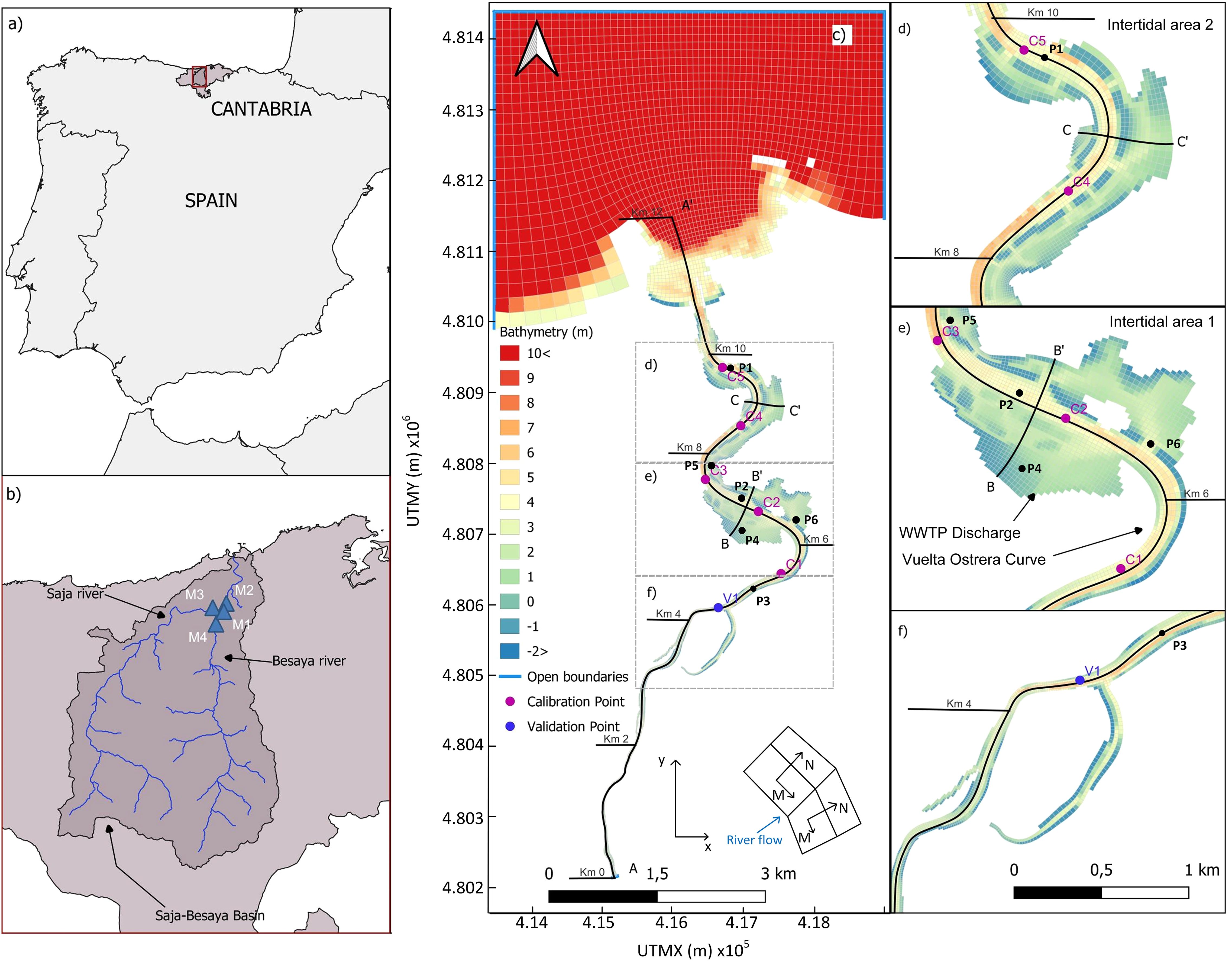
Figure 1. Location of (A) Cantabria in Spain and (B) Saja-Besaya river basin with the meteorological stations used in the study. (C) Bathymetry used in the 3D hydrodynamic model, the model mesh grid, and the open boundaries, zooming in on the central part of the estuary in panels (D–F). The following sections are marked: (D) C-C’ cross-estuary section at the intertidal zone 2; (E) B-B’ cross- section at the intertidal zone 1; and (C) A-A’ along-estuary section. Points C1 to C5 are the model calibration points and V1 is the model validation point. Note that x-direction and y-direction are referred to as eastward and northward direction, respectively. Moreover, the curvilinear coordinates are represented by the letters N in the longitudinal direction (along-estuary) and M in the transverse direction (cross-estuary).

2.2 Setup of the 3D hydrodynamic model

The 3D hydrodynamic model employed in this study was calibrated and validated by Lupiola et al. (2023a) using the three-dimensional option of the Delft3D-FLOW software (Nicholson et al., 1997; Lesser et al., 2004). This numerical model utilizes finite difference methods to solve the shallow water equations in three dimensions (Stelling, 1983), which are derived from the three-dimensional Navier–Stokes equations for free incompressible surface flow. For density calculations, the model incorporates the international standard formula of UNESCO (UNESCO, 1981). The Reynolds stress components are computed using the eddy viscosity concept (Rodi, 1987). The widespread use of this model globally has demonstrated its capability to accurately simulate 3D hydrodynamics in estuaries (García-Alba et al., 2014; Zapata et al., 2019).

The three-dimensional grid covering the SE and its adjacent coastal zone was represented horizontally using a curvilinear mesh grid consisting of 93 × 800 grid cells. The spatial resolution ranged from 47 to 235 meters in the adjacent coastal zone and from 4.3 to 30 meters within the estuary. Vertically, the mesh grid was composed of 20 equally spaced σ-layers along the water column, ensuring detailed capture of flows from the main channel to the intertidal zones. Calibration and validation of the model were conducted using data from points C1 to C5 and V1, as shown in Figure 1. Consequently, the study and numerical model are most accurate in the main channel.

The open boundaries correspond to the coastal zone and the limit of tidal influence (Figure 1), where tidal (level, temperature, and salinity) and river (flow, temperature, and salinity) forcings have been imposed, respectively. For more information about the model setup, calibration and validation, readers are referred to Supplementary Material 1, Lupiola et al., 2023a and Lupiola et al., 2023b.

2.3 Derivative of the potential energy anomaly equation

Following the steps of Simpson et al. (1990); de Boer et al. (2008), and Burchard and Hofmeister (2008), ${\varphi }_t$ is displayed in Equations 3–5, assuming the absence of source and sink terms such as surface heating, stirring and rain:

$\begin{array}{ll}{\varphi }_t=\frac{\partial \varphi }{\partial t}=\frac{g}{H}{\int }_{-h}^{\text{η}}(\frac{\partial \overline{\rho }}{\partial t}-\frac{\partial \rho }{\partial t})zdz& (3)\end{array}$

$\begin{array}{ll}\frac{\partial \rho }{\partial t}=-u\frac{\partial \rho }{\partial x}-v\frac{\partial \rho }{\partial y}= -(\overline{u}+\tilde{u})(\frac{\partial \overline{\rho }}{\partial x}+\frac{\partial \tilde{\rho }}{\partial x})-(\overline{v}+\tilde{v})(\frac{\partial \overline{\rho }}{\partial y}+\frac{\partial \tilde{\rho }}{\partial y})& (4)\end{array}$

$\begin{array}{ll}\frac{\partial \overline{\rho }}{\partial t}=-\overline{u}\frac{\partial \overline{\rho }}{\partial x}-\overline{v}\frac{\partial \overline{\rho }}{\partial y}& (5)\end{array}$

where t is the time, while $\overline{u}$ and $\overline{v}$, $\tilde{u}$ and $\tilde{v}$, $\frac{\partial \overline{\rho }}{\partial x}$ and $\frac{\partial \overline{\rho }}{\partial y}$, and $\frac{\partial \tilde{\rho }}{\partial x}$ and $\frac{\partial \tilde{\rho }}{\partial y}$ are the depth-averaged horizontal velocity, the deviation from depth-averaged horizontal velocity, the depth-averaged density gradient, and the vertical deviation of the density gradient in x-direction and y-direction, respectively.

Next, ${\varphi }_t$ is decomposed into different terms (mechanisms) as defined by de Boer et al. (2008) and shown in Equation 6.

$\begin{array}{ll}\frac{\partial \varphi }{\partial t}=S_x+S_y+A_x+A_y+N_x+N_y+C_x+C_y+W_z+M_z+D_x+D_y+D_s+D_b+B_H+B_{\text{η}}& (6)\end{array}$

being each value represented by Equations 7–22:

$\begin{array}{ll}{S}_x=\frac{g}{H}{\int }_{-h}^{\text{η}}\tilde{u}\frac{\partial \overline{\rho }}{\partial x}zdz& (7)\end{array}$

$\begin{array}{ll}{S}_y=\frac{g}{H}{\int }_{-h}^{\text{η}}\tilde{v}\frac{\partial \overline{\rho }}{\partial y}zdz& (8)\end{array}$

$\begin{array}{ll}{A}_x=\frac{g}{H}{\int }_{-h}^{\text{η}}\overline{u}\frac{\partial \tilde{\rho }}{\partial x}zdz& (9)\end{array}$

$\begin{array}{ll}{A}_y=\frac{g}{H}{\int }_{-h}^{\text{η}}\overline{v}\frac{\partial \tilde{\rho }}{\partial y}zdz& (10)\end{array}$

$\begin{array}{ll}{N}_x=\frac{g}{H}{\int }_{-h}^{\text{η}}\tilde{u}\frac{\partial \tilde{\rho }}{\partial x}zdz& (11)\end{array}$

$\begin{array}{ll}{N}_y=\frac{g}{H}{\int }_{-h}^{\text{η}}\tilde{v}\frac{\partial \tilde{\rho }}{\partial y}zdz & (12)\end{array}$

$\begin{array}{ll}{C}_x=-\frac{g}{H}{\int }_{-h}^{\text{η}}\frac{1}{H} \frac{\partial \overline{\tilde{u}\tilde{\rho }}H}{\partial x}zdz& (13)\end{array}$

$\begin{array}{ll}{C}_y=-\frac{g}{H}{\int }_{-h}^{\text{η}}\frac{1}{H} \frac{\partial \overline{\tilde{v}\tilde{\rho }}H}{\partial y}zdz& (14)\end{array}$

$\begin{array}{ll}{W}_z=\frac{g}{H}{\int }_{-h}^{\text{η}}w\frac{\partial \rho }{\partial z}zdz& (15)\end{array}$

$\begin{array}{ll}{M}_z=\frac{g}{H}{\int }_{-h}^{\text{η}}\frac{\partial \langle {\rho }^{\prime }{w}^{\prime }\rangle }{\partial z}zdz& (16)\end{array}$

$\begin{array}{ll}{D}_x={\int }_{-h}^{\text{η}}\frac{\partial \langle {\rho }^{\prime }{u}^{\prime }\rangle }{\partial x}zdz& (17)\end{array}$

$\begin{array}{ll}{D}_y={\int }_{-h}^{\text{η}}\frac{\partial \langle {\rho }^{\prime }{v}^{\prime }\rangle }{\partial y}zdz& (18)\end{array}$

$\begin{array}{ll}{D}_s=-{\int }_{-h}^{\text{η}}\frac{1}{H}\langle {\rho }^{\prime }{w}^{\prime }\rangle {|}_{s}zdz& (19)\end{array}$

$\begin{array}{ll}{D}_b={\int }_{-h}^{\text{η}}\frac{1}{H}\langle {\rho }^{\prime }{w}^{\prime }\rangle {|}_{b}zdz& (20)\end{array}$

$\begin{array}{ll}{B}_H=-\frac{\phi }{H}\frac{\partial H}{\partial t}& (21)\end{array}$

$\begin{array}{ll}{B}_{\text{η}}=-(\frac{g}{H})(\tilde{\rho }(\text{η})\text{η}\frac{\partial \text{η}}{\partial t})& (22)\end{array}$

where the depth-averaged values ($\overline{\rho }$, $\overline{u}$, and $\overline{v}$) are ${\int }_{-h}^{\text{η}}\rho , u, v dz$, and the values of the fluctuations ($\tilde{\rho }$, $\tilde{u}$, and $\tilde{v}$) are obtained from the subtraction of the instantaneous values minus the depth-averaged values as presented in Equation 2.

As mentioned above, it is very important to highlight that we are using a curvilinear mesh grid adapted to the estuarine flow main direction (see Figure 1), being the N-coordinate the longitudinal direction (along-estuary) and the M-coordinate the transverse direction (cross-estuary). Accordingly, the analysis of terms in Equation 6 will give much more insight and make the results about the estuarine driving mechanism far more valuable by defining these directions in streamwise (N-coordinate) and spanwise (M-coordinate) direction or along (N-coordinate) and across (M-coordinate) the thalweg or centerline of the estuary (see Figure 1). For instance, if the velocity decomposition were North and East ($y$-direction and $x$-direction), then results will not give information on the quality of lateral flows, as $u_x$, $u_y$, $v_x$, and $v_y$, will be dominated by the longitudinal flow (see Figure 1). This is why ${\varphi }_t$ terms are computed considering the orthogonal curvilinear coordinates whose velocity decomposition has been obtained from numerical model along ($u_N$, $v_N$), and across ($u_M$, $v_M$), the thalweg or centerline of the estuary for every grid cell (see Figure 1).

Figure 2 shows a schematic sketch of each of ${\varphi }_t$ terms to help in the understanding of their physical meaning. In Figure 2, two diagrams can be seen for each mechanism. The left sketch shows the initial situation with the forcing that will activate the driving mechanism. In the right sketch, the effect that the driving mechanism generates in the water column can be seen. For every driving mechanism, this effect can favor the mixing or the stratification depending on the velocity and density field. In order to differentiate the effect generated by each driving mechanism, the contribution of each driving mechanism is identified by its sign, being positive for stratification and negative for mixing. Within this same figure, the forcings that act by each driving mechanism can be seen. The most important forcings are the average velocity, in red, the fluctuation of the velocity, in green, and the differences in densities, represented by the colors dark blue, grey and light blue, symbolizing from more to less density, respectively. In addition, the rest of the forcings that can act on the mixing and stratification in the water column are shown, such as the vertical velocity, w, in black, the lateral and vertical density fluxes, shown by curved arrows, and the changes in density, represented by orange arrows.

Figure 2

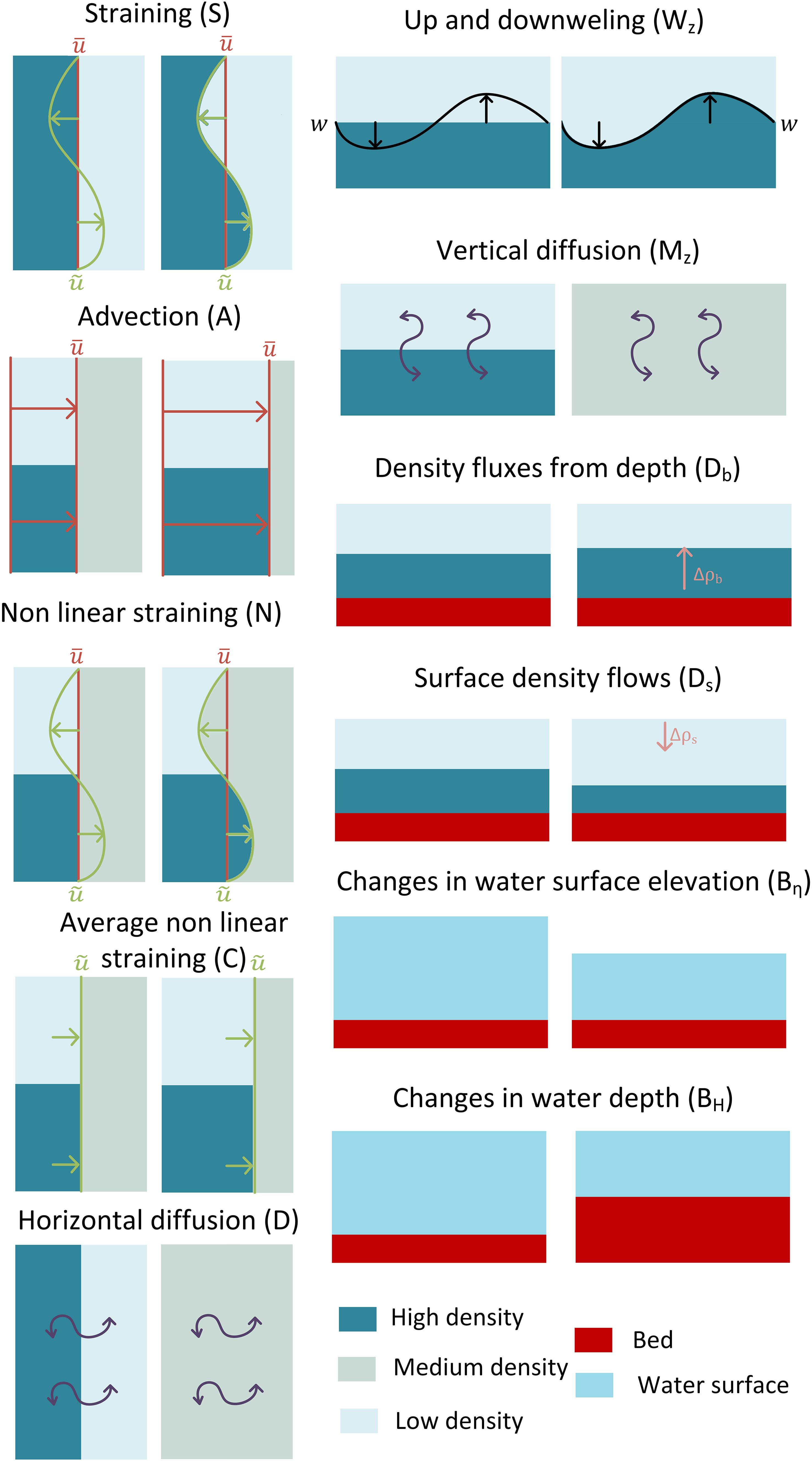
Figure 2. Conceptual scheme of the driving mechanisms involved in the derivative of ϕ (${\varphi }_t$).

The S_N and S_M driving mechanisms, respectively known as longitudinal and transversal tidal straining terms (S), originate because of the fluctuation of the velocity along the vertical profile, which generates a velocity shear that causes a deformation of the depth-averaged horizontal density gradient. This is caused by the confluence of two water masses of different densities which, when they meet with opposite velocities, produce these velocity fluctuations. A diagram of this effect can be seen in Figure 2, where it is possible to observe the encounter between freshwater flowing through the upper part and a denser water flowing through the lower part. This entry in opposite directions of both masses generates velocity fluctuations in the opposite direction, which causes the two masses of water of different salinity to mix or stratify.

The A_N and A_M driving mechanism are referred to longitudinal and transversal advection terms (A), respectively. They describe the thrust effect produced by the depth-averaged velocity current on a vertically fluctuating density profile. For example, these terms represent a profile of different densities that are displaced without deformation by the advective effect of an average velocity. Thus, this effect can be caused by the displacement of a stratified front in the estuary through a zone of flow acceleration, which due to the increase in velocity causes the fully stratified front to move. On the other hand, this effect can also occur in the opposite direction, since it can also push a homogeneous density front into a stratified zone.

The N_N and N_M driving mechanisms describe the longitudinal and transversal non-linear interaction between density deviation and velocity deviation about the vertical (N), respectively, i.e., it defines a joint effect of velocity shear and vertical variation of the density profile. This driving mechanism will be of particular attention where significant velocity and density gradient fluctuations occur, such as in areas where secondary density inputs are found, e.g., intertidal areas, which makes this mechanism relevant. The C_N and C_M driving mechanisms are homologous to N_N and N_M but vertically averaged (C). In this way, they show the vertical averaging of the longitudinal and transversal non-linear variation, originated by horizontal vortices in which the variation advances as a turbulent wake.

The W_z driving mechanism refers to “upwelling and downwelling” which describes the mixing of the denser bottom waters with the less dense top waters caused by the vertical velocity. The M_z driving mechanism describes the vertical diffusion originating from the vertical density fluxes, while D_N and D_M represent the longitudinal and transversal diffusion of the horizontal density flux averaged over depth (D), respectively. Driving mechanisms D_s and D_b are the surface density and bed density fluxes, respectively. Finally, the B_h and B_η driving mechanisms are due to changes in water depth or water surface elevation over time, respectively.

According to de Boer et al. (2008), some terms in Equation 8 are negligible compared to the magnitude of the effects generated by the S, A, N, C, and W_z driving mechanisms. For this reason, they can be combined into a single term that groups all these residual driving mechanisms together called “RESIDUE” and identified by the symbol Γ (Equation 23).

$\begin{array}{ll}\Gamma =M_z+D_M+D_N+D_s+D_b+B_H+B_{\text{η}}& (23)\end{array}$

Therefore, the derivative of ϕ (${\varphi }_t$) can be estimated according to Equation 24:

$\begin{array}{ll}{\varphi }_t=\frac{\partial \varphi }{\partial t}=S_M+S_N+A_M+A_N+N_M+N_N+C_M+C_N+W_z+\Gamma & (24)\end{array}$

2.4 Methodology to analyze the mechanisms driving the mixing and stratification

For the determination of $\varphi$ and ${\varphi }_t$, the previously calibrated and validated 3D hydrodynamic model was used. The analysis of the mechanisms driving the competition between mixing and stratification in estuaries is performed by the four-tiered method presented in Figure 3. In Tier 1, a high spatial resolution 3D hydrodynamic model is calibrated and validated (see section 2.2). Then, in Tier 2, $\varphi$ and ${\varphi }_t$ are calculated for every grid cell at each time step, one hour in this study. In Tier 3, $\varphi$ and the driving mechanisms are spatiotemporally analyzed by the time series and covariance methods, respectively. Lastly, in Tier 4, the most probable and persistent driving mechanisms are calculated, the negligible driving mechanisms are checked, and the zoning of mixing and stratification areas by mechanism is determined.

Figure 3

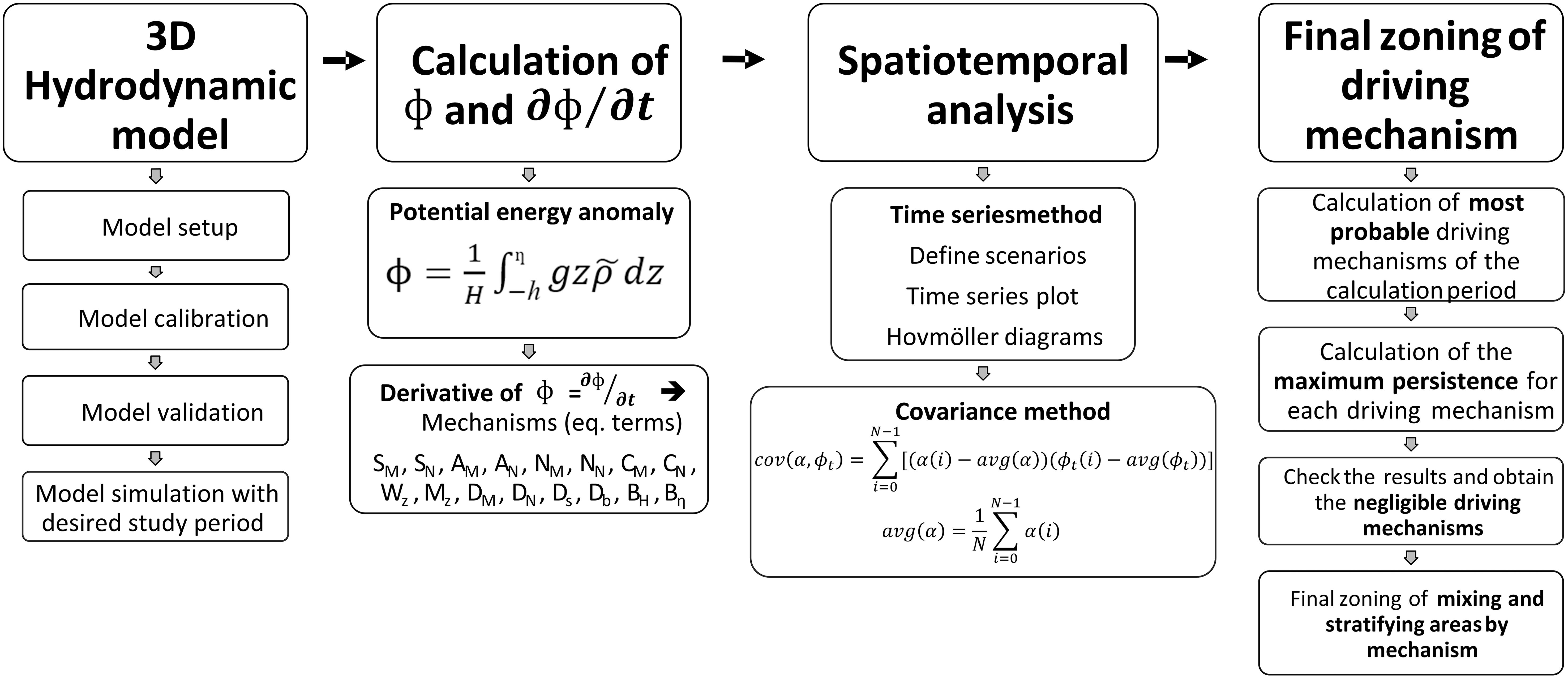
Figure 3. Methodology to analyze the mechanisms driving the competition between mixing and stratification in estuaries.

Firstly, after modeling the desired period in Tier 1 (one year in this study), the stratification fronts in the SE were analyzed by calculating $\varphi$ in Tier 2. Analogously, we proceeded to analyze $\partial \varphi /\partial t$ in their different terms to establish the driving mechanisms for every situation (temporal scale) and estuarine area (spatial scale) during the desired period.

Then, in Tier 3, we defined seven scenarios (time periods) representing the shifts experienced by the estuarine hydrodynamics in the desired period: (1) a neap tide and low flow event; (2) a spring tide and low flow event; (3) a neap tide and intermediate flow event; (4) a spring tide and intermediate flow event; (5) a neap tide and high flow event and (6) a spring tide and high flow event and (7) the desired period (see Table 1). In this study the desired period matches with the year 2020, which corresponds to a mean hydrological year with a mean annual water volume of 780 Hm³ (Bárcena Gómez, 2015a). Next, two methods were adopted to analyze the seven representative scenarios. The first was the time series method in which the instantaneous terms were plotted at a selected location and time step. The second was the covariance method in which the covariance between a term α and ${\varphi }_t$ was calculated, as discussed in section 2.4.

Table 1

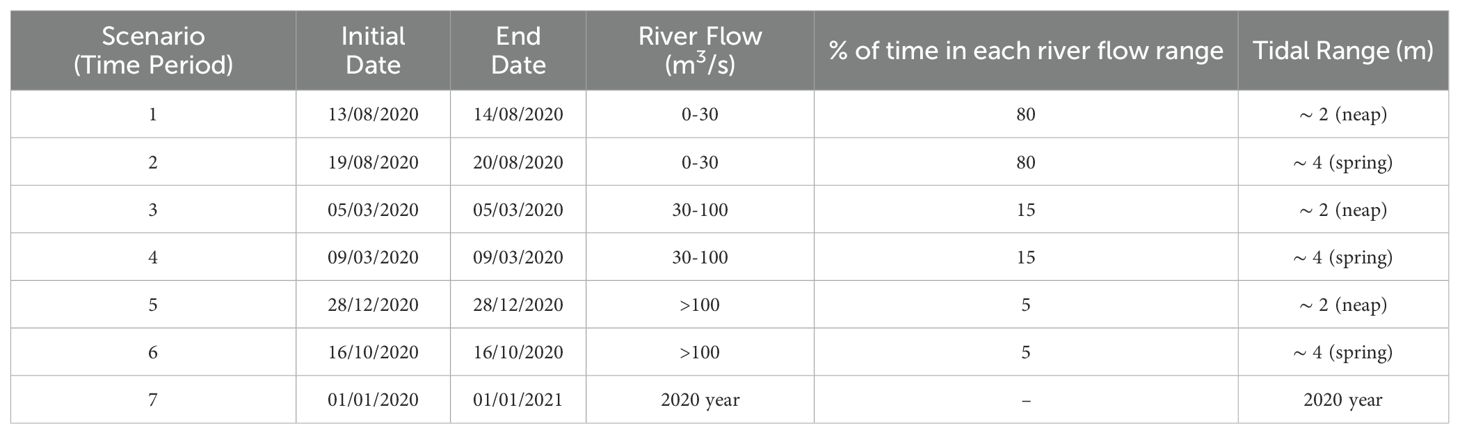
Table 1. Initial date, end date, river flow, % of time in each river flow range, and tidal range for the seven representative scenarios (time periods) in Suances estuary.

In Tier 4, the final zoning was conducted using two distribution maps: (1) the most probable driving mechanism and (2) the most persistent driving mechanism. The first map was generated by determining the most probable value (mode) for each ${\varphi }_t$ mechanism. This involved identifying the largest term in absolute, positive, and negative values for each hourly time step over the simulation year (a total of 8785 time steps). The mode was then calculated for each grid cell, resulting in the most probable positive, negative, and absolute mechanisms.

For the second map, the maximum duration that each mechanism remained consecutively active for each grid cell was calculated. Using these calculations, the most persistent mechanism map was created by selecting the mechanism with the greatest persistence for each grid cell. Additionally, the maximum persistence time of each parameter and the sign of these parameters (positive-stratifying or negative-mixing) were determined.

2.5 Spatiotemporal analysis by the covariance method

Considering the large spatiotemporal data, the covariance method was used to compare spatial results. In this way, it is possible to discretize by predefined temporal intervals the variable that has the greatest influence (negative or positive) on the general computation of the derivative, creating a time-invariant map (de Boer et al., 2008; King and Eckersley, 2019). This method facilitates the understanding and analysis of the driving mechanisms that most contribute to the mixing and stratification in a time series at different time scales. Furthermore, it is possible to detect whether any of these driving mechanisms could be relevant in any of the cases studied in any estuarine area. The covariance is calculated as shown in Equation 25 and Equation 26.

$\begin{array}{ll}cov(\alpha , {\varphi }_t)=\sum _{i=0}^{N-1}[(\alpha (i)-\overline{\alpha })({\varphi }_t(i)-\overline{{\varphi }_t})]& (25)\end{array}$

$\begin{array}{ll}\overline{\alpha }=\frac{1}{N}\sum _{i=0}^{N-1}\alpha (i)& (26)\end{array}$

representing α each of the terms of Equation 24.

3 Results

3.1 Spatiotemporal evolution of mixing and stratification in Suances estuary

This section shows the mixing and stratification zones in the SE. For this purpose, Figure 4 shows the averaged velocity and density profiles in the longitudinal section of the estuary (section A-A’ in Figure 1).

Figure 4

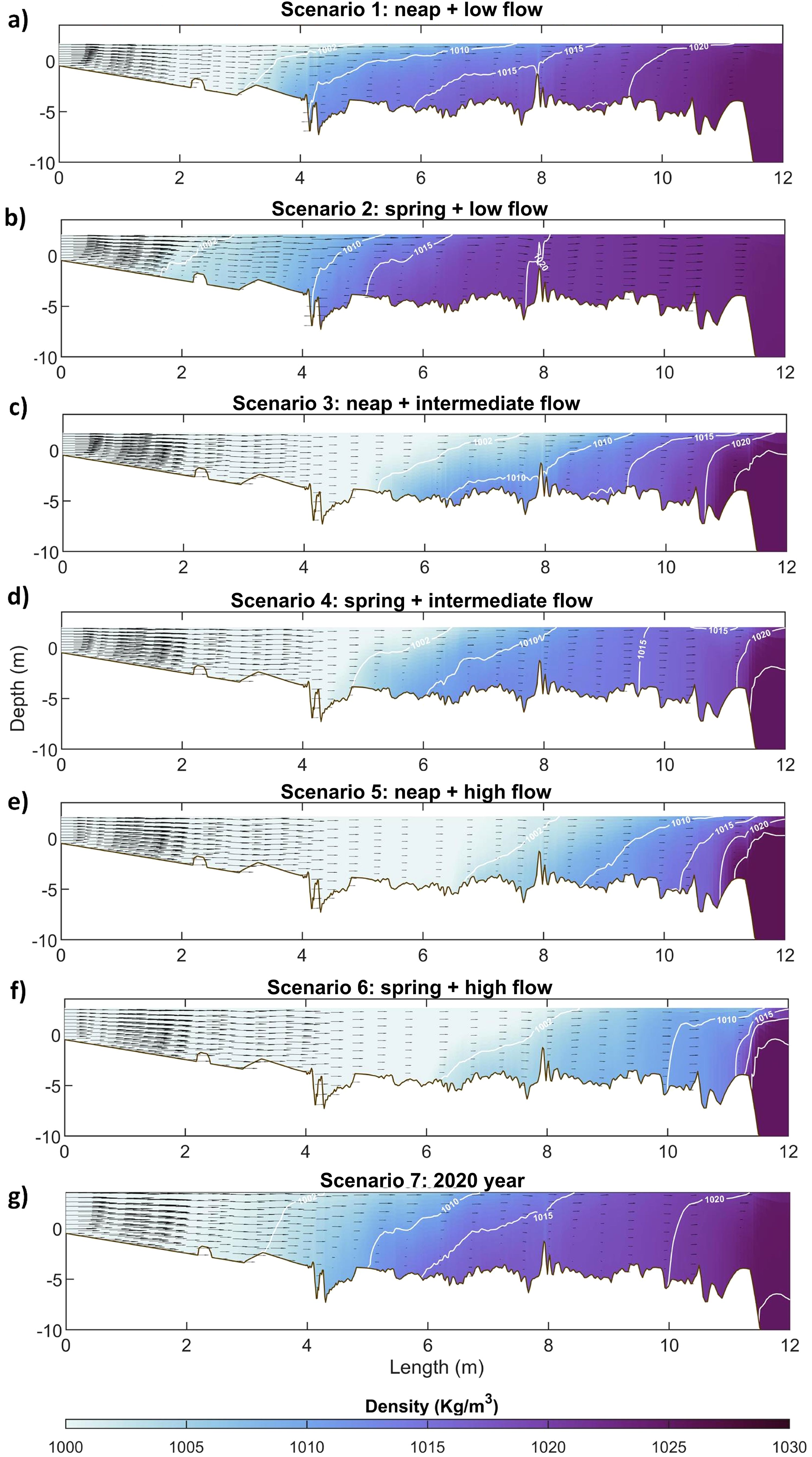
Figure 4. Averaged velocity (black arrows) and density (white lines are the equal density contours of 1002, 1005, 1010, 1015, 1020, and 1025 kg/m³) profiles in section A-A’ for (A) Scenario 1, (B) Scenario 2, (C) Scenario 3, (D) Scenario 4, (E) Scenario 5, (F) Scenario 6, and (G) Scenario 7.

During low flow periods (80% of the 2020 year), the zone with the greatest density gradient is located between kilometers 4 and 8 (33% of the total length of the estuary), while in high flow scenarios, the stratified zone moves towards the mouth, between kilometers 8 and 12 (33% of the total length of the estuary). In these cases, the upper part of the estuary does not show changes in density, as the river invades these areas of the estuary with a homogeneous density. On the other hand, it is noteworthy that, at the mouth of the estuary, the average longitudinal density gradients in section A-A’ are around 30% lower during spring tides than during neap tides. As for the annual situation (Scenario 7) of the estuary, it can be observed a stratification, very similar to that obtained in Scenarios 1 (neap + low flow) and 2 (spring + low flow), as both situations are the most common during the year (80% of the 2020 year).

Next, Figure 5 presents the Hovmöller diagram (Hovmöller, 1949) for ϕ-values during the year 2020. As can be seen in Figure 5, there is a significant influence of river discharge on the location of the stratification zone, as indicated by the black peaks in ϕ that match with the discharge peaks in the upper graph (panel b). During low flows (less than 30 m³/s, 80% of the 2020 year), the zone of greatest stratification, denoted by the yellow color, is located between kilometers 4 and 8 where its maximum value oscillates due to the alternation of spring and neap tides. At neap tides, the stratification is more distributed throughout the estuary during the tidal wave, as river flow reaches 10% of the tidal flow. This distribution only shifts in the different scenarios because of increased flow, reaching up to 35% of the tidal flow at medium river flows and up to 200% at high river flows. However, on spring tides, the stratification zones tend to disappear or reduce in intensity at ebb tide. This is because the spring tide flow doubles the neap tides flow. Due to this stronger outflow of water, mixing of the estuary is favored as one of the main forcing forces is removed.

Figure 5

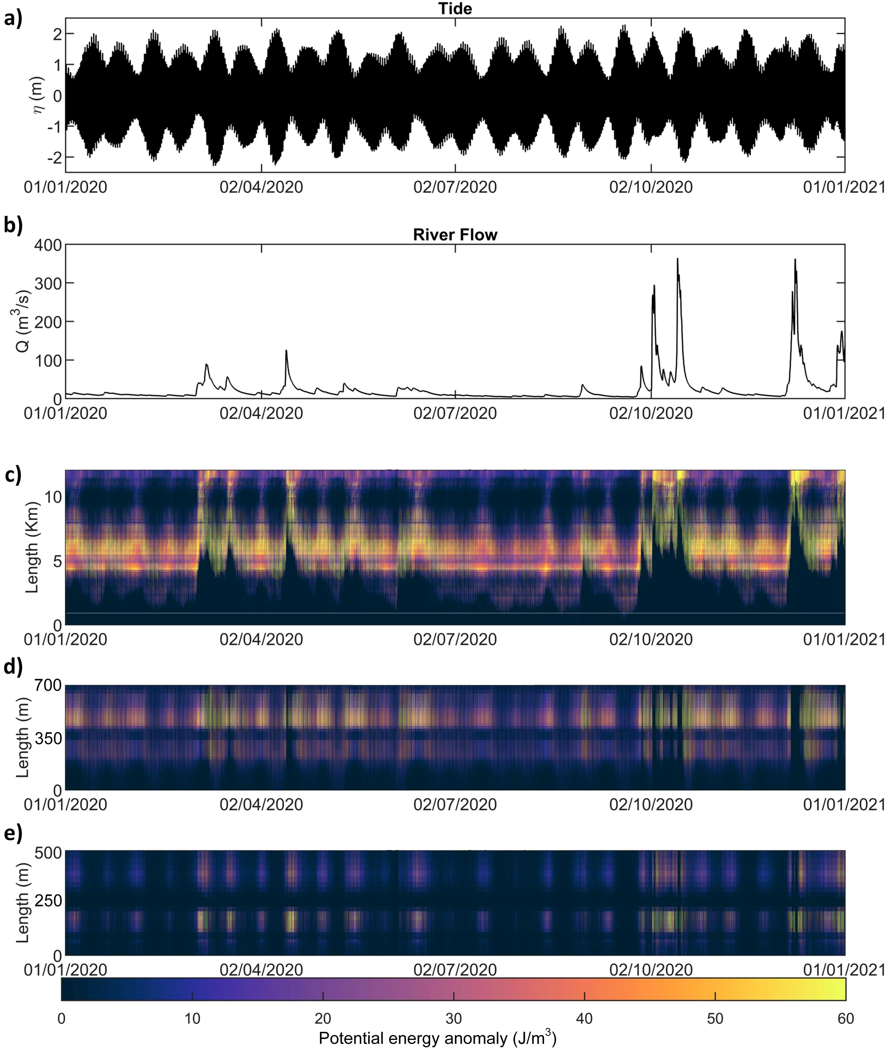
Figure 5. (A) Sea level, (B) River flow and Hovmöller diagram of the year 2020 with hourly ϕ-values along the (C) longitudinal section A-A’, (D) cross section B-B’ and (E) cross section C-C’ (Figure 1). Adapted from Lupiola et al., 2023a.

In the cross sections (Figure 5), the stratification is centered in the main channel, where ϕ picks up the highest values (yellow shadows). Along section B-B’, the river has a significant influence for intermediate flows (30 to 100 m³/s), generating the highest stratification with a value of 50 J/m³ (160% of the annual average ϕ-value in this area). On the other hand, for high flows, section B-B’ is totally mixed, a phenomenon that is not so noticeable along section C-C’. In the C-C’ section, although ϕ values are also higher in the main channel than in the intertidal area (up to 150% higher), the occurrence of a stratification zone is less frequent over time (up to 57% less). It should be noted that, in section C-C’, complete mixing does not occur during high and intermediate flows (values from 2 to 21 J/m³). This is due to its proximity to the estuary mouth since, during these events, the stratification zone is centered in this area as the river flow approaches the tidal flow. However, at low river flows, the whole section C-C’ is mixed due to the tidal effect, as the river flow represents 5% to 10% of the tidal flow. The maximum ϕ-values in this area vary from 10 to 50 J/m³ (60% to 300% of the annual average ϕ-value in this area) depending on the ebb-flood cycle.

At the mouth of the estuary, ϕ-values are very low during spring tides (around 0 J/m³), increasing its magnitude as the tide progresses towards neap tides (up to 20 J/m³, the annual average ϕ-value at the mouth). On the other hand, during high flow events (>100 m³/s, 5% of the 2020 year), the stratification zone moves towards the mouth as the river flow magnitude increases, showing values of up to 200 J/m³ during spring tides, an increase of 1000%. In these cases, areas with very low ϕ-values are observed upstream of the estuary, as all saline water is flushed out by the river discharge.

Figure 6 shows the changes in mixing and stratification in the SE by temporally zooming ϕ in longitudinal section A-A’ (Figure 1) for Scenarios 1 to 6 (Table 1).

Figure 6

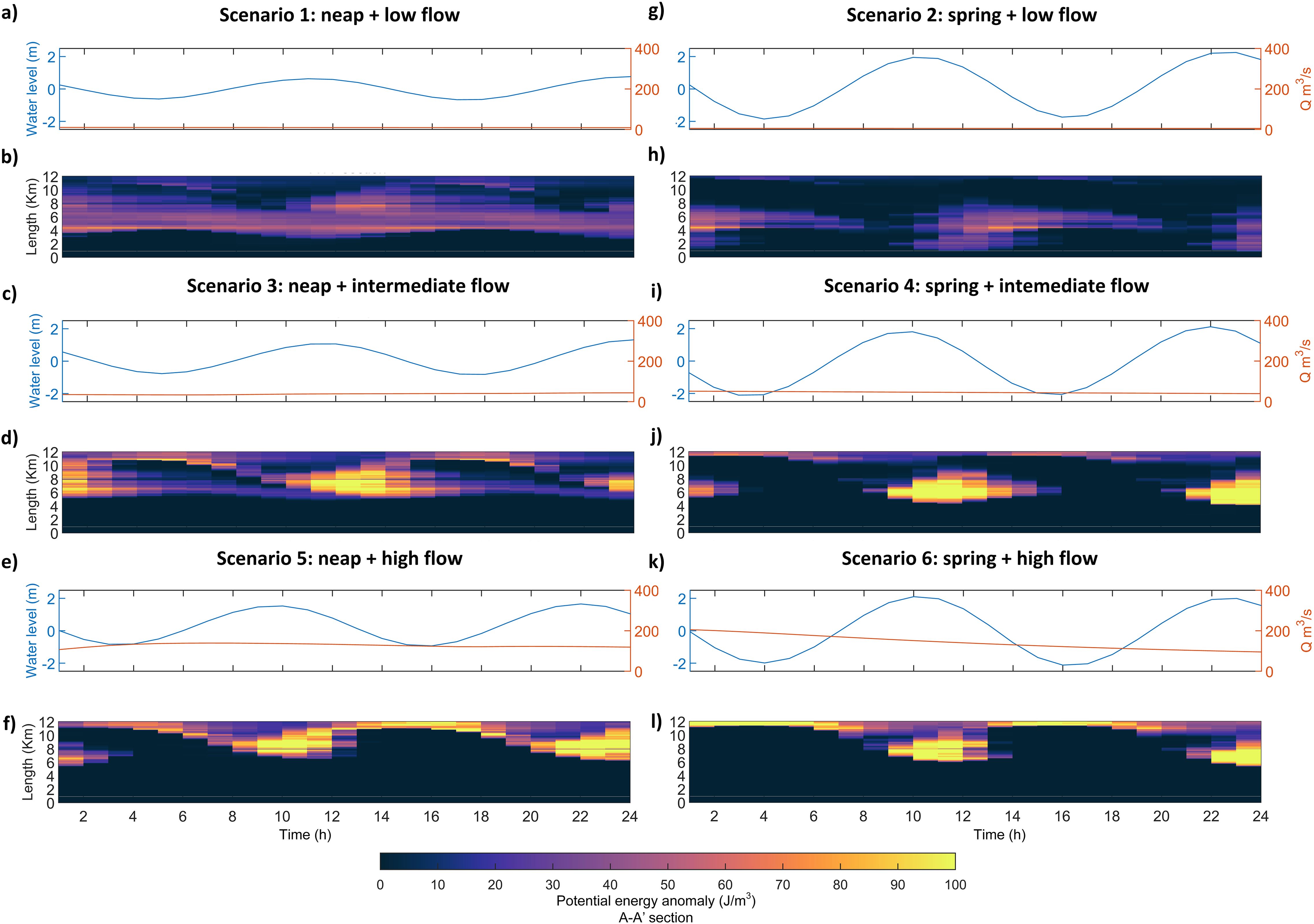
Figure 6. Evolution of flow and tide (A, C, E, G, I, K) and ϕ (B, D, F, H, J, L) at section A-A’ for (A, B) Scenario 1, (C, D) Scenario 2, (E, F) Scenario 3, (G, H) Scenario 4, (I, J) Scenario 5, and (K, L) Scenario 6.

In Scenario 1 (neap + low flow), the stratification zone extends over almost the entire estuary for any tidal phase. At flood tide, the stratification zone starts at kilometer 4 and extends to the mouth of the estuary, which corresponds to approximately kilometer 10 (50% of the length of the estuary). At ebb tide, this zone shifts outwards to approximately kilometer 11, due to the movement of the estuarine waters towards the sea. ϕ-values are homogeneously distributed in the estuary, with the highest values between kilometers 4 and 6 at ebb tide (around 40 to 90 J/m³, 100% and 225% of the mean annual values between kilometers 4 and 6, respectively). At the mouth of the estuary, kilometer 12, the stratification zone has low ϕ-values (equal to annual average ϕ-value, around 20 J/m³), although, throughout the tidal cycle, residual ϕ-values are observed due to the difference in densities between seawater and estuarine water (see Figure 4).

In Scenario 2 (spring + low flow), the stratification zone shifts significantly due to the momentum generated by the spring tide, as the volume of seawater entering the estuary increases (an increase of 200% of the neap tidal flow). During ebb tide, the stratification zone is located, due to the movement of water towards the sea, in the middle zone of the estuary, showing areas with a significant variation of surface and bottom salinity, around 15 kg/m³. Thus, the stratification zone is located between kilometers 2 and 8 (50% of the length of the estuary), reaching ϕ-values of up to 90 J/m³ (250% of the annual average ϕ-value). During tidal flooding, the tidal flow reaches up to 4000% of the river flow. Consequently, a saline front enters and mixes with the estuarine waters for 10 km into the estuary (83% of the length of the estuary). In this situation, ϕ-values are very low or zero as the seawater completely fills the estuary.

In Scenarios 3 (neap + intermediate flow) and 4 (spring + intermediate flow), the stratification zone shifts towards the mouth of the estuary due to river flow, which increases by about 500%, corresponding to 35% of the tidal flow for Scenario 3 (neap + intermediate flow) and 17% for Scenario 4 (spring + intermediate flow). At ebb tide, the stratification zone shifts to the mouth of the estuary due to the combined effect of river flow and tide. Thus, ϕ-values of up to 100 J/m³ occur at kilometer 12 (650% of the annual average ϕ-value at this kilometer). During flood tide, a homogeneous front mixes the estuary with salt water, reaching kilometer 8 (66% of the length of the estuary). During and after flood tide, the highest values are located between kilometers 5 and 10, with ϕ-values above 140 J/m³ (300% of the annual average ϕ-value at this section) due to the combination of tidal (maximum water levels) and river flow.

In Scenario 5 (neap + high flow), high river runoff (between 100 m³/s and 400 m³/s, 5% of the 2020 year) carries estuarine water towards the estuary mouth, flooding the estuary with freshwater, as river flow represents up to 200% of the tidal flow. At ebb tide, a strong river front causes stratification at the mouth of the estuary, between kilometers 10 and 11 (8% of the length of the estuary), with ϕ-values below 100 J/m³. This situation is maintained until the mean level is reached and the tide begins to push the water inland. At this point, the mixing of freshwater and saltwater produces the stratified zone between kilometers 8 and 10 (16% of the length of the estuary), where ϕ reaches values of up to 150 J/m³ (1500% of the annual average ϕ-value at this section).

Finally, in Scenario 6 (spring + high flow), similar effects to those shown in Scenario 5 (neap + high flow) can be observed, although amplified due to the spring tide, as it mobilizes up to 200% more tidal flow than neap tide. At ebb tide, the stratification zone occurs at the mouth of the estuary, as river water almost completely replaces seawater throughout the estuary, creating a marked estuarine-oceanic front. At flood tide, a new front emerges, which moves inland into the estuary and becomes a strongly stratified zone. This stratified zone is located between kilometers 6 and 9 (25% of the length of the estuary), with ϕ-values above 150 J/m³ (500% of the annual average ϕ-value at this section). After flood tide, the stratification zone begins to move towards the mouth of the estuary due to the combined effect of river flow and tide. Once again, the freshwater occupies the entire estuary by a homogeneous seaward displacement front.

3.2 Spatiotemporal evolution of the driving mechanisms of mixing and stratification in Suances estuary

To show the influence of each mechanism, Figure 7 presents the spatial analysis of ϕ using the covariance method during 2020 (Scenario 7), showing: the self-variance of ${\varphi }_t$ (a) and the covariance between ${\varphi }_t$ and (b) S_N, (c) S_M, (d) A_N, (e) A_M, (f) N_N, (g) N_M, (h) C_N, (i) C_M, (j) W_z, (k) Γ, respectively. In this regard, it should be noted that the rest of the terms composing ${\varphi }_t$ have been collected in the term Γ, due to their limited influence on the ${\varphi }_t$-values (Equation 23).

Figure 7

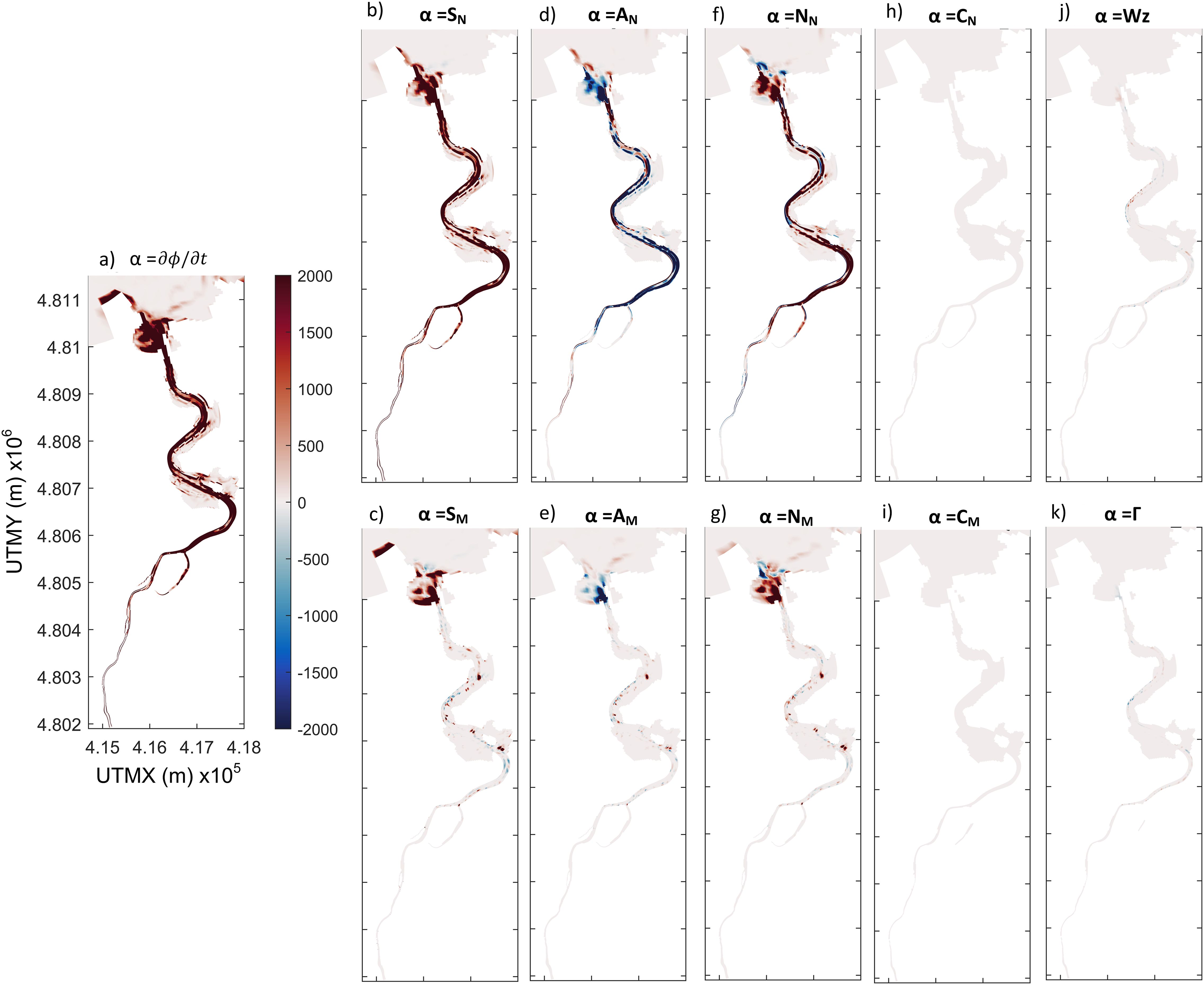
Figure 7. Analysis of the derivative of ϕ (${\varphi }_t$) using the covariance method during 2020 (Scenario 7): (A) Self variance of ${\varphi }_t$ and Covariance between ${\varphi }_t$ and (B) SN, (C) SM, (D) AN, (E) AM, (F) NN, (G) NM, (H) CN, (I) CM, (J) Wz, (K) Γ, respectively.

As can be seen in Figure 7, stratification and mixing, driven by the different mechanisms, is localized along the entire estuary, being of particular relevance between kilometers 4 and 8. Regarding the driving mechanisms in this area, the S_N and N_N mechanisms present the largest positive magnitude (stratification) while the A_N mechanism presents the largest negative one (mixing). In the transverse direction, the effect of S_M and N_M is more significant in the channels entering the intertidal areas, especially in the one located at kilometer 6. On the other hand, from kilometer 11 onwards, the transverse coastal transport processes are observed, where the influence of the terms in the transverse direction becomes relevant. The rest of the mechanisms, such as C_M, C_N, W_z, and those assumed within the term “RESIDUE”, are insignificant and very punctual in certain cells of the model. For this reason, their contribution to the mixing and stratification can be considered negligible with respect to the three main mechanisms (S, A and N; Figure 2). Finally, it is remarkable to note that the main areas of covariance are centered in the main channel, since in the rest of the intertidal areas of the estuary, the values of the mechanisms are much smaller (up to 100 times smaller). Therefore, the most significant changes occur in the main channel.

To analyze the relative strength of each term, the relative contribution of each mechanism is detailed in Supplementary Material 1. As illustrated in Figure 7 and Supplementary Material 1, the S_N mechanism predominates, contributing over 40%. This is followed by the A_N mechanism at 30% and the N_N mechanism at 10%. The combined contribution of all other mechanisms is less than 10% in all cases.

Next, 6 significant points in the estuary have been selected, to analyze the evolution of these mechanisms under the different scenarios defined in Table 1. As shown in Figure 1, these points have been distributed locating three of them in the main channel: downstream of the estuary (point 1), mid-estuary (point 2) and upstream of the estuary (point 3), and the other three points (points 4 to 6) in the intertidal areas. Point 4 has been located next to the WWTP discharge located in intertidal area 1; point 5 in the channel of intertidal area 1 located at kilometer 8; and point 6 in the channel of intertidal area 1 located at kilometer 6.

Figure 8 presents the evolution of points 1 to 3 for the analyzed time periods, i.e., Scenarios 1 to 6 (Table 1), showing on the vertical axes the values of ${\varphi }_t$ and its terms (left axis) whose units are W/m³ and the value of ϕ (right axis) whose units are J/m³. On the horizontal axis, the hours of a tidal wave are shown, coinciding with the first 12 hours of the scenarios shown in Figure 6.

Figure 8

Figure 8. Temporal evolution of the mixing and stratification driving mechanisms, ϕ and ${\varphi }_t$ during a tidal cycle for point 1 (A–F), point 2 (G–L) and point 3 (M–Q) of the scenarios 1 to 6 defined in Table 1. The dotted and the solid lines identify the driving mechanisms in the longitudinal and transversal directions, respectively.

As shown in Figure 8, there is a large variability in the magnitude of the mechanisms depending on the area and scenario analyzed. These values vary from 5 W/m³ (positive and negative) to values of 0 W/m³ because of the total mixing of the water column. At point 1, the S_N and A_N mechanisms take a significant mixing relevance, while N_N tends to compensate for it. However, it can be observed that mixing dominates over stratification in all scenarios except Scenario 5 (neap + high flow), with values even 3 times higher in the negative than in the positive direction. This process takes place from ebb tide, around hour 4, to flood tide, around hour 10, since at this point the entry of a front from the sea pulls a homogeneous front inland. For Scenarios 1 (neap + low flow) and 2 (spring + low flow) (river flow <10 m³/s), the maximum mixing values during the first moments of tidal flooding. In contrast, for Scenarios 3 (neap + intermediate flow), 4 (spring + intermediate flow) and 6 (spring + high flow), the peaks occur as flood tide is reached. This occurs because the increase in river flow (>50 m³/s) causes these mixing processes to be spread out in time, as a greater amount of tidal energy is required to mix the buoyancy provided by the river flow. Finally, in both Scenarios 5 (neap + high flow) and 6 (spring + high flow), an increase in ϕ-values can be observed when high flow (>100 m³/s) and flood tide occur simultaneously. In these cases, the S_N and N_N mechanisms tend to stratify with combined values of up to 5 W/m³, while A_N counteracts these effects with values of up to -4 W/m³.

At point 2, located in the middle part of the estuary between two intertidal areas (around kilometer 7 of section A-A’), differences in functioning can be observed depending on the river flow and tides. At low and medium flows, it is observed that during neap tides, Scenarios 2 (spring + low flow) and 4 (spring + intermediate flow), the N_N mechanism is the main driver mechanism of stratification, whereas for Scenarios 1 (neap + low flow) and 3 (neap + intermediate flow), the N_N mechanism tends to mix. In this sense, the N_N mechanism tends to compensate for the advection acting in the opposite direction, as does the S_N mechanism, except in Scenario 2 (spring + low flow), which tends to stratify. The values of A_N, S_N and N_N are between 0.5 W/m³ and 1 W/m³ for Scenarios 2 (spring + low flow) to 6 (spring + high flow), while for Scenario 1 (neap + low flow) values of 0.1 W/m³ are barely reached. All these changes occur over time until the ebb tide is reached for Scenarios 1 (neap + low flow) to 4 (spring + intermediate flow). During the tidal flooding all driving mechanisms tend towards 0 W/m³. At the same point for Scenarios 5 (neap + high flow) and 6 (spring + high flow), the stratification zone only occurs at flood tide, as the contribution of the high river flow causes this zone to be flooded with freshwater from the river.

Finally, at point 3, located downstream of the estuary, it is observed how during Scenarios 1 (neap + low flow) and 2 (spring + low flow) there is an almost constant stratification along the tidal cycle. For Scenario 1 (neap + low flow), during tidal flushing, the S_N and A_N driving mechanism tend to stratify while N_N tends to mix. On the other hand, A_N tends to mix with tidal flooding while the straining terms (S_N and N_N) decrease their values by about 50%. For Scenarios 3 (neap + intermediate flow) and 4 (spring + intermediate flow), there are variations in the driving mechanisms and ϕ only during flood tide, since in the rest of the tidal cycle the influence of the river shifts the stratification zone downstream. In these situations, the S_N and N_N driving mechanisms tend to stratify while A_N tends to mix. In addition, during spring tides, high values of the three driving mechanisms (S_N, N_N and A_N) are observed, up to 4 W/m³ for Scenario 4 (spring + intermediate flow). These values are a consequence of the confluence at this point of the flood tide and spring tides with the medium fluvial inputs. Finally, for Scenarios 5 (neap + high flow) and 6 (spring + high flow), very low values of the mechanisms are recorded, around 0.001 W/m³. In these situations, the large fluvial contribution makes the entire water column homogenized with freshwater.

Regarding the intertidal areas, Figure 9 shows the analysis of points 4, 5 and 6 located in the estuary as shown in Figure 1.

Figure 9

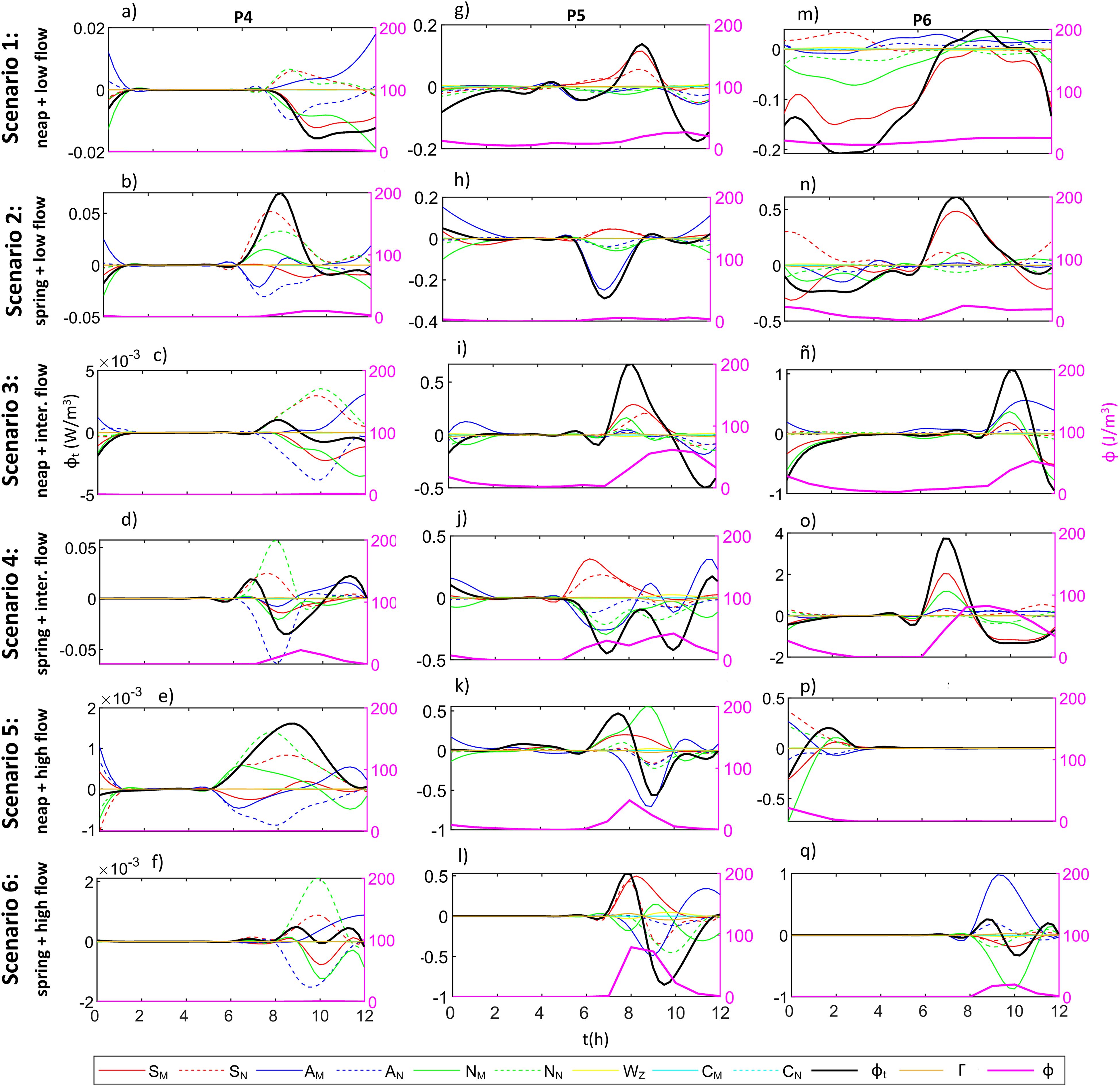
Figure 9. Evolution of the mixing and stratification driving mechanisms, ϕ and ${\varphi }_t$ during a tidal cycle for point 4 (A-F), 5 (G-L) and 6 (M-Q) of the scenarios 1 to 6 defined in Table 1. The dotted and the solid lines identify the driving mechanisms in the longitudinal and transversal directions, respectively.

At point 4, located at an internal point of intertidal area 1 near the discharge of the “Vuelta Ostrera” WWTP, it can be observed that the values of each driving mechanism are in the order of 100 times lower than in the main channel. Furthermore, the values of the driving mechanisms are zero during all phases of the tide except at flood tide, when salt water is introduced into the area where point 4 is located. In these situations, stratification occurs, led by the S_N and N_N driving mechanisms, which is balanced by the mixing produced by the A_N driving mechanism. The influence of the longitudinal direction occurs because the flooding of these intertidal areas occurs because of the tide advancing longitudinally in the estuary. During the flushing of the tide, the A_M driving mechanism stratifies the water column while the S_M and N_M mix it, because of the transverse flows caused by the WWTP discharge, which has a flow rate between 10% and 20% of the river flow in low flow scenarios.

At point 5, the values of the driving mechanisms increase significantly to values of 0.5 W/m³. This point 5 is located at one of the tidal creeks of the intertidal area, so the influence of transverse processes is especially significant, governing the competition between mixing and stratification in the area. The greatest changes in stratification occur during tidal flooding since the water flow enters in a transverse direction. Thus, the S_M driving mechanism is the predominant stratifying, while the A_M driving mechanism tends to compensate for it.

Finally, the influence of the driving mechanisms at point 6 has been analyzed, which is in the tidal creek of the intertidal areas upstream of the estuary (kilometer 6). At this point, cross-directional driving mechanisms predominate in mixing and stratification. In addition, there is a tidal influence for all scenarios, increasing stratification at flood tide. In Scenario 4 (spring + intermediate flow) a large stratification occurs when the intertidal area begins to flood, introducing a large amount of water of different density in the transverse direction. This originates values of up to 4 W/m³, led by the S_M and N_M driving mechanisms.

3.3 Final zoning of the driving mechanisms of mixing and stratification in Suances estuary

Figure 10 compiles 9 spatial distributions maps showing the final zonation of the mixing and stratification driving mechanisms in the SE indicating: (a) the most probable positive mechanism (stratifier), (b) the most probable negative mechanism (mixer), (c) the most probable absolute driving mechanism, (d) and (g) persistence and maximum persistence time of the positive mechanism (stratifier); (e) and (h) persistence and maximum persistence time of the negative mechanism (mixer) and; (f) and (i) persistence and maximum persistence time of the absolute mechanism for the simulated 2020 year.

Figure 10

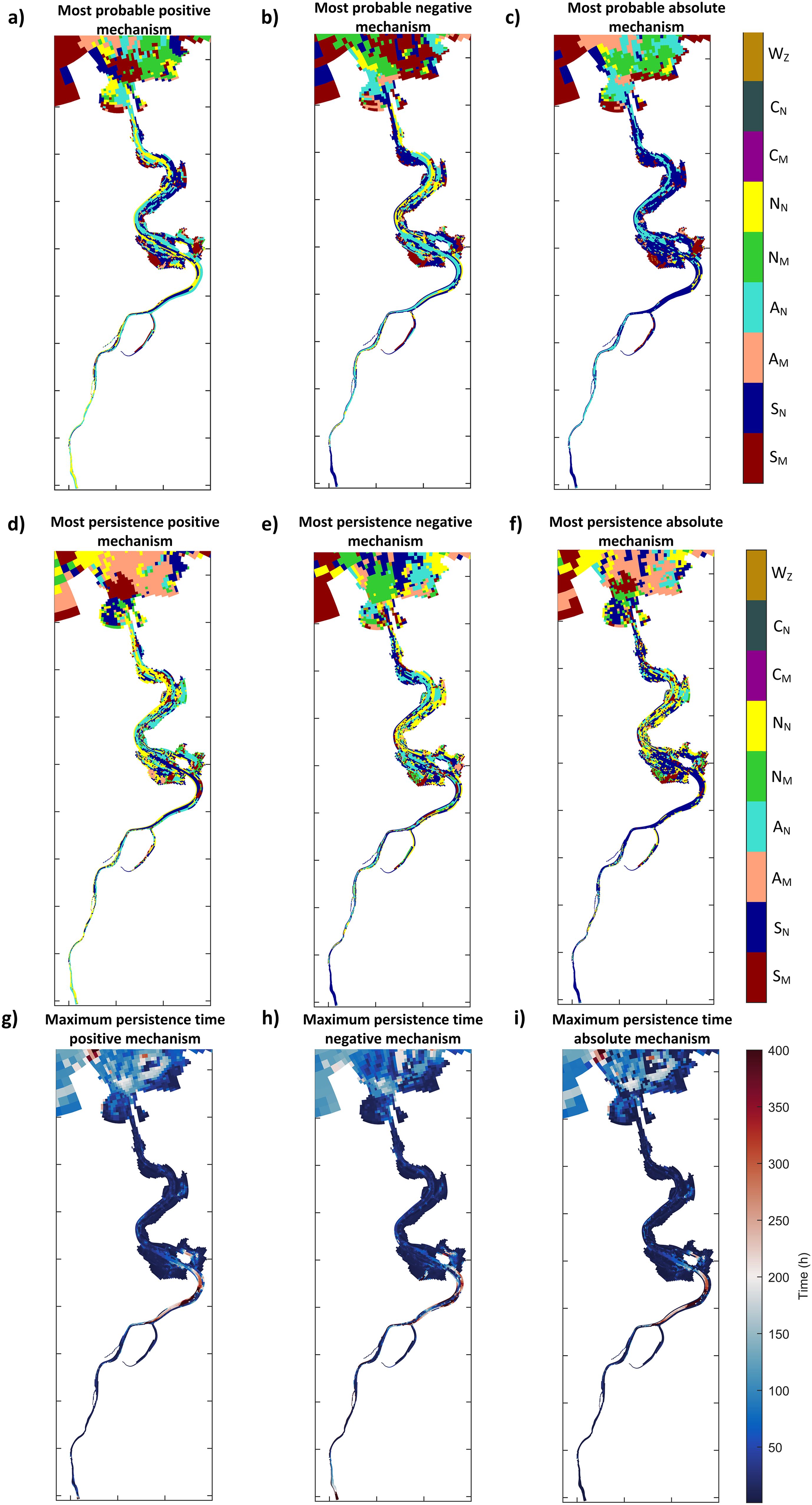
Figure 10. Final zonation of mixing and stratification driving mechanisms in Suances estuary: (A) most probable positive mechanism (stratifier), (B) most probable negative driving mechanism (mixer), and (C) most probable absolute mechanism (D, G) persistence and maximum persistence time of the positive mechanism (stratifier); (E, H) persistence and maximum persistence time of the negative mechanism (mixer) and; (F, I) persistence and maximum persistence time of the absolute mechanism.

As shown in Figure 10, the S_N driving mechanism presents a significant predominance in the SE, followed by the A_N driving mechanism, as observed in panel c) of Figure 10. Mainly, the S_N driving mechanism predominates in a positive sense (stratifying) around the channel where the confluence between the fluvial and tidal water masses occurs, between kilometers 4 and 8, coinciding with the maximum ϕ-values in low/medium flow situations. However, in the rest of the main channel, there is a predominance of the A_N driving mechanism in the positive direction. In the intertidal areas, the S driving mechanism, both longitudinally and transversely, becomes relevant in the positive direction, depending its magnitude on the predominant direction of flow. As for the negative compensators (mixers), it can be observed that both S_N and A_N tend to compensate each other. However, the compensating driving mechanism that is most often repeated throughout the estuary is N_N, as can be seen in panels a) and b) of Figure 10. At the mouth of the estuary and the adjacent coast, the transverse direction becomes more relevant, with the S_M and N_M driving mechanisms being the drivers of mixing and stratification.

The driving mechanism of maximum persistence is S_N in the positive direction (stratifier) and A_N in the negative direction (mixer), from kilometer 0 to 7 of the estuary. In addition, it is possible to observe how in the inner parts of the curves a higher persistence is obtained, registering values of up to 300 hours with a tendency to stratify. From kilometer 7 to the mouth of the estuary (kilometer 12), the influence of the S_N, A_N and N_N driving mechanisms is distributed as a mosaic along the estuary in both positive and negative directions. The persistence in this zone is less than 50 hours, presenting a greater variability than that obtained for the most probable driving mechanism. On the other hand, it should be noted that, in the inner part of the “Vuelta Ostrera” curve, the S_M driving mechanism drives the mixing, with a persistence of around 100 hours, due to the secondary circulation that occurs in this area.

Another remarkable process is the effect generated by the WWTP discharge on mixing and stratification in the intertidal area. In this regard, it is important to note that the WWTP continuously discharges freshwater in the transverse direction, causing the S_M term to drive the mixing of the water column while the A_M driving mechanism drives the stratification of the column with persistence times of up to 100 hours in the form of stratification. Therefore, the intertidal area is locally stratified due to the introduction of a higher buoyancy (freshwater) flow into the system than the saltwater entering from the main channel, whose contribution to stratification cannot be compensated by the turbulence generated by bottom friction.

4 Discussion

4.1 Influence of forcings on mixing and stratification

Mixing and stratification processes in an estuary are determined by the characteristics of water circulation, which, consequently, depend on the conditions of forcings, geometry and estuarine bathymetry. For this reason, spatial changes in stratification can be found instantaneously (Valle-Levinson, 2021). In the SE, the levees bordering the main channel (more than 13000 m) and the jetty located at the mouth constrain the flow laterally before reaching the ocean, forcing the water to flow through a small cross section as it moves towards the coast. Current urban civil developments produce larger currents than would be present without human intervention, influencing vertical mixing (Arévalo et al., 2022). In addition, the intertidal areas are connected to the main channel by secondary channels between the levees, which causes these areas to flood and flush at different times with respect to the main channel, causing the stratification that occurs in the intertidal areas to be much less than that of the main channel. However, when river floods occur, these levees are overtopped, which tends to homogenize the cross sections and promote stratification in the intertidal areas similar to that of the main channel.

In the SE, as in other small estuaries, the regulation of mixing and stratification is actively dynamic along its entire length (Figure 4), with more intensity at certain locations and different times, depending mainly on the tide, which determines its spatial variation as a function of the tidal phase (ebb-flood tidal cycle). Moreover, the regulation of mixing is strongly modulated in time by the spring-neap tide cycle, as also described by MacCready et al. (2018). Azhikodan et al. (2021) noted that, in the Tanintharyi River estuary, this phenomenon can be attributed to the strong dominance of tidal flow over fluvial flow. In SE, during the year 2020, 80% of the time the tidal flow was 2000% higher than river flow in low river flow scenarios. However, when a river flood occurs (an increase up to 3000% of the river flow), these extraordinary freshwater inputs carry the stratification zone towards the mouth of the estuary. Depending on the magnitude of the fluvial input, the stratification zone moves further outward and may even displace all the saline water in the estuary towards the sea if, at the same time, fluvial flood events occur with ebb tides (Figure 5). This behavior has been reported recently in other estuaries by Zachopoulos et al. (2020); Otero et al. (2021); Wang et al. (2022), and McKeon et al. (2021). Such a phenomenon can be attributed to the dominance of fluvial flow during flood events (5% of the time with high flows greater than 100 m³/s, where the river flow can double the tidal flow), because the geometry of the SE (small estuary) is highly sensitive to the volume of water introduced into the system. As pointed in Bárcena et al., 2012b, the flushing time in SE varies from 2 days in low flow and ebb time conditions to 9.6 hours in medium flow, showing the high variability of the SE. Therefore, as shown by Xiao et al. (2020) in the Sydney estuary, variations in intra and intertidal vertical mixing highlight that, rather than being in a tidally averaged steady state, the estuary is in a continuous state of adjustment to variations of its forcing conditions.

Spatially, the area between kilometers 4 and 8 (33% of the length of the estuary) shows the greatest stratification due to the influence of the tides, which, depending on the phase of the tide (ebb tide or flood tide), advances or retreats promoting the stratification and mixing respectively. Variations are also observed due to spring and neap tide cycles. During neap tides, ϕ-values are usually more localized in the estuary since, in these situations, the tide produces a greater inflow (flooding the estuary) and outflow (flushing the estuary) of water while, during neap tides, the meeting zone between the two water masses is more distributed throughout the estuary. During river flood events, this zone is modified starting at approximately kilometer 6 and extending to kilometer 10 or even outside the mouth of the estuary, covering up to 50% of the length of the estuary.

These findings align with the results obtained by Garcia and Geyer (2023) in an idealized numerical model based on the North River, which examined the migration of the convergence front in response to changes in the tidal regime (ranging from daily to monthly). Additionally, a threshold has been identified between ϕ-values and the depth of the water column. As shown in Equation 1, ϕ is defined by the integration of density over depth, making depth a fundamental parameter. Since ϕ represents the energy required to homogenize the water column, it is expected that this energy will increase with depth, especially in scenarios with identical density gradients. However, for varying density gradients, depth also plays a significant role, as deeper estuaries will consistently exhibit higher Potential Energy Anomaly (PEA) values due to the increased influence of depth on these values. This relationship is reflected in Equation 1, where the integration of density fluctuation with depth results in a multiplicative effect, meaning that greater depth leads to higher ϕ values. Figure 11 illustrates the average ϕ-value in the SE for Scenario 7 (the full year 2020), highlighting the threshold between depth and ϕ-values for both the main channel and intertidal areas.

Figure 11

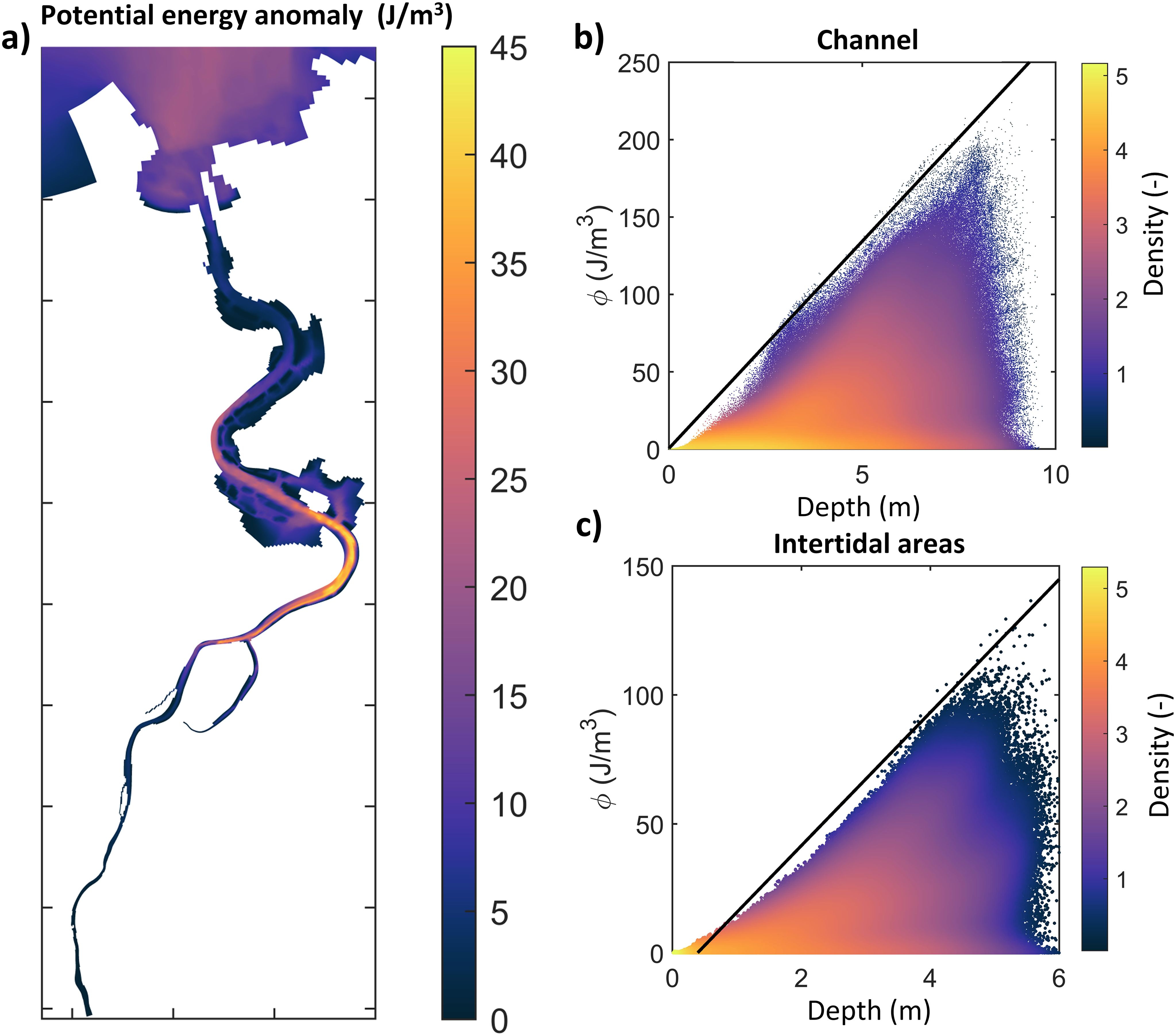
Figure 11. (A) Mean ϕ value in Scenario 7. Density plot correlating ϕ-values with depth for: (B) the main channel and (C) intertidal areas. Black line represents a linear regression for the simulate time range of the upper bound of the values of the ratio of the AEP and H.

As mentioned above, there is a zone of maximum stratification between kilometers 4 and 8, reaching average ϕ-values of up to 45 J/m³, which are located in the main channel and in the channels connecting the intertidal areas. On the other hand, it can be observed, in panels b and c of Figure 11, how the most usual of ϕ-values are close to 0, because the estuary is not stratified most of the time throughout the year.

Interestingly, within the simulated time range, depth clearly limits the maximum ϕ-values, showing a practically linear upper limit for both the main channel and the intertidal areas. It is important to note that this limit is an approximation of the phenomenon indicated by the upper average limit, which can be modified by introducing more simulated data or altering the bathymetric, geomorphologic, or boundary conditions of the estuary. The highest ϕ-values, reaching up to 200 J/m³, occur only in high flow scenarios combined with spring tides (5% of the time in 2020). In these situations, the depth and density are at their maximum, generating the highest stratification values. Conversely, during low flow events (80% of the time in 2020), ϕ-values barely exceed 40 J/m³ in the areas of greatest stratification because a smaller water column and lower density gradient require less energy to homogenize the water column.

Based on these results, it can be established that ϕ is highly sensitive to depth. Therefore, ϕ-values cannot be directly compared with those of other estuaries with greater depths. Alternative classifications must be sought to compare estuarine systems with each other, as demonstrated by Lupiola et al. (2023b).

4.2 Spatiotemporal changes in mixing and stratification

Depending on the magnitudes of the forcings in the estuary, the prevalence of mixing and stratification driving mechanisms will change in each zone of the estuary because of the interaction of the confluent water masses. The regimes may also change over time (e.g., seasonal cycle, neap-spring tide cycle, flood-ebb tide cycle) and, therefore, also the equilibrium of the potential energy anomaly and their derivative terms (Burchard and Hofmeister, 2008). Furthermore, depending on geometric and bathymetric characteristics, there are spatially differentiated zones within an estuary (Bárcena et al., 2012b) which, in turn, modify the driving mechanisms in different zones of the estuary for the same forcings.

The SE can be divided into a main channel, which can be subdivided into three zones that vary spatially and temporally depending on the tides and fluvial inputs: main channel, intertidal areas and the mouth of the estuary. In each of these zones, certain mechanisms will predominate and favor mixing and stratification depending on the forcings. Within the main channel, a first zone can be found upstream of the estuary, in the most inland zone, where the fluvial water prevails. After this zone, a confluence zone will be found, which will be the meeting point of the fluvial and tidal waters. Finally, from this confluence zone to the mouth of the estuary, there will be a zone where the tide will be predominant. Along with these three zones, intertidal areas can also be found, where different processes occur due to changes in geometry and currents.

Figure 12 presents a sketch of the main mixing and stratification driving mechanisms that are most likely to occur in the SE. Upstream of the estuary, the influence of the river is the main forcing. In this part of the estuary, the piston effect created by the advective force of the river (A_N driving mechanism) prevails in the mixing, since it drives a practically homogeneous density profile (fluvial input) towards the sea. However, in the initial zone, from kilometer 0 to 1, it should be noted that the S_N driving mechanism predominates in the mixing. This occurs because in this zone there is only fresh water coming from the river, since the tidal intrusion does not reach these zones. The A_N driving mechanism is influenced by density fluctuations, and these are zero (Figure 4) in this section so, the velocity fluctuations make up the S_N driving mechanism predominate. As mentioned above, outside this first kilometer, the driving mechanism for mixing is the A_N driving mechanism, with values up to 100 times higher than the S_N and N_N stratifying counterparts, due to the piston effect produced by the river displacing the homogeneous fluvial front.

Figure 12

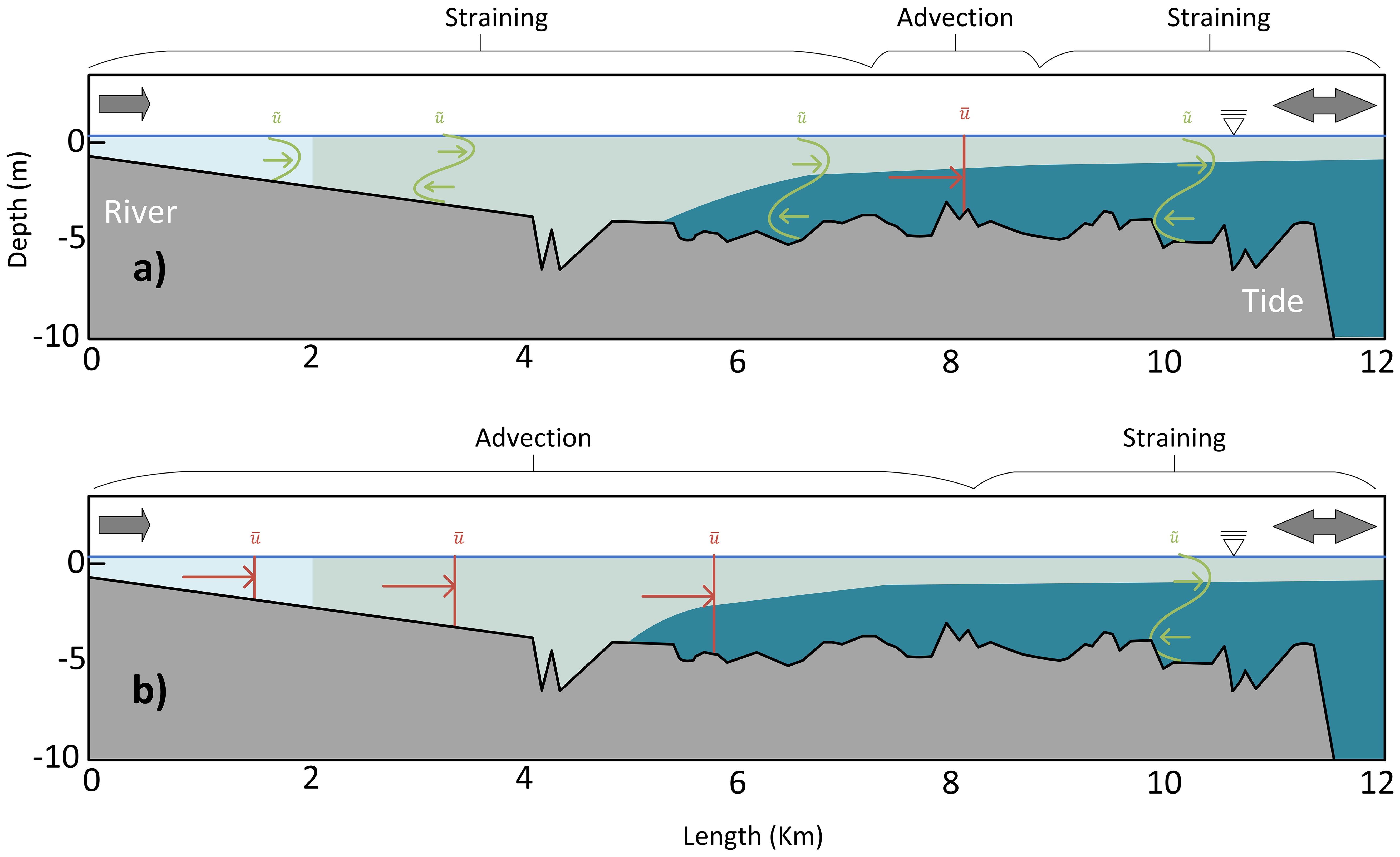
Figure 12. Conceptual model of the mechanisms driving the processes of (A) stratification and (B) mixing in Suances estuary in section A-A’.

After the fluvial influence zone, which has a practically homogeneous behavior in all scenarios, the stratification zone of the estuary is located. This zone is most probably situated between kilometers 4 and 8, where the confluence of fresh and salt water occurs most of the time (Figure 11). This zone is the most active in the stratification processes, since mixing does not occur only longitudinally, also the surrounding bends and intertidal areas favor transverse flows and zones of secondary circulation. In this area, variable behavior can be found according to the flood and ebb tide cycles, as well as the neap and spring tide cycles. Finally, in the section located from kilometer 8 onwards, it can be seen how the S_N straining term predominates.

Figure 13 presents a conceptual scheme of the estuarine circulations. As illustrated, stratification primarily depends on fluvial and tidal inputs in the longitudinal direction, which generate the main mixing and stratification patterns. However, secondary mixing processes (Bo and Ralston, 2022) can also contribute to mixing and stratification. In the SE, secondary mixing is not a significant factor except in specific areas such as sharp bends (Becherer et al., 2015; Geyer et al., 2020), constrictions (Geyer et al., 2017), and intertidal channels.

Figure 13

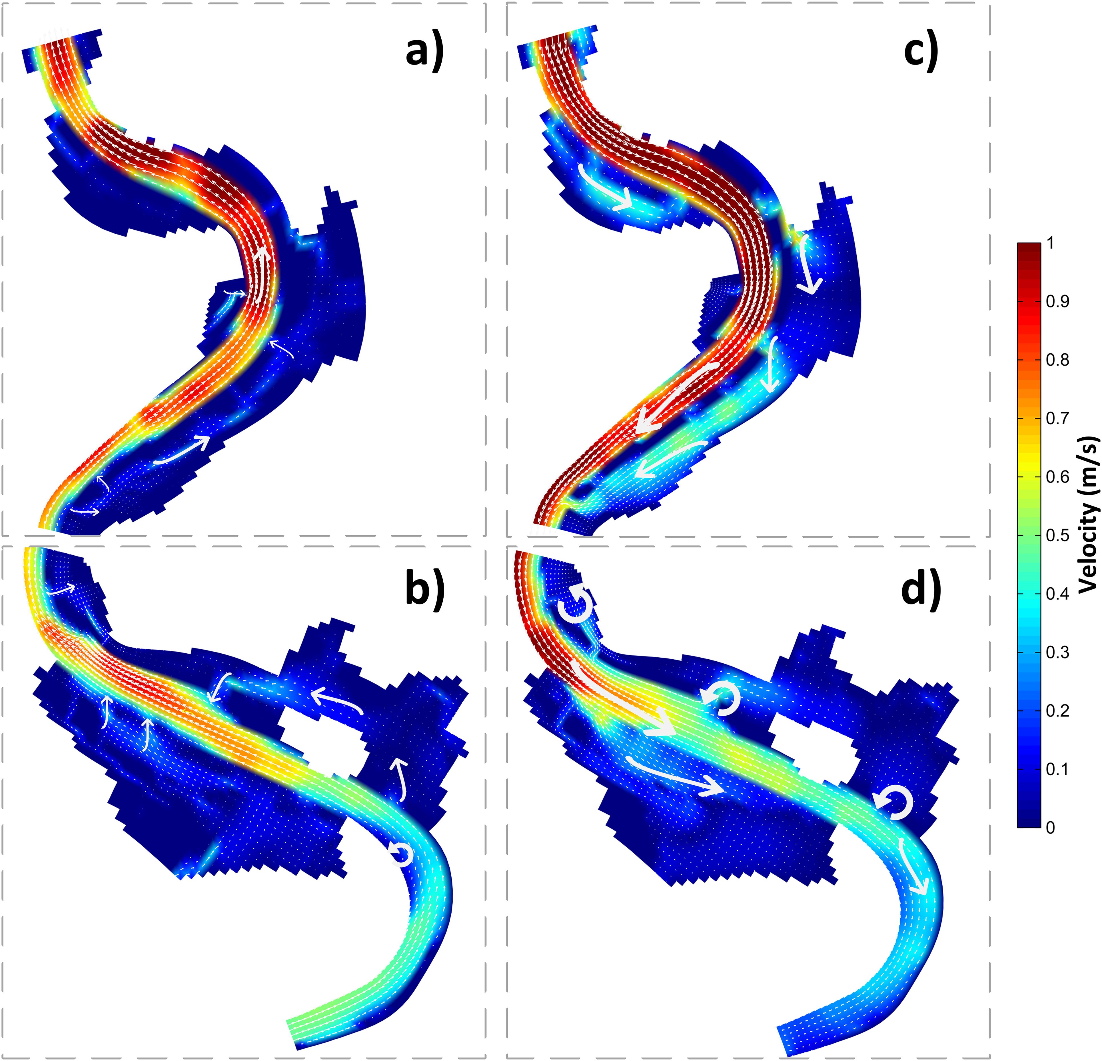
Figure 13. Conceptual scheme of Suances estuary during ebb tide (A, B) and flood tide (C, D), where the velocity field and circulation flows are shown with white arrows. The details shown in these figures correspond to panels b and c of Figure 1.

During the tide flushing, a process of flow separation or recirculation occurs at the “Vuelta Ostrera” curve, located at kilometer 6. This flow separation is a result of the location in these areas of sediment deposits raised approximately 2 m above the main channel, which causes the water recirculation and, therefore, the water mixing in this area. For this reason, in Figure 11, it can be appreciated that in this inner zone of the curve the average ϕ-values are lower compared to the main channel (approximately 20%) because this zone favors the mixing of the waters, making the stratification disappear. This behavior has been reported in other studies (Bo and Ralston, 2022), where it has been concluded that these closed curves favor the appearance of dead flow or flow separation zones.

In “Vuelta Ostrera” curve, the S_N driving mechanism tends to mix while N_N tends to stratify by the recirculation of the flow, with A_N not intervening since, at this point, the velocities are very low or almost zero.

Figure 14 presents two schemes (with flood and ebb tides) during spring tides in cross sections B-B’ (panels a and b) and C-C’ (panels c and d) of Figure 1. In this figure, the velocity fields as well as the density contour lines, and density values are shown. Additionally, white arrows show a conceptual scheme of the directions of the velocity vectors during the flooding, panels a and c, and during the flushing, panels b and d.

Figure 14

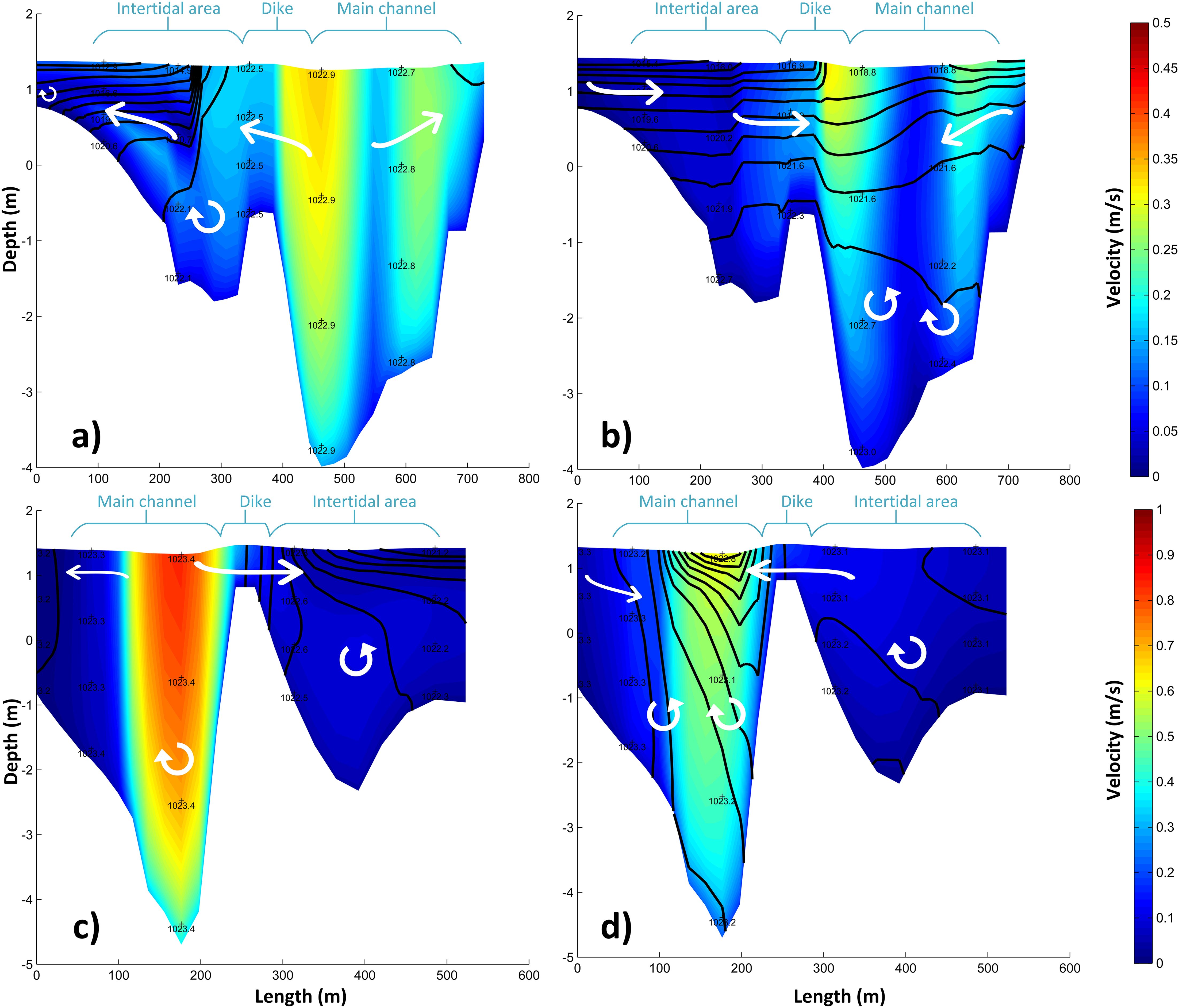
Figure 14. Conceptual scheme of Suances estuary during tidal flooding (A, C) and flushing (B, D), where the velocity field and transverse velocity vectors are shown schematically with white arrows. In addition, the density contour lines, and their values are included. These sections correspond to section B-B’ (A, B) and section C-C’ (C, D) of Figure 1.

As shown in panels c and d of Figure 14, the secondary circulation is observed in the curves. However, as the longitudinal flows in the estuary dominate, this effect hardly affects the mixing of the water column, since the velocities occurring in the transverse direction are 5 to 10 times lower than in the longitudinal direction. For this reason, the mixing effect produced by this process is reduced by the longitudinal stratifying effect of the confluence of fluvial and marine waters. In these cases, it is possible to find the mechanisms in the transverse direction favoring mixing, although their contributions are in the order of 10 times less than in the longitudinal direction.

Another aspect, which can be seen in Figure 13 and Figure 14, is the cross flows that occur because of a migration of water from the main channel to the intertidal areas and vice versa. During tidal flooding, the denser seawater flowing through the main channel floods the intertidal areas through the tidal creeks, while as the tide recedes (flushing), the intertidal areas tend to drain, displacing the denser water from the intertidal areas into the channel. As these areas are separated from the main channel, the process of flooding and flushing occurs in a time-delayed pattern, functioning as dead zones or “traps”. At flood tide, these slower flow regions remain relatively fresher than the faster flowing regions of the channel and, at ebb tide, they remain relatively saltier. These lateral density gradients combined with the steady flow in the intertidal area drive a baroclinic circulation that increases stratification in the intertidal areas in a transverse direction (Garcia and Geyer, 2023), as seen in Figure 14.

In addition, these inflows/outflows of water through the tidal creeks into the intertidal areas have a direct influence on the main channel, which is reflected by the increased importance of the N_N driving mechanism. During spring tides, the contributions of these waters from the intertidal areas in the transverse direction favor the negative growth of the N_N driving mechanism. The reason for this growth can be found in the inclusion of a large amount of water of different density that favors mixing, which is compensated, in the positive direction (stratifying), by the A_N driving mechanism, because of these stratified waters are displaced by the effect of advection towards the tidal creek.

However, during neap tides, the contribution from the intertidal areas is smaller and, therefore, promotes the growth of nonlinear straining (N_N) stratifying. In this case, as velocities in the tidal flushing are found to be lower than in the spring tide, A_N tends to compensate for this stratification. This fact is reflected in the water circulation, where it can be observed that the filling of intertidal areas by fluvial water only occurs during spring tides, when the tide recedes sufficiently to facilitate the entry of fluvial water to flood that volume.

As far as the main channel is concerned, the intermediate zone (kilometers 4 to 8) has the largest stratification zones with the highest ϕ-values (Figure 11). In this zone, the main mechanism driving the stratification is the S_N, due to the shear effect produced by velocity fluctuations at the confluence of two water masses: the tidal entering from the bottom and the river flowing through the surface. In these cases, the main driving mechanism that attempts to compensate for this stratifying effect is the A_N driving mechanism, pushing the semi-homogeneous fronts. However, this is not sufficiently strong since, in this zone, the velocity fluctuations are very high and in opposite directions in the vertical profile. As a result, the greatest stratification occurs and, therefore, the highest ϕ-values.

From kilometer 7 to exit of the estuary there is a constriction of the main channel (Figure 13) due to the construction of artificial dikes that separate the intertidal areas. Due to these constrictions, the recirculation effects that have been observed in the “Vuelta Ostrera” curve (kilometer 6) disappear, since the inflow and outflow velocities are higher, and can be as much as double (Figure 14). In this area, especially in the curve at kilometer 8, there is a significant increase in speed, which causes the flow to accelerate. Consequently, Figure 10 shows how the A_N driving mechanism favors stratification, since it displaces the stratified fronts with little deformation. Outside this curved zone, tidal straining processes, especially nonlinear (N_N) because of water inputs from intertidal areas, have a predominance in stratification, while A_N predominates in mixing (Figure 12).

Finally, in the adjacent coastal zone, from kilometer 12 onwards, the processes are significantly modified. In this zone, the transverse direction takes on a greater influence, originated by the transverse currents that occur on the coast, and the expansion of the outflow of water from the estuary constrained by the levees towards the open sea, expanding in all directions.

Regarding the intertidal areas, it can be observed how in the areas farthest from the main channel, the driving mechanisms in the transverse direction have a greater influence, originated by the lateral flows (Figure 10). Another singular zone are the tidal creeks that link these intertidal areas with the main channel since strong velocity gradients occur at these locations during flooding and flushing. At these points, where inflow and outflow occur in a single direction (Figure 14), the S_M and A_M driving mechanisms are predominant in mixing and stratification, respectively, as can be seen in Figure 10. These lateral flows, which are introduced into the main channel with different salinity, favor the influence of N_N, because one of the key factors in determining its importance is the contributions of the discharge of the tidal creeks on the main channel. Another noteworthy point, within the intertidal areas is the continuous freshwater discharge from the WWTP, where the A_M driving mechanism is the predominant mechanism as can be seen in Figure 10. At this point, there is a continuous inflow of water in a transverse direction, which makes the advection in a transverse direction predominant.

Due to the sensitivity of small estuaries to the volume of water introduced into the system, as is the case of the SE, mixing between two differentiated water masses occurs rapidly, causing the mixing and stratification zone to be highly influenced in position and intensity by external tidal and river forcing. In this way, velocity and density fluctuations are produced causing stratification through the different mechanisms analyzed. Because of this rapid and spatiotemporally variable mixing, the S, A and N driving mechanisms become the main drivers of mixing and stratification, since they are directly influenced by these velocity and density fluctuations caused by Reynolds decomposition. Furthermore, because of this sensitivity to the volume of water introduced, density gradients can be found where, for a shallow depth (3 to 8 m), all seawater is located at the bottom and river water at the surface. This water distribution coupled with velocities of around 1.5-2 m/s allows the development of mechanism values which are much higher (even 100 times higher) than in other estuaries or coastal areas with higher water volumes (de Boer et al., 2008; Wang et al., 2022; Zhang et al., 2023).

Regarding the influence of each driving mechanism, de Boer et al. (2008) identified the S and A mechanisms as the primary drivers in coastal areas. However, studies by Wang et al. (2022) and Zhang et al. (2023) on two tidal creeks of the Changjiang estuary revealed that in the northern channel, which features levees, flow-constricting elements, and intertidal areas, the N driving mechanism’s values increased (Wang et al., 2022). Conversely, in channels without such elements, the N driving mechanism became a residual mechanism compared to the S mechanism (Zhang et al., 2023). Although the SE is not a small estuary, similar behavior is observed regarding the impact of anthropogenic structures on the main channel.

In the SE, the observed results reflect a combination of anthropogenic effects and the estuary’s small size. For instance, areas of estuarine constriction and consequent flow acceleration are primarily due to the natural characteristics of the estuary, which have been exacerbated by anthropogenic actions such as the construction of dikes. It is evident that these structures significantly impact intertidal channels by inducing cross flows, which create mixing and stratification zones. These non-linear deformations enhance their influence, a phenomenon that would not occur in the absence of these structures.

Anthropogenic structures thus play a crucial role in modifying the hydrodynamic behavior of the estuary. They not only alter the natural flow patterns but also contribute to the formation of distinct mixing and stratification zones. This highlights the importance of considering both natural and human-induced factors when studying estuarine dynamics, as the interplay between these elements can significantly affect the overall hydrodynamic and ecological characteristics of the estuary.

Therefore, in estuarine systems that present a main channel, in which the flow is constrained by dikes and intertidal areas, the nonlinear straining driving mechanism (N) has a significant relevance since, despite not being the predominant one, it has a presence in all the mixing and stratification zones as a secondary driving mechanism in accordance with the nonlinear phenomena that occur in these turbulent zones. This phenomenon can be amplified in small estuaries, since they do not need to have elements or dikes to constrict the flow because their own geometry tends to create these intertidal areas, giving rise to a similar effect.

Finally, it is important to emphasize that this study did not account for the morphological evolution of the estuary. Changes in sediment input or withdrawal could modify the estuarine bathymetry and, consequently, alter the mixing and stratification patterns observed. Additionally, the accuracy of this study and numerical model is higher in the main channel, while the adjacent coastal and intertidal areas are approximations that should be interpreted with caution. Future studies should focus on providing a more precise detailing of the intertidal areas, integrating them with the main channel to enhance the overall accuracy of the model.

5 Conclusions

The mechanisms controlling mixing and transport vary in time and space due to complex interactions between hydrodynamic forcings (tidal and fluvial discharge) and geomorphology (bathymetry and geometry). The applied methodology in a 3D numerical model for understanding estuarine features and the driving mechanisms of mixing and stratification could help researchers, technicians and/or policy makers to manage them more efficiently.

The use of the potential energy anomaly (ϕ) as a parameter to measure stratification: (1) allows quantifying the magnitude of the stratification (in this study from 0 to 200 J/m³), (2) offers the possibility of analyzing its evolution in time by temperature and salinity modifications, and (3) facilitates its application to three-dimensional models since it only depends on the knowledge of the density field in the water column.

Following the work carried out on the Suances estuary by Lupiola et al., 2023a, the numerical results show that Suances estuary presents a high variability of mixing and stratification driven, firstly, by river flow (seasonal cycle - monthly time scale), secondly, by tidal phase (flood-ebb tide cycle - diurnal time scale) and, finally, by tidal magnitude (neap-spring tide cycle - fortnightly time scale). Furthermore, these results explicitly highlight how the driving mechanisms can vary for the same estuarine geometry at different locations due to diurnal, fortnightly and seasonal changes in forcing.

On the other hand, a threshold was found between the potential energy anomaly and the depth of the water column, confirming that there are limiting values of the potential energy anomaly depending on the depth that can develop in the estuary. This is especially significant in small and shallow estuaries, since maximum values of the potential energy anomaly will be obtained as a function of depth. Because of this dependence, comparison of potential energy anomaly values between different estuaries should be taken with caution. In order to compare estuarine systems with each other, other types of parameters or classifications must be sought that allow, on the one hand, to be applied to all types of estuaries, and on the other hand, to be related to the potential energy anomaly in order to compare mixing classes between estuaries (Lupiola et al., 2023b).

As for the driving mechanisms of mixing and stratification, the predominant ones in Suances estuary are straining (S) tending to stratify the estuary, advection (A) tending to mix it and non-linear straining (N), caused by contributions from intertidal areas that favor mixing or stratification according to the tidal cycles. The rest of the mechanisms can be discarded as being practically insignificant in the total contribution. In terms of the predominant direction, the greatest influence is found in the longitudinal direction. Although transverse processes favoring mixing or stratification of the water have been found, these are secondary because the velocities in the longitudinal direction are in the order of 5 to 10 times higher than in the transverse direction.

Data availability statement

The datasets presented in this study can be found in online repositories. The names of the repository/repositories and accession number(s) can be found in the article/Supplementary Material.

Author contributions

JL: Conceptualization, Data curation, Formal analysis, Investigation, Methodology, Resources, Software, Visualization, Writing – original draft, Writing – review & editing. JB: Conceptualization, Data curation, Formal analysis, Investigation, Methodology, Resources, Software, Supervision, Visualization, Writing – review & editing. JG: Conceptualization, Data curation, Formal analysis, Methodology, Software, Writing – review & editing. AG: Funding acquisition, Project administration, Supervision, Writing – review & editing.

Funding

The author(s) declare financial support was received for the research, authorship, and/or publication of this article. The work described in this paper was funded by the reference project PID2021-127358NB-I00-MCIN/AEI/10.13039/501100011033 and by FEDER as a way of making Europe.

Conflict of interest

The authors declare that the research was conducted in the absence of any commercial or financial relationships that could be construed as a potential conflict of interest.

Generative AI statement

The author(s) declare that no Generative AI was used in the creation of this manuscript.

Publisher’s note

All claims expressed in this article are solely those of the authors and do not necessarily represent those of their affiliated organizations, or those of the publisher, the editors and the reviewers. Any product that may be evaluated in this article, or claim that may be made by its manufacturer, is not guaranteed or endorsed by the publisher.

Supplementary material

The Supplementary Material for this article can be found online at: https://www.frontiersin.org/articles/10.3389/fmars.2025.1531684/full#supplementary-material

References

Arévalo F. M., Álvarez-Silva Ó., Caceres-Euse A., Cardona Y. (2022). Mixing mechanisms at the strongly-stratified Magdalena River’s estuary and plume. Estuarine. Coast. Shelf. Sci. 277, 108077. doi: 10.1016/j.ecss.2022.108077

Crossref Full Text | Google Scholar

Azhikodan G., Hlaing N. O., Yokoyama K., Kodama M. (2021). Spatio-temporal variability of the salinity intrusion, mixing, and estuarine turbidity maximum in a tide-dominated tropical monsoon estuary. Continental. Shelf. Res. 225, 104477. doi: 10.1016/j.csr.2021.104477

Crossref Full Text | Google Scholar

Bárcena J. F., Camus P., García A., Álvarez C. (2015b). Selecting model scenarios of real hydrodynamic forcings on mesotidal and macrotidal estuaries influenced by river discharges using K-means clustering. Environ. Model. Software. 68, 70–82. doi: 10.1016/j.envsoft.2015.02.007

Crossref Full Text | Google Scholar

Bárcena J. F., Claramunt I., García-Alba J., Pérez M. L., García A. (2017b). A method to assess the evolution and recovery of heavy metal pollution in estuarine sediments: Past history, present situation and future perspectives. Mar. pollut. Bull. 124, 421–434. doi: 10.1016/j.marpolbul.2017.07.070

PubMed Abstract | Crossref Full Text | Google Scholar

Bárcena J. F., García A., García J., Álvarez C., Revilla J. (2012a). Surface analysis of free surface and velocity to changes in river flow and tidal amplitude on a shallow mesotidal estuary: An application in Suances Estuary (Nothern Spain). J. Hidrol. 420-421, 301–318. doi: 10.1016/j.jhydrol.2011.12.021

Crossref Full Text | Google Scholar

Bárcena J. F., García A., Gómez A. G., Álvarez C., Juanes J. A., Revilla J. A. (2012b). Spatial and temporal flushing time approach in estuaries influenced by river and tide. Appl. Suances. Estuary. (Northern. Spain). Estuarine. Coast. Shelf. Sci. 112, 40–51. doi: 10.1016/j.ecss.2011.08.013

Crossref Full Text | Google Scholar

Bárcena J. F., García-Alba J., García A., Álvarez C. (2016). Analysis of stratification patterns in river-influenced mesotidal and macrotidal estuaries using 3D hydrodynamic modelling and K-means clustering. Estuarine. Coast. Shelf. Sci. 181, 1–13. doi: 10.1016/j.ecss.2016.08.005

Crossref Full Text | Google Scholar

Bárcena J. F., Gómez A. G., García A., Álvarez C., Juanes J. A. (2017a). Quantifying and mapping the vulnerability of estuaries to point-source pollution using a multi-metric assessment: The Estuarine Vulnerability Index (EVI). Ecol. Indic. 76, 159–169. doi: 10.1016/j.ecolind.2017.01.015

Crossref Full Text | Google Scholar

Bárcena Gómez J. F. (2015a). Desarrollo de una metodología para delimitar zonas de mezcla de vertidos industriales en estuarios (Santander, Cantabria: Universidad de Cantabria). Available at: http://hdl.handle.net/10902/7921 (Accessed November 13, 2015).

Google Scholar

Becherer J., Stacey M. T., Umlauf L., Burchard H. (2015). Lateral circulation generates flood tide stratification and estuarine exchange flow in a curved tidal inlet. J. Phys. Oceanogr. 45, 638–656. doi: 10.1175/JPO-D-14-0001.1

Crossref Full Text | Google Scholar

Bo T., Ralston D. K. (2022). Frontogenesis, mixing, and stratification in estuarine channels with curvature. J. Phys. Oceanogr. 52, 1333–1350. doi: 10.1175/JPO-D-21-0298.1

Crossref Full Text | Google Scholar

Burchard H., Hofmeister R. (2008). A dynamic equation for the potential energy anomaly for analysing mixing and stratification in estuaries and coastal seas. Estuarine. Coast. Shelf. Sci. 77 (4), 679–687. doi: 10.1016/j.ecss.2007.10.025

Crossref Full Text | Google Scholar

Canton M., Anschutz P., Poirier D., Chassagne R., Deborde J., Savoye N. (2012). The buffering capacity of a small estuary on nutrient fluxes originating from its catchment (Leyre estuary, SW France). Estuarine. Coast. Shelf. Sci. 99, 171–181. doi: 10.1016/j.ecss.2011.12.030

Crossref Full Text | Google Scholar

de Boer G. J., Pietrzak J. D., Winterwerp J. C. (2008). Using the potential energy anomaly equation to investigate tidal straining and advection of stratification in a region of freshwater influence. Ocean. Model. 22, 1–11. doi: 10.1016/j.ocemod.2007.12.003

Crossref Full Text | Google Scholar

Digby M. J., Saenger P., Whelan M. B., McConchie D., Eyre B., Holmes N., et al. (1998). A Physical Classification of Australian Estuaries. Report prepared for the Urban Water Research Association of Australia by the Centre for Coastal Management (Lismore, NSW: Southern Cross University).

Google Scholar

Fischer H. B., List E. J., Koh R. C. Y., Imberger J., Brooks N. H. (1979). Chapter 7 - mixing in estuaries. In: Fischer H. B., List E. J., Koh R. C. Y., Imberger J., Brooks N. H.. Mixing in inland and coastal waters. San Diego: Academic Press. pp. 277–289. doi: 10.1016/C2009-0-22051-4

Crossref Full Text | Google Scholar

Garcia A. M., Geyer W. R. (2023). Tidal dispersion in short estuaries. J. Geophys. Res.: Oceans. 128, e2022JC018883. doi: 10.1029/2022JC018883

Crossref Full Text | Google Scholar

García-Alba J., Gómez A., Sámano M., García A., Juanes ,. J. (2014). A 3-D model to analyze environmental effects of dredging operations – Application to the port of Marin, Spain. Adv. Geosci. 39, 95–99. doi: 10.5194/adgeo-39-95-2014,2014

Crossref Full Text | Google Scholar

Geyer W.R., MacCready P. (2014). The estuarine circulation. Annu. Rev. Fluid. Mechanics. 46, 175–197. doi: 10.1146/annurev-fluid-010313-141302

Crossref Full Text | Google Scholar

Geyer W. R., Ralston D. K., Chen J. L. (2020). Mechanisms of exchange flow in an estuary with a narrow, deep channel and wide, shallow shoals. J. Geophys. Res.: Oceans. 125, 0–2. doi: 10.1029/2020JC016092

Crossref Full Text | Google Scholar

Geyer W. R., Ralston D. K., Holleman R. C. (2017). Hydraulics and mixing in a laterally divergent channel of a highly stratified estuary. J. Geophys. Res.: Oceans. 122, 4743–4760. doi: 10.1002/2016JC012455

Crossref Full Text | Google Scholar

Geyer W., Scully M., Ralston D. (2008). Quantifying vertical mixing in estuaries. Environ. Fluid. Mechanics. 8, 495–509. doi: 10.1007/s10652-008-9107-2

Crossref Full Text | Google Scholar

Hamada T., Kim S. (2021). Stratification potential-energy anomaly index standardized by external tide level. Estuarine. Coast. Shelf. Sci. 250, 107–138. doi: 10.1016/j.ecss.2020.107138

Crossref Full Text | Google Scholar

Holt J., Harle J., Wakelin S., Jardine J., Hopkins J. (2022). Why is seasonal density stratification in shelf seas expected to increase under future climate change? Geophys. Res. Lett. 49, e2022GL100448. doi: 10.1029/2022GL100448

Crossref Full Text | Google Scholar

Horner-Devine A. R., Hetland R. D., MacDonald D. G. (2015). Mixing and transport in coastal river plumes. Annu. Rev. Fluid. Mechanics. 47, 569–594. doi: 10.1146/annurev-fluid-010313-141408

Crossref Full Text | Google Scholar

Hovmöller E. (1949). The trough-and-ridge diagram. Tellus 1, 62–66. doi: 10.1111/j.2153-3490.1949.tb01260.x

Crossref Full Text | Google Scholar

Khadami F., Kawanisi K., Al Sawaf M. B., Gusti G. N. N., Xiao C. (2022). Spatiotemporal response of currents and mixing to the interaction of tides and river runoff in a mesotidal estuary. Ocean. Sci. J. 57, 37–51. doi: 10.1007/s12601-022-00056-0

Crossref Full Text | Google Scholar

King A. P., Eckersley R. J. (2019). “Descriptive statistics II: Bivariate and multivariate statistics,” in Statistics for Biomedical Engineers and Scientists. Eds. King A. P., Eckersley R. J. (Academic Press), 23–56. doi: 10.1016/B978-0-08-102939-8.00011-6

Crossref Full Text | Google Scholar

Largier J. L. (2023). Recognizing low-inflow estuaries as a common estuary paradigm. Estuaries. Coasts. 46, 1949–1970. doi: 10.1007/s12237-023-01271-1

Crossref Full Text | Google Scholar

Lesser G. R., Roelvink J. A., van Kester J. A., Stelling G. S. (2004). Development and validation of a three-dimensional morphological model. Coast. Eng. 51 (8), 883–915. doi: 10.1016/j.coastaleng.2004.07.014

Crossref Full Text | Google Scholar

Lupiola J., Bárcena J. F., García-Alba J., García A. (2023a). A numerical study of the mixing and stratification alterations in estuaries due to climate change using the potential energy anomaly. Front. Mar. Sci. 10. doi: 10.3389/fmars.2023.1206006

Crossref Full Text | Google Scholar

Lupiola J., Bárcena J. F., García-Alba J., García A. (2023b). A dynamic estuarine classification of the vertical structure based on the water column density slope and the potential energy anomaly. Water 15, 3294. doi: 10.3390/w15183294

Crossref Full Text | Google Scholar

MacCready P., Geyer W. R., Burchard H. (2018). Estuarine exchange flow is related to mixing through the salinity variance budget. J. Phys. Oceanogr. 48, 1375–1384. doi: 10.1175/JPO-D-17-0266.1

Crossref Full Text | Google Scholar

Marin Jarrin M. J., Sutherland D. A. (2022). Wind effects on the circulation of a geometrically-complex small estuary. Estuarine. Coast. Shelf. Sci. 278, 108092. doi: 10.1016/j.ecss.2022.108092

Crossref Full Text | Google Scholar

McKeon M. A., Horner-Devine A. R., Giddings S. N. (2021). Seasonal changes in structure and dynamics in an urbanized salt wedge estuary. Estuaries. Coasts. 44, 589–607. doi: 10.1007/s12237-020-00788-z

Crossref Full Text | Google Scholar

Nicholson J., Broker I., Roelvink J., Price D., Tanguy J., Moreno L. (1997). Intercomparison of coastal area morphodynamic models. Coast. Eng. 31, 97–123. doi: 10.1016/S0378-3839(96)00054-3

Crossref Full Text | Google Scholar

Otero L. J., Hernandez H. I., Higgins A. E., Restrepo J. C., Álvarez O. A. (2021). Interannual and seasonal variability of stratification and mixing in a high-discharge micro-tidal delta: Magdalena River. J. Mar. Syst. 224, 103621. doi: 10.1016/j.jmarsys.2021.103621

Crossref Full Text | Google Scholar

Peñas F. J., Juanes J. A., Galván C., Medina R., Castanedo S., Álvarez C., et al. (2013). Estimating minimum environmental flow requirements for well-mixed estuaries in Spain. Estuarine. Coast. Shelf. Sci. 134, 138–149. doi: 10.1016/j.ecss.2013.05.020

Crossref Full Text | Google Scholar

Ralston D. K., Geyer W. R., Lerczak J. A. (2010). Structure, variability, and salt flux in a strongly forced salt wedge estuary. J. Geophys. Res.: Oceans. 115, C06005. doi: 10.1029/2009JC005806

Crossref Full Text | Google Scholar

Rijnsburger S., Flores P., Pietrzak J., Alexander R., Souza A. (2018). The influence of tide and wind on the propagation of fronts in a shallow river plume. J. Geophys. Res.: Oceans. 123, 5426–5442. doi: 10.1029/2017JC013422

Crossref Full Text | Google Scholar

Rodi W. (1987). Examples of calculation methods for flow and mixing in stratified fluids. J. Geophys. Res.: Oceans. 92 (C5), 5305–5328. doi: 10.1029/JC092iC05p05305

Crossref Full Text | Google Scholar

Ross L., Valle-Levinson A., Sottolichio A., Huybrechts N. (2017). Lateral variability of subtidal flow at the mid-reaches of a macrotidal estuary. J. Geophys. Res.: Oceans. 122, 7651–7673. doi: 10.1002/2016JC012504

Crossref Full Text | Google Scholar

Simpson J. H. (1981). The shelf-sea fronts: implications of their existence and behaviour. Philos. Trans. R. Soc. London. Ser. A. Math. Phys. Sci. 302, 531–546. doi: 10.1098/rsta.1981.0181

Crossref Full Text | Google Scholar

Simpson J. H., Hughes D., Morris N. (1977). The relation of seasonal stratification to tidal mixing on the continental shelf. Deep-Sea. Res. 24, 327–340.

Google Scholar

Simpson J., Hunter J. (1974). Fronts in the irish sea. Nature 250, 404–406. doi: 10.1038/250404a0

Crossref Full Text | Google Scholar

Simpson J., J. B., Matthews J. A. (1990). Tidal straining, density currents, and stirring in the control of estuarine stratification. Estuaries 13, 125–132. doi: 10.2307/1351581

Crossref Full Text | Google Scholar

Smith R. (1977). Long-term dispersion of contaminants in small estuaries. J. Fluid. Mechanics. 82, 129. doi: 10.1017/s0022112077000561

Crossref Full Text | Google Scholar

Stelling G. (1983). On the Construction of Computational Methods for Shallow Water Flow Problems (Delft, The Netherlands: TUDelft). Available at: http://resolver.tudelft.nl/uuid:d3b818cb-9f91-4369-a03e-d90c8c175a96.

Google Scholar

Trevethan M., Chanson H. (2009). Turbulent mixing in a small estuary: Detailed measurements. Estuarine. Coast. Shelf. Sci. 81, 191–200. doi: 10.1016/j.ecss.2008.10.020

Crossref Full Text | Google Scholar

Uncles R., Stephens J., Harris C. (2014). Freshwater, tidal and wave influences on a small estuary. Estuarine. Coast. Shelf. Sci. 150, 252–261. doi: 10.1016/j.ecss.2014.05.035

Crossref Full Text | Google Scholar

UNESCO (1981). Background papers and supporting data on the international equation of state. Tech. rep.,UNESCO. 31, 174.

Google Scholar

Valle-Levinson A. (2010). Contemporary Issues in Estuarine Physics (Cambridge: Cambridge University Press). doi: 10.1017/CBO9780511676567

Crossref Full Text | Google Scholar

Valle-Levinson A. (2021). Dynamics-based classification of semienclosed basins. Regional. Stud. Mar. Sci. 46, 101866. doi: 10.1016/j.rsma.2021.101866

Crossref Full Text | Google Scholar

Van Aken H. M. (1986). The onset of seasonal stratification in shelf seas due to differential advection in the presence of a salinity gradient. Continental. Shelf. Res. 5, 475–485. doi: 10.1016/0278-4343(86)90071-3

Crossref Full Text | Google Scholar

Wang Y., Jiang C., Cheng H., Li W., Teng L. (2022). Characteristics and driving mechanisms of mixing and stratification in the north passage of the changjiang estuary, China. J. Coast. Res. 38, 140–153. doi: 10.2112/JCOASTRES-D-21-00053.1

Crossref Full Text | Google Scholar

Warner J. C., Geyer W. R., Ralston D. K., Kalra T. (2020). Using tracer variance decay to quantify variability of salinity mixing in the hudson river estuary. J. Geophys. Res.: Oceans. 125, e2020JC016096. doi: 10.1029/2020JC016096

Crossref Full Text | Google Scholar

Winterwerp J. C., Wang Z. B. (2013). Man-induced regime shifts in small estuaries—I: theory. Ocean. Dynamics. 63, 1279–1292. doi: 10.1007/s10236-013-0662-9

Crossref Full Text | Google Scholar

Winterwerp J. C., Wang Z. B., van Braeckel A., van Holland G., Kösters F. (2013). Man-induced regime shifts in small estuaries—II: a comparison of rivers. Ocean. Dynamics. 63, 1293–1306. doi: 10.1007/s10236-013-0663-8

Crossref Full Text | Google Scholar

Xiao Z., Wang X., Song D., Jalón-Rojas I., Harrison D. (2020). Numerical modelling of suspended-sediment transport in a geographically complex microtidal estuary: Sydney Harbour Estuary, NSW. Estuarine. Coast. Shelf. Sci. 236, 106605. doi: 10.1016/j.ecss.2020.106605

Crossref Full Text | Google Scholar

Zachopoulos K., Kokkos N., Sylaios G. (2020). Salt wedge intrusion modeling along the lower reaches of a Mediterranean river. Regional. Stud. Mar. Sci. 39, 101467. doi: 10.1016/j.rsma.2020.101467

Crossref Full Text | Google Scholar

Zapata C., Puente A., García A., Espinoza J. (2019). The use of hydrodynamic models in the determination of the chart datum shape in a tropical estuary. Water 11, 902. doi: 10.3390/w11050902

Crossref Full Text | Google Scholar

Zhang J., Cheng L., Wang Y., Jiang C. (2023). The impact of tidal straining and advection on the stratification in a partially mixed estuary. Water 15, 339. doi: 10.3390/w15020339

Crossref Full Text | Google Scholar