Leveraging ResUnet, oceanic and atmospheric data for accurate chlorophyll-a estimations in the South China Sea

Chlorophyll-a (Chl-a) plays a vital role in assessing environmental health and understanding the response of marine ecosystems to physical factors and climate change. In situ sampling, remote sensing, and moored buoys or floats are commonly employed methods for obtaining Chl-a in marine science research. Although in situ sampling, buoys, and floats could provide accurate data, they are limited by the spatial and temporal resolution. Remote sensing offers continuous and broad spatial coverage, while it is often hindered by cloud cover in the South China Sea (SCS). This study discussed the feasibility of a predictive model by linking the physical factors [e.g., wind field, surface currents, sea surface height (SSH), and sea surface temperature (SST)] with surface Chl-a in the SCS based on the ResUnet. The ResUnet architecture performs well in capturing non-linear relationships between variables, with the model achieving a prediction accuracy exceeding 90%. The results indicate that (1) the combination of oceanic dynamical and meteorological data could effectively estimate the Chl-a based on deep learning methods; (2) the combination of meteorological and SST effectively reproduces Chl-a in the northern SCS, while adding surface currents and SSH improves model performance in the southern SCS; (3) With the addition of surface currents and SSH, the model effectively captures the high Chl-a patches induced by eddies. This research presents a viable method for estimating surface Chl-a concentrations in regions where they are highly correlated with dynamic factors, using deep learning and comprehensive oceanic and atmospheric data.

1 Introduction

Phytoplankton chlorophyll-a (Chl-a) is a key indicator of marine phytoplankton biomass and primary productivity (Fernández-González et al., 2022). The SCS is characterized by diverse biogeochemical regimes, which is related to the dynamical process over the SCS. Nutrients from rivers such as the Pearl River and the Mekong River typically dominate the shelf regions (Dai et al., 2022). While the central SCS exhibits oligotrophic conditions with low productivity and depths exceeding 5000 m (Chen, 2005). The East Asian monsoon largely drives the circulation in the South China Sea (SCS), forming the South China Sea Western Boundary Current influencing the distribution of nutrients (Fang et al., 2012). Under northeasterly monsoon and stronger Kuroshio intrusion, a cyclonic circulation prevails in the upper layer during winter (Qu, 2000; Gan et al., 2006). However, some studies indicate an anticyclonic circulation pattern (Chu et al., 1999; Xue et al., 2004; Fang et al., 2009), while others describe a cyclonic circulation in the northern SCS (NSCS) and an anticyclonic circulation in the southern SCS (SSCS) (Figure 1; we recreated it based on the Shu et al., 2018; Liu et al., 2008).

Figure 1

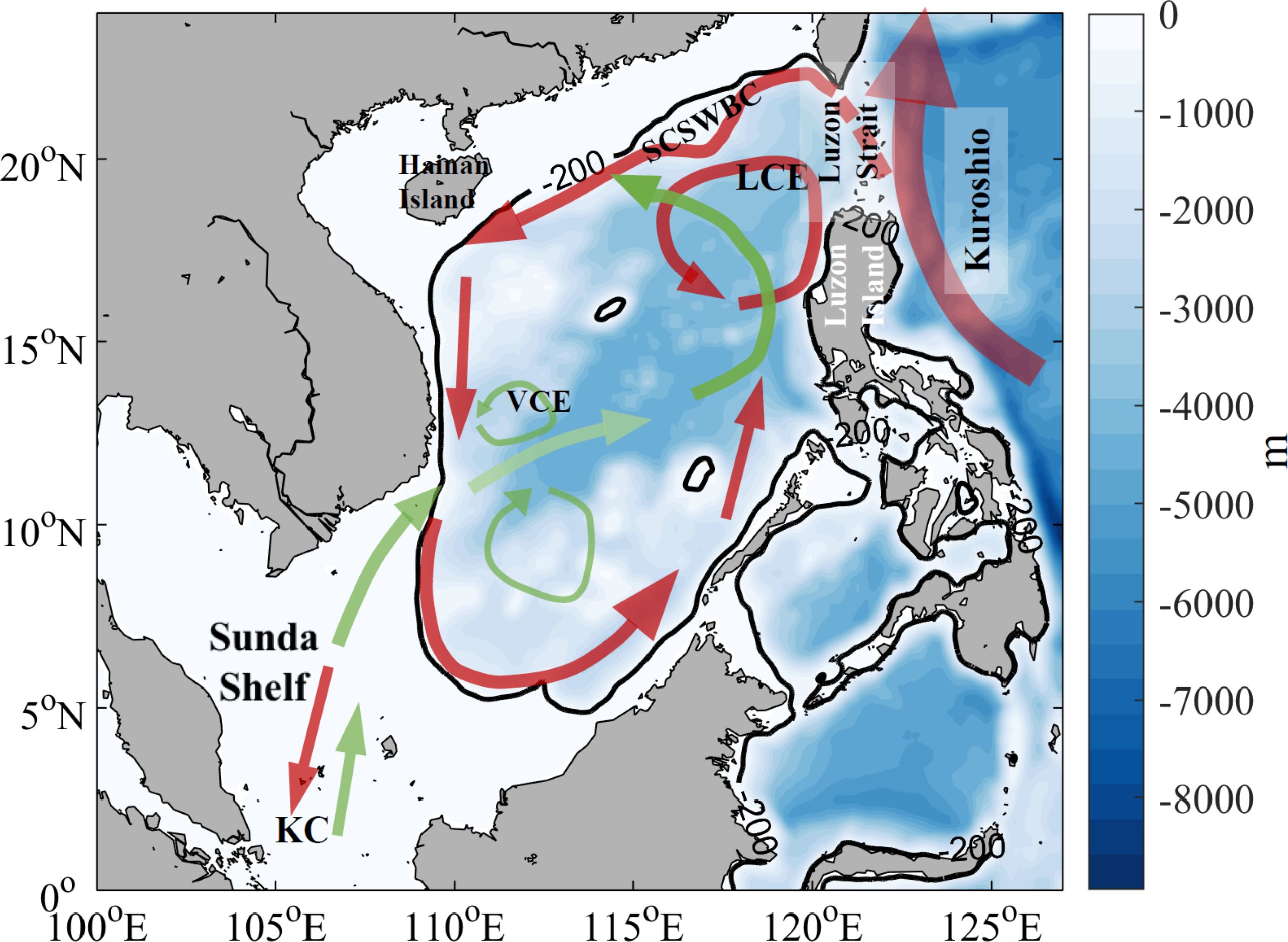
Figure 1. Diagram of the surface current patterns (based on data from Shu et al. 2018; Liu et al., 2008). Red (Green) means current pattern in winter (summer). LCE, Luzon Cold Eddy; SCSWBC, South China Sea Western Boundary Current; VCE, Vietnam Cold Eddy; KC, Karimata Current.

In the NSCS, Chl-a concentrations display a marked seasonal cycle, with high levels in winter and low levels in summer (Ning et al., 2004; Xian et al., 2012). The SCS connects to the Pacific Ocean through the Luzon Strait, allowing the Kuroshio to intrude into the SCS and contribute to its circulation (Xue et al., 2004; Qian et al., 2018; Cai et al., 2020). Winter phytoplankton blooms in Luzon Strait are often attributed to the interaction between monsoon-driven or current-induced upwelling, vertical mixing, meso-scale eddies, and fronts (Peñaflor et al., 2007; Shen et al., 2008; Wang et al., 2010, 2023; Shang et al., 2012; Lu et al., 2015; Xiu et al., 2016; Guo et al., 2017; Chang et al., 2022; Lao et al., 2023). The Luzon Cold Eddy, generally prevailed in winter and spring near the northwestern coast of Luzon Island, would alter the distribution of the Chl-a near the Luzon Island (Lu et al., 2015; Huang et al., 2019; Sun et al., 2023). During the summer, when the southwest monsoon prevails, upwelling and a northeastward jet are induced along the coast of Vietnam (Kuo, 2000; Fang et al., 2002; Xie et al., 2003; Lin et al., 2009; Ma et al., 2012). The upwelling elevates nutrients into shallow layers, supporting phytoplankton growth, resulting in the surface high Chl-a (Yang et al., 2012; Chen et al., 2021). With the transport of this jet in nutrients and biomass, the Chl-a off the east of the Vietnam significantly was enhanced. The interaction between cyclonic and anticyclonic eddies with the jet stream formed a high Chl-a belt (Liang et al., 2018).

There are several methods to measure Chl-a concentrations in the ocean, each with its own limitations. Traditionally, in situ ship-based, autonomous profiling float, and remote sensing satellites are the primary means of acquiring Chl-a data in the ocean (Kishino et al., 1997; Wright, 1997; Dierssen, 2010; Rykaczewski and Dunne, 2011; Boyce et al., 2012; Wernand et al., 2013). In situ ship-based and floats generally have low spatial or temporal resolution. Remote sensing satellite, offering high spatial and temporal resolution data, is easily affected by cloud cover (Shropshire et al., 2016). Considering the difficulties in acquiring the Chl-a, simulating the Chl-a or phytoplankton with marine ecological numerical model was an excellent method. However, the accuracy of numerical model results depends on the parameterization scheme of ecological (or biogeochemical) processes and the optimization of parameters. Developing a robust ocean ecological model requires substantial time for construction, calibration, and computation.

Recently, machine learning techniques, particularly deep learning, have advanced rapidly. The application of machine learning in ocean science has provided new insights into predicting key environmental or hydrodynamic indicators (Jouini et al., 2013; Aleshin et al., 2024; Krestenitis et al., 2024). Due to its strong capabilities in nonlinear regression, deep learning has been extensively utilized in oceanography, for tasks such as predicting sea surface temperature (SST), eddies, waves, and Chl-a (Liu et al., 2021; Liu and Li, 2023; Roussillon et al., 2023; Zhao et al., 2024). Ding and Li (2024) compared the performance of CNN, LSTM, and hybrid CNN-LSTM models for Chl-a prediction, concluding that the hybrid CNN-LSTM model outperformed standalone models with an R-squared, R² = 0.72. Similarly, Zhou et al. (2024) contributed further insights into the application of machine learning for ecological predictions. However, in some cases, machine-learning was not performed well than empirical algorithms. Bygate and Ahmed (2024) combined observational data and Landsat 8 surface reflectance to evaluate empirical and machine learning models for retrieving water quality indicators in Matagorda Bay, highlighting the limitations of traditional machine learning models in water quality inversion. Yang et al. (2024) developed a self-attention mechanism-based deep learning model to estimate nine phytoplankton pigment concentrations within the upper 300 m of the ocean, achieving R² > 0.8 and revealing a positive correlation between the maximum phytoplankton layer location and the Niño 3.4 index in the Equatorial Pacific Niño 3.4 region. Roussillon et al. (2023) introduced a multi-mode CNN to globally reconstruct phytoplankton biomass by learning region-specific responses to physical forcing. Their model achieved an R² > 0.87, highlighting the capacity of multi-mode approaches to uncover spatially consistent responses to ocean dynamic.

On the one hand, previous studies have revealed various complex dynamical processes related with the surface Chl-a in the SCS (Dai et al., 2022; Xian et al., 2012; Wang et al., 2023; Guo et al., 2017; Ma et al., 2012; Yu et al., 2019). On the other hand, machine learning has the advantage of finding complex nonlinear relationship among variables in an environmental setting (Song and Jiang, 2023). Hence, machine learning can provide a powerful support in elucidating the complex quantitative relationship between the physical factors (such as wind, SST) and the surface Chl-a. A few studies have used machine learning or deep learning to build a model link the physical factors and surface Chl-a with monthly data (Li et al., 2023; Roussillon et al., 2023). However, the possibility and performance by using the atmospheric and oceanic physical data to predict surface Chl-a with daily data remains unclear. This study discussed the feasibility of a predictive model based on the ResUnet architecture (Diakogiannis et al., 2020) to predict daily Chl-a concentrations in the SCS (100°E-124°E, 0°N-25°N) by atmospheric and oceanic dynamic factors. The ResUnet model enables the capture of the effects of multiple ocean dynamical processes on Chl-a evolution from the data. This approach yields accurate results while significantly reducing computational costs compared to traditional ocean ecological modeling methods.

2 Data and methods

2.1 Data

The dataset used in this study was derived from the atmosphere and ocean reanalysis datasets, European Centre for Medium-Range Weather Forecasts (ECMWF) Reanalysis v5 (ERA-5; https://www.ecmwf.int/en/forecasts/dataset/ecmwf-reanalysis-v5) and Hybrid Coordinate Ocean Model (HYCOM; https://www.hycom.org/). The 10 m wind fields were derived from the ERA-5, with spatial resolution as 0.25°×0.25° and the temporal resolution as 1-hourly. We calculated the mean value per 24 hours for acquiring the daily air forcing data to keep the same temporal resolution in our study. The SST, surface currents (eastward and northward velocity) and sea surface height (SSH) were derived from the HYCOM. The original spatial resolution is 0.08° and temporal resolution is 3-hourly. We interpolated the original data to the ERA-5 resolution and calculated the daily data every 8 times layer. These physical factors, such as wind, current, SSH, and SST, have been shown to be closely related to the variation in surface Chl-a in previous studies (Yu et al., 2019; Xiu et al., 2016; Geng et al., 2019).

This study focuses on discussing feasibility of a predictive model capable of forecasting future Chl-a concentrations by establishing a link between oceanic and atmospheric dynamic variables (e.g., wind fields, sea surface temperature, and current fields) and surface Chl-a. The predictive model requires complete and valid Chl-a as the label to ensure the effectiveness of the model. However, there is a number of missing values in the SCS from the remote sensing satellite data. Therefore, the Chl-a data used as the target variable (True) was derived from the Ye et al. (2024). The data covers the period from January 1, 2013, to December 31, 2017, with a temporal resolution of daily averages. This dataset was reconstructed using a combination of satellite and observational data, employing optimal interpolation and the SwinUnet method. Ye et al. (2024) successfully reconstructed a high-quality surface Chl-a dataset; however, the approach relies heavily on satellite remote sensing data, which limited the application in short-term prediction. In contrast, numerical models, such as HYCOM and ERA5, could provide oceanic and atmospheric dynamic factors, which can be leveraged to predict short-term variations in surface Chl-a. For this purpose, we considered the datasets from Ye et al. (2024) as the true Chl-a to train a model with physical factors. More information is listed in Table 1.

Table 1

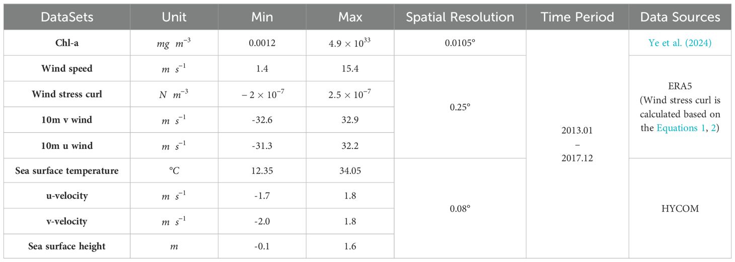
Table 1. Introduction of the datasets used in this study.

2.2 Methods

2.2.1 Data pre-processing

In order to achieve spatial resolution consistency across all predictor variables, we employed linear interpolation to adjust predictor variables from HYCOM to a resolution of 0.25° × 0.25°. Each predictor variable contained 97 × 101 data grid points, covering the period from 2013 to 2017. To maintain consistency among the variables, data standardization was applied. The daily predictor variables, represented as two-dimensional arrays of 97 × 101, were then concatenated to form a three-dimensional array with dimensions N × 97 × 101, with each variable occupying a separate channel within the data structure. In our experimental design, the predictors include data points for all available variables on a given day, which are subsequently used to forecast the Chl-a concentration (predictand) for that same day. To align the predictand data with the model output, Chl-a data was resampled to 0.25° × 0.25° before model training and was standardized thereafter. Following training, the model outputs were denormalized to retrieve the predicted Chl-a values. The experimental results demonstrated that this methodology effectively enhances the model’s fitting performance. The wind stress and wind stress curl in Table 1 are calculated as follows:

$\begin{array}{ll}\overrightarrow{\tau }=\rho C\overrightarrow{u}·\left|\overrightarrow{u}\right|& (1)\end{array}$

$\begin{array}{ll}\mathrm{\nabla }\times \overrightarrow{\tau }=\frac{\partial {\tau }_y}{\partial x}-\frac{\partial {\tau }_x}{\partial y}& (2)\end{array}$

The $\overrightarrow{u}$ is the wind vector, and $\overrightarrow{\tau }$ is the wind stress. ${\tau }_x$ and ${\tau }_y$ represent the eastward and northward component of the wind stress. The $\rho$ and C are the air density and drag coefficient, respectively. The C is estimated based on Large and Pond (1981).

2.2.2 Residual U-Net model

The UNet is a deep learning architecture for image segmentation that utilizes a symmetric encoder-decoder structure with skip connections to effectively capture and preserve detailed spatial information (Ronneberger et al., 2015). In this study, we employed a modified UNet architecture to enhance effectiveness, as shown in Figure 2. The model features a U-shaped structure with four encoder-decoder modules. To enhance the model’s ability to handle non-linear relationships, the traditional ReLU activation function was replaced with the Sigmoid Linear Unit (SiLU) activation function due to its advantage in smooth activation (Elfwing et al., 2017). To address overfitting and mitigate issues of exploding or vanishing gradients, Batch Normalization (BN) was applied after the convolutional layers. Furthermore, the AdamW optimizer was employed to improve training stability and performance by effectively managing weight decay (Loshchilov and Hutter, 2019). Consistent with most regression tasks, Mean Squared Error Loss (MSELoss) was utilized as the loss function. These modifications were implemented to collectively improve the model’s performance, accuracy, and computational efficiency.

Figure 2

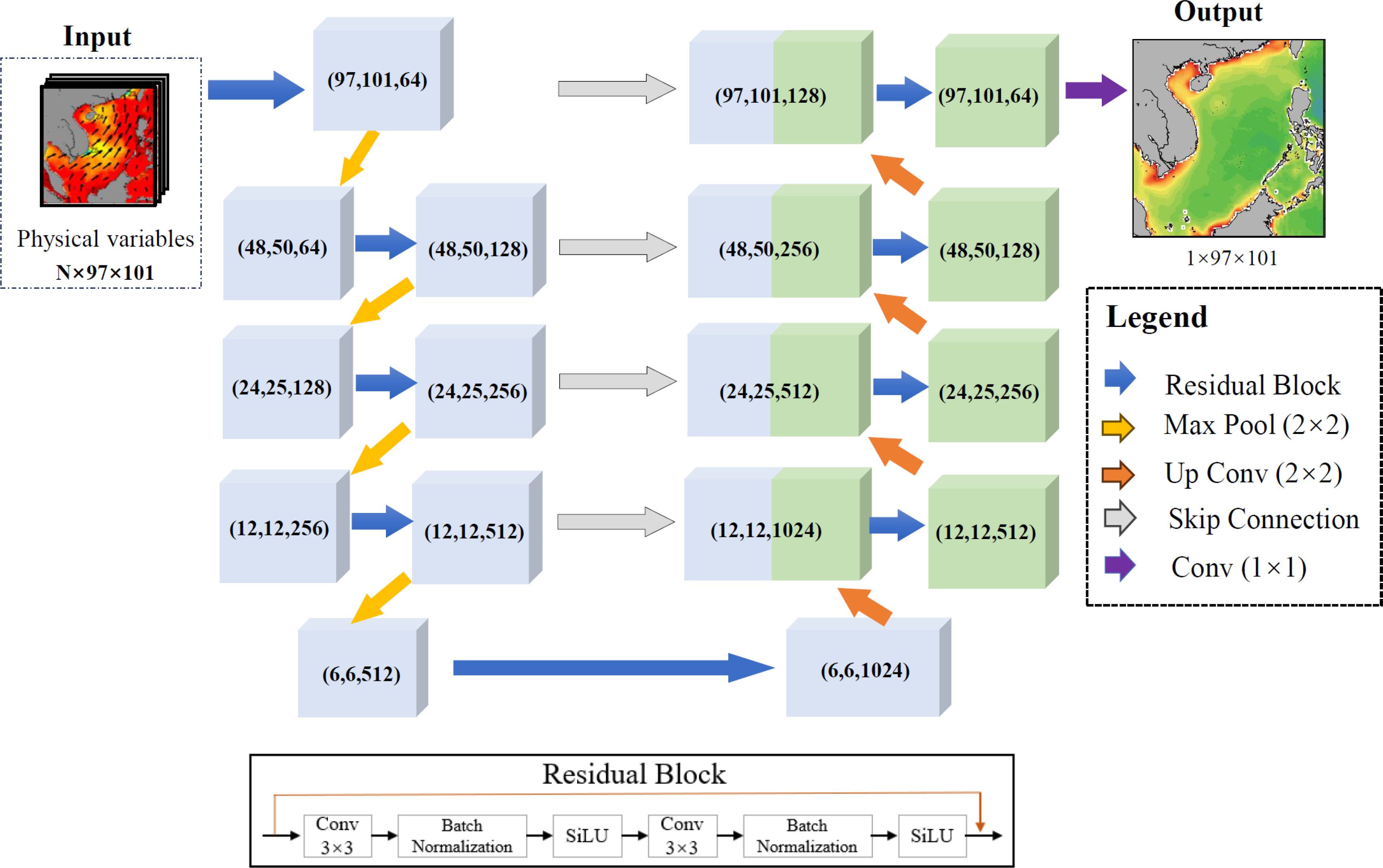
Figure 2. An illustration of the ResUNet architecture. Each colored cube symbolizes a feature map, with the numbers within the parentheses indicating the (width × height × channels).

The basic module of the UNet network is a residual module, each of which consists of two 3 × 3 two-dimensional convolutional layers, two BatchNorm2d layers, and two SiLU activation functions. The encoder part (left half of Figure 2) consists of a residual module and a max pooling layer. This configuration gradually reduces the feature mapping dimensions in length and width, thereby enhancing higher-order features. Following the encoder, the same number of decoders (right half of Figure 2) decode the features, including up-sampling to double the size of the feature map and skip connections. This process produces a feature map of size [64, 97, 101]. The final layer of the model is a 1 × 1 convolutional layer that reduces the number of channels to 1, producing the final 97 × 101 Chl-a outputs of the model. Definitions of deep learning terms, including Residual Block, SiLU, and max pooling, are provided in the Appendix.

2.2.3 Data split and model accuracy metrics

In this study, Chl-a data from 2013 to 2016 were allocated for model training, testing, and validation at proportions of 70%, 20%, and 10%, respectively. Data from 2017 was subsequently utilized to evaluate the model’s effectiveness in applications. There are some extremely large anomalies (> 10¹⁰) in Chl-a data from Ye et al. (2024). Therefore, during data preprocessing, we conducted thorough data cleaning and identified anomalies in the Chl-a data for a total of 26 days, which were removed to maintain the accuracy and consistency of the dataset. To comprehensively evaluate model performance, we employed three key metrics: the correlation coefficient (r), Root Mean Square Error (RMSE), and Mean Absolute Error (MAE). These metrics offer a quantitative assessment of the correlation and discrepancies between predicted and True data, thus providing valuable insights into the model’s performance and reliability.

1. Correlation Coefficient (r): It measures the strength and direction of the linear relationship between predicted and True values, calculated as:

$$r=\frac{\sum (y_i-\overline{y})({\widehat{y}}_i-\overline{\widehat{y}})}{\sqrt{\sum {(y_i-\overline{y})}^2}\sqrt{\sum {({\widehat{y}}_i-\overline{\widehat{y}})}^2}}$$

2. Root Mean Square Error (RMSE): RMSE quantifies the average deviation of predictions from actual values, given by:

$$\text{RMSE}=\sqrt{\frac{1}{n}{\displaystyle \sum _{i=1}^n}{(y_i-{\widehat{y}}_i)}^2}$$

3. Mean Absolute Error (MAE): MAE provides a straightforward interpretation of the average prediction error:

$$\text{MAE}=\frac{1}{n}\sum _{i=1}^n|y_i-{\widehat{y}}_i|$$

The symbols used in the equations are defined as follows: $y_i$ represents the True value, ${\widehat{y}}_i$ denotes the predicted value, $\overline{y}$ is the mean of the True values, $\overline{\widehat{y}}$ is the mean of the predicted values, and n refers to the number of observations. It is already known that there is a certain correlation between atmospheric and oceanic dynamic data and surface Chl-a in the SCS (Yu et al., 2019). The temporal and spatial variation of Chl-a are influenced by factors such as wind fields, ocean currents, and SST. To test the accuracy of model in different predictors, we conducted two sets of experiments: (1) using 10 m wind field, wind speed, wind stress curl, and SST (Exp1), and (2) using 10 m wind field, wind speed, wind stress curl, SST, surface current, and SSH (Exp2). In the SCS, wind fields and SST are strongly correlated with surface Chl-a (Yu et al., 2019). Therefore, the goal of the Exp1 was to explore the feasibility of building a robust model. On the other hand, surface current and SSH are related to the horizontal advection process and vertical structure of density to some extent (e.g., mesoscale eddies), which, to some extent, influence the distribution of nutrients and phytoplankton (Xiu et al., 2016). The goal of the Exp2 was to explore the performance of the model when considering the currents and SSH.

3 Results and discussion

3.1 Model evaluation using statistical indicators

The comparisons between predicted and true Chl-a concentrations of two experiments based on the Chl-a from 2013 to 2016, separated into three parts (training, testing, and validation sets), are shown in Figure 3. In general, the data points are primarily distributed along the 1:1 line, with correlation coefficients between predicted and true Chl-a exceeding 0.9 across all datasets (Figure 3). It indicated that both Exp1 and Exp2 could well predict the surface Chl-a in the SCS. However, there were some discrepancies in performances between these two experiments. The Exp2 showing higher correlation coefficient (Figures 3a–f) among training (0.929 in Exp1 versus 0.935 in Exp2), testing (0.911 in Exp1 vs 0.918 in Exp2) and validation datasets (0.913 in Exp1 versus 0.925 in Exp2). And the RMSE of Exp2 were 0.1, 0.112, and 0.107 for the training, testing, and validation datasets, respectively (Figures 3d–f). It also indicated that the deviation between the predicted values and the true values of the model is smaller. The comparison of MAE between Exp1 and Exp2 also denoted the Exp2 might be better. Li et al. (2023) employed four machine learning methods to predict the Chl-a using physical factors with Random Forests demonstrating the best performance (R² ~ 0.8). Aleshin et al. (2024) applied LightGBM and ResNet-18 to predict the Chl-a with an R² ~ 0.7. Roussillon et al. (2023) used a multi-mode convolutional neural network to reconstruct satellite-derived Chl-a with monthly physical drivers, such as SST, with R² ~ 0.85. In comparison, our model exhibited superior performance in predicting the Chl-a in the SCS.

Figure 3

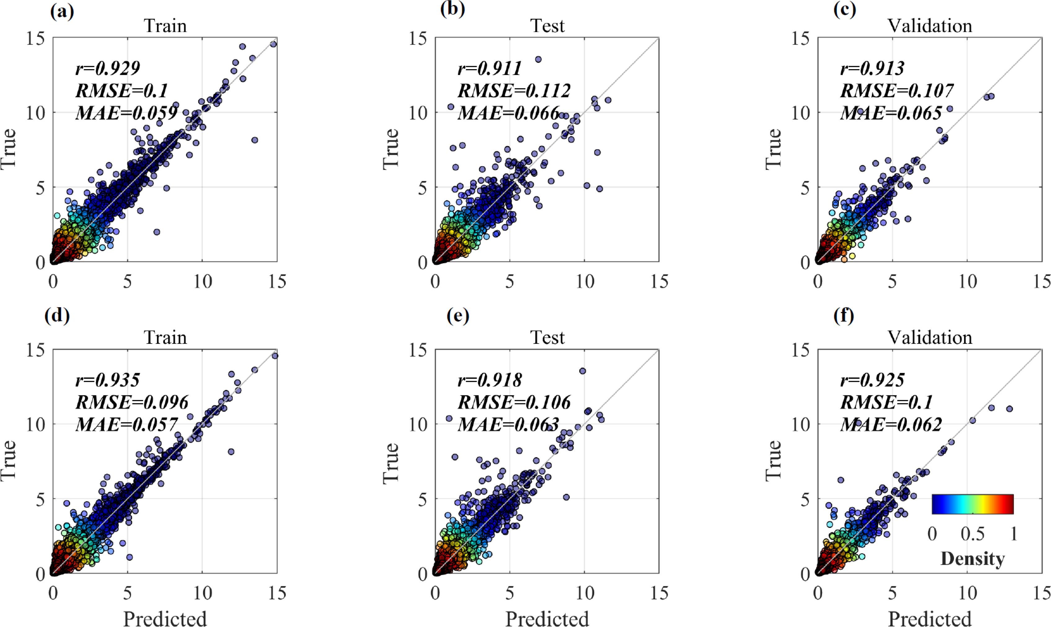
Figure 3. Scatter plots between predicted and the counterpart locations of the True Chl-a in training (a, d), testing (b, e), and validation (c, f). The first (second) row represents Exp1 (Exp2).

Further, the residuals between predicted and true Chl-a, separated into training, testing, and validation sets, from 2013 to 2016 were calculated and shown in Figure 4. The results showed that frequency of the residuals shown normal distribution (Figure 4). The average of the residuals is -0.00039, -0.00095, -0.00045 for training, testing, and validation datasets in Exp1, respectively (Figures 4a–c). While the averages of the residuals are -0.00015, -0.00163, and -0.00061 for training, testing, and validation datasets in Exp2, respectively (Figures 4d–f). Although the mean residuals in Exp2 was less than Exp1, both Exp1 and Exp2 had small mean residuals (< 1%), which indicated a good performance of the model without significant systematic bias. This reflected the robustness and reliability of the model in capturing the surface Chl-a. In addition, the $\sigma$ were about 0.14, 0.22, and 0.21 for training, testing, and validation datasets in Exp1, respectively (Figures 4a–c). They were slightly higher than the corresponding parts in Exp2 (Figures 4d–f). It denotes the results of Exp2 are more stable compared to the result of Exp1.

Figure 4

Figure 4. Frequency plots with x-axis as residuals (model results – True value) in training (a, d), testing (b, e), and validation (c, f). The first (second) row represents Exp1 (Exp2).

3.2 Model evaluation in terms of Chl-a temporal and spatial distributions

The model performance was evaluated using correlation coefficients, RMSE, and MAE, all of which indicated good performance for this deep learning model. Experimental results suggested that surface currents (eastward and northward velocities) and SSH slightly enhance the model’s performance. The model’s ability to predict the spatial distribution and seasonal variation of surface Chl-a requires further evaluation.

To represent seasonal variations (Spring, Summer, Autumn, and Winter), surface Chl-a values from the validation dataset on the dates 2013/03/05, 2013/06/15, 2013/09/28, and 2013/12/11 were selected. Figure 5 illustrates the spatial distributions of Chl-a for these selected dates across the true, Exp1, and Exp2. Generally, surface Chl-a exhibits high concentrations on the shelf, particularly along the coast, and low concentrations in the basin of the SCS (Liu et al., 2002, 2012; Shen et al., 2008; Fang et al., 2014). The high Chl-a on the shelf is typically attributed to riverine inputs, such as nutrients, biomass, terrestrial transport, and upwelling (Li et al., 2018; Lu and Gan, 2015). Both the Exp1 and Exp2 effectively captured the prominent feature of the higher Chl-a along the coast and lower Chl-a in the basin (Figures 5e–l).

Figure 5

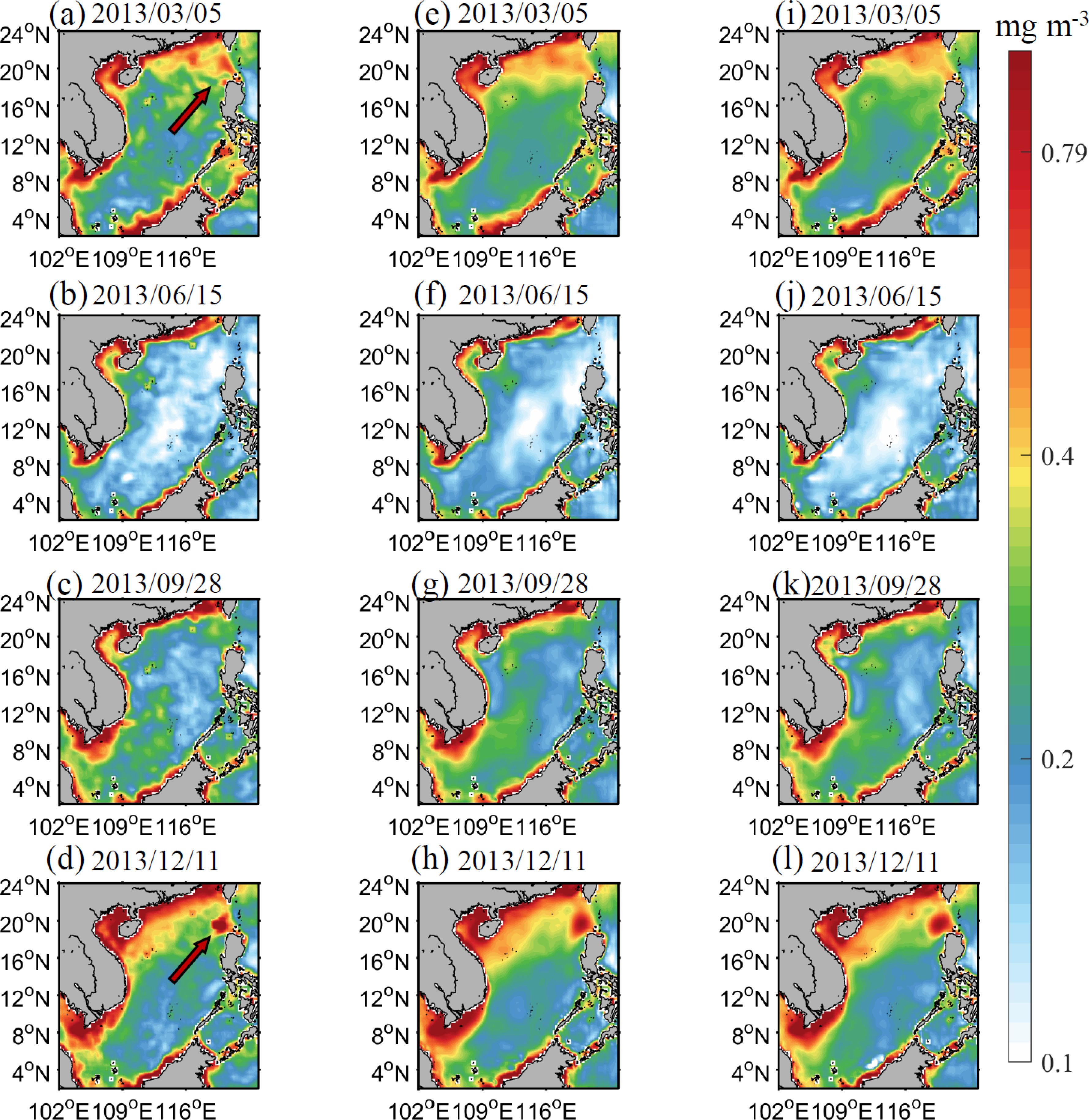
Figure 5. Spatial distributions of Chl-a in 2013/03/05 (a, e, i), 2013/06/15 (b, f, j); 2013/09/28 (c, g, k); 2013/12/11 (d, h, l). The first column is the true Chl-a, while the second and third column represent Chl-a in Exp1 and Exp2, respectively.

Meanwhile, seasonal Chl-a variation were exhibited significantly (Figures 5a–d). Along the coast, the area with high Chl-a (e.g., > 0.4) were more prominent in the Spring and Winter (Figures 5a, d), while they were lower in the Summer and Autumn (Figures 5b, c). And the Chl-a in the basin were lowest during the Summer (Figures 5b). This feature was also captured by the model in both Exp1 and Exp2 (Figures 5f, j). Additionally, the Luzon Strait, as a major pathway between the Pacific and the SCS, shows significant blooms in winter and spring when northeasterly winds prevail (Peñaflor et al., 2007; Shen et al., 2008). The true Chl-a data includes a notable phytoplankton bloom on the western side of the Luzon Strait (see arrow in Figures 5a, d). Both Exp1 and Exp2 predicted similar phytoplankton blooms, although the area might be slightly larger.

In terms of the overall Chl-a distribution, both Exp1 and Exp2 successfully captured the high Chl-a on the shelf and low Chl-a in the basin, and the seasonal variation of the surface Chl-a. They also reproduced the relatively high Chl-a concentration on the northwest side of Luzon Island (Figures 5e, h, i, l) in Spring and Winter. Based on the evaluation of the Chl-a spatial pattern and seasonal variation, the two experiments demonstrated good performance.

3.3 Spatial distribution of temporal correlation coefficients

The model well captured the spatial pattern and seasonal variation of the Chl-a in both Exp1 and Exp2. However, the temporal correlation between true Chl-a and model predicted Chl-a was unclear. To evaluate the model’s performance in capturing Chl-a temporal variation, the Pearson correlation coefficients between true Chl-a and model predicted Chl-a for each grid were calculated (Figure 6). Figure 6 illustrates the spatial distribution of correlation coefficients in training (Figures 6a, d), testing (Figures 6b, e), and validation (Figures 6c, f).

Figure 6

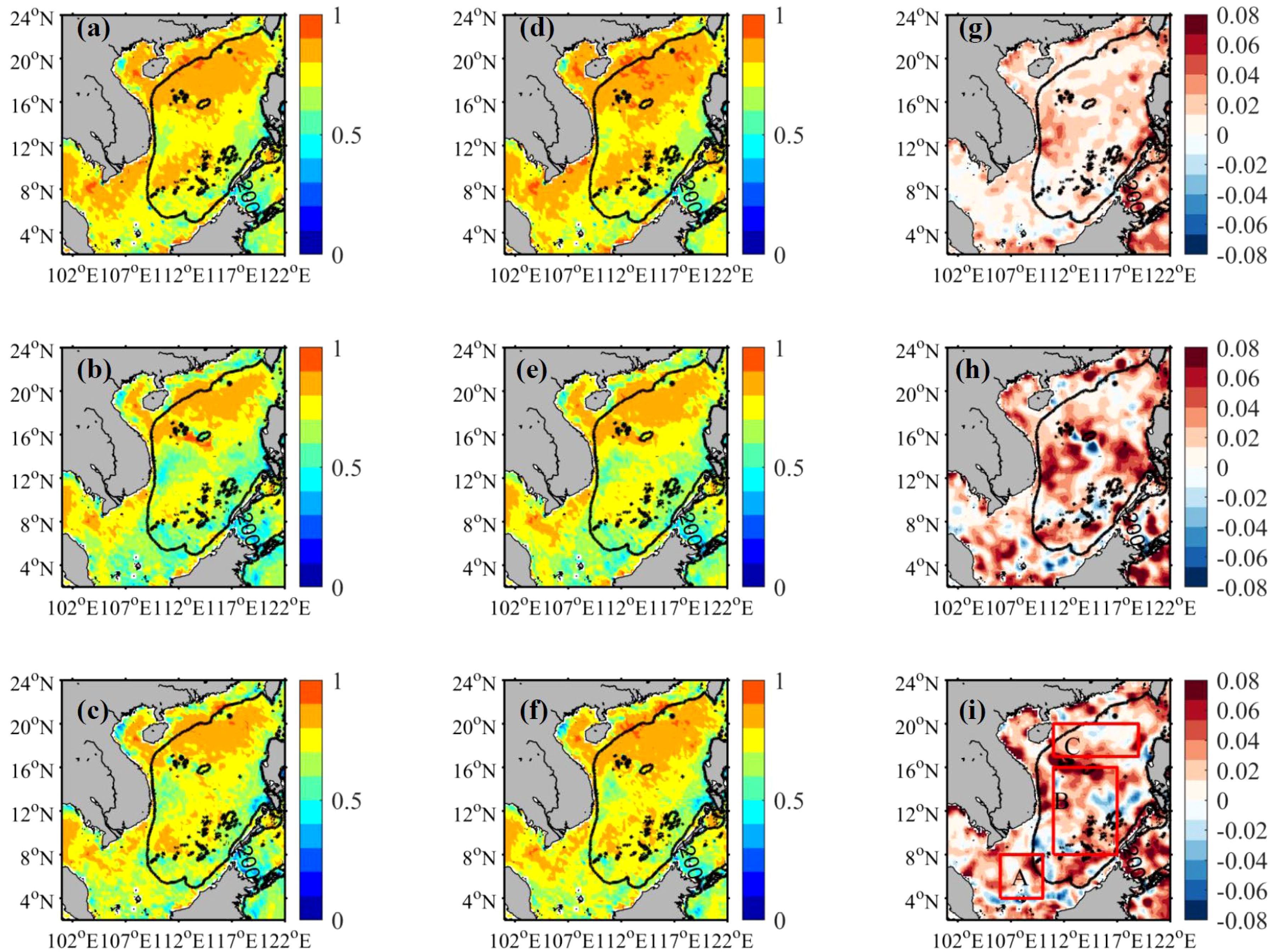
Figure 6. Spatial distributions of Pearson correlation coefficients (with p < 0.05) in training (a, d), testing (b, e), and validation (c, f) datasets. The (g–i) were, $\Delta r$, calculated by (d) minus (a), (e) minus (b), and (f) minus (c), respectively. The first column represents Exp1 (Exp2). Boxes A, B, and C in (i) covered the NSCS, central SCS, and Sunda Shelf.

In general, the correlation coefficients in the training dataset (Figures 6a, d) were the highest, which is reasonable given that the training dataset was used to train the model. Regarding the spatial pattern of the correlation coefficients, whether in the Exp1 or Exp2, the values to the north of 16°N were notably higher than those to the south of 16°N in training, testing, and validation (Figures 6a–f). Specifically, the correlation coefficients in the NSCS were generally above 0.8, while in the SSCS, they typically ranged from 0.6 ~ 0.8, with the highest values observed in the training dataset (Figures 6a, d). This discrepancy might be caused by the strength of the relationship between physical factors and surface Chl-a in the NSCS and SSCS. Significant seasonal and inter-seasonal variability of Chl-a is observed in the NSCS (Shen et al., 2008; Palacz et al., 2011; Tang et al., 2014), which is generally associated with the seasonal dynamics of factors such as the monsoon and Kuroshio intrusion (Xue et al., 2004; Xian et al., 2012; Chang et al., 2022; Sun et al., 2023). Previous studies have shown a high correlation between SST and Chl-a (Shen et al., 2008; Tang et al., 2014; Yu et al., 2019). In summer, the mixed layer depth (MLD) is shallow, and the presence of strong stratification due to high SST and weaker winds inhibits the supply of nutrient-rich subsurface water. However, in winter, the MLD usually deepens due to intensified northeasterly monsoons and buoyancy flux, accompanied by a reduction in SST (Tang et al., 2003). As the MLD deepens, nutrient-rich water from the subsurface is transported to the surface layer. With sufficient nutrient support, phytoplankton flourishes during winter. Consequently, Exp1 performs well in capturing the temporal variability of surface Chl-a in NSCS (Figures 6a–c). However, in the SSCS, Geng et al. (2019) revealed that wind- and buoyancy-induced mixing are less intense in the central SCS than in the NSCS, limiting vertical nutrient transport to above the subsurface Chl-a maximum layer. This may explain the lower correlation coefficients in the SSCS (Figures 6a–f).

In respect of the comparison between Exp1 and Exp2, the correlation coefficients in the Exp2 were generally slightly higher than that in the Exp1 in the SCS (Figures 6g–i). However, in the Exp1, the correlation coefficients in the NSCS were comparable with those of Exp2, especially in the training dataset, with increasing correlation coefficients less than 0.03 (Figures 6g–i). It indicated that atmospheric data and SST are crucial factors for simulating the Chl-a in the NSCS. However, between 12°N and 16°N, Exp2 performed well in capturing the temporal variation of Chl-a, with $\text{Δ}r$ ($r_{Exp2}-r_{Exp1}$) exceeding 0.04 (Figures 6h, i). Generally, Exp2 performed better than Exp1, although there were small areas with decreased correlation coefficients to the south of 16°N. In the basin of SSCS, the correlation coefficients were higher than that on the shelf. For Exp1, the correlation coefficient in the Sunda Shelf were not as strong as in Exp2, with r < 0.7 (Figure 6c). However, the Exp2 showed slightly improvement in the Sunda Shelf with slightly higher r (Figure 6i). Comparisons between Exp1 and Exp2 demonstrated that the model achieved the best performance when SSH and currents were included as an input variable, especially in the SSCS.

3.4 Model performance in capturing local important features

We evaluated the model based on spatial distribution of Chl-a and the temporal correlation by Pearson correlation coefficients between true Chl-a and model predicted Chl-a. It denoted the performance of the model was excellent, especially for the NSCS. However, the model’s ability to reproduce local spatial characteristics of Chl-a required further assessment. We selected typical high surface Chl-a patches near the Luzon Strait, Hainan Island, and Vietnam (see red arrows in Figures 7a, d, g) to validate the model’s ability in capturing details from validation datasets (2014/01/30, 2013/10/20, 2014/7/23). Figures 7a, d showed a high surface Chl-a patch surrounded by low surface Chl-a. Previous studies have demonstrated that cold eddies contribute to this phenomenon (Wang et al., 2010; Lu et al., 2015; Sun et al., 2023). In fact, these high Chl-a patches were generally closed to the cold eddies, as indicated by SSH (0.4 contours in Figures 7a, d). Off the coast of Vietnam, high Chl-a concentrations usually followed the jet during the summer (Liang et al., 2018), as shown in Figure 7g (see red arrow). The high Chl-a patch off the Vietnam closely matched the location of the strengthened current velocity.

Figure 7

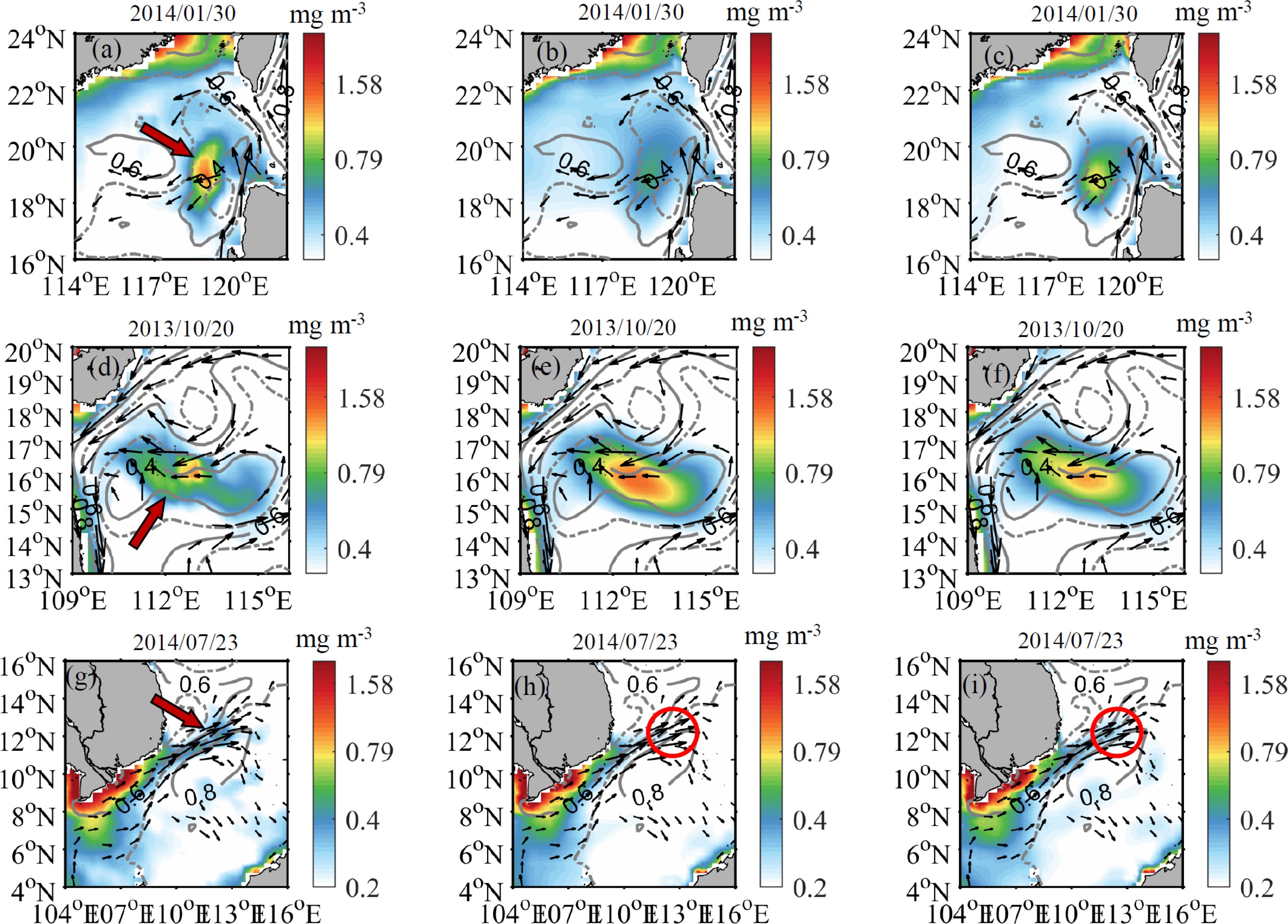
Figure 7. Spatial distributions of Chl-a snapshots in the True (a, d, g) and Validation datasets (b, c, e, f, h, i). The second and third columns show surface Chl-a in Exp1 and Exp2, respectively. The gray contours represent SSH (0.1 m interval between solid and dashed contours), and the black arrows indicate velocity, exceeding 0.4 m s⁻¹, vectors in HYCOM.

Both Exp1 and Exp2 captured the main features of these high Chl-a patches. To the northwest of Luzon Island, while Exp1 predicted high Chl-a patch (Figure 7b), the Chl-a concentration was not as high as in Figure 7a. However, Exp2 performed better in simulating this patch with higher Chl-a concentration closed to the 0.4 contour (Figure 7c), although it was still lower than that in Exp1. In addition, to the northwest of the high Chl-a patch, the Chl-a concentration was higher than in the True Chl-a (Figures 7a, b). Nonetheless, Exp2 provided a better prediction of Chl-a distribution (Figure 7c) in this area as True Chl-a (Figure 7a). Similarly, the high Chl-a patches near 112°E, 16°N, predicted by the Exp1 and Exp2, were different (Figures 7e, f). The Chl-a concentration in Exp1 was higher than in the True Chl-a (Figure 7d) and Exp2 (Figure 7f). The high Chl-a derived from Exp2 was more comparable to that in the true Chl-a (Figures 7d, f). East of Vietnam, high surface Chl-a is generally induced by upwelling and a southwesterly wind-driven jet (Qiu et al., 2011; Liu et al., 2012; Gao et al., 2013; Chen et al., 2014, 2021). A snapshot of high Chl-a extending from the coast to the east of Vietnam, aligned with the jet (indicated by the strengthened velocity), was shown in Figure 7g. Our model successfully reproduced the high Chl-a along the jet (Figures 7h, i), although the concentrations were not as pronounced as those in the true Chl-a (see red arrow in Figure 7g). Exp2 demonstrated a better prediction of Chl-a along the jet, with higher Chl-a concentrations (see red circles in Figure 7h, i).

This comparison between Exp1 and Exp2 demonstrated that additional variables, SSH and currents, are beneficial to predict the details of the Chl-a distribution. To some extent, the spatial distribution of SSH reflects vertical information, such as the thermocline. Approximately 28.7 cyclonic eddies and 27.9 anticyclonic eddies occur annually in the SCS, which significantly influence the ecosystem of the SCS (Xiu et al., 2010). Mesoscale eddies played a significant role in modulating surface Chl-a through eddy advection, eddy pumping, eddy trapping, and eddy-induced Ekman pumping in the SCS (Gaube et al., 2014; Xiu et al., 2016). Eddy pumping played an important role in controlling surface Chl-a variability to the west of the Luzon Strait and northwest of Luzon Island (Xiu et al., 2016). Yu et al. (2019) found that sea level anomalies are highly correlated with surface Chl-a. Meanwhile, Xiu et al. (2016) revealed that horizontal eddy advection highly influenced the Chl-a off the Vietnam coast. Therefore, including SSH and advection as model inputs enabled the predicted data to more effectively reproduce surface Chl-a.

3.5 Application of the model in 2017

The model trained in Exp2 was further applied to predict surface Chl-a in 2017. Based on model performance in the NSCS and SSCS (Figure 6), spatially averaged Chl-a in Boxes A, B, and C was used to assess temporal variability. The predicted Chl-a largely captured the magnitude and temporal variability of surface Chl-a across Boxes A, B, and C (Figures 8a-1, b-1, c-1). Model performance, as measured by correlation coefficients, was highest in the NSCS, followed by the Sunda Shelf and the central SCS (Figures 8a-2, b-2, c-2). Although the model effectively reproduced the temporal variability of surface Chl-a, particularly the seasonal cycle, its performance was relatively less accurate for daily-scale Chl-a variations, as indicated by the distribution of observed Chl-a (Figures 8a-1, b-1, c-1). To improve model validation, we further calculated 8-day averaged surface Chl-a and compared predicted values with observed Chl-a. On the 8-day scale, correlation coefficients between predicted and observed Chl-a were higher than those on the daily scale (Figures 8d-2, e-2, f-2). Observed Chl-a data aligned more closely with predicted values, and both RMSE and MAE indicated reduced errors in 8-day averaged results (Figures 8d-1, e-1, f-1).

Figure 8

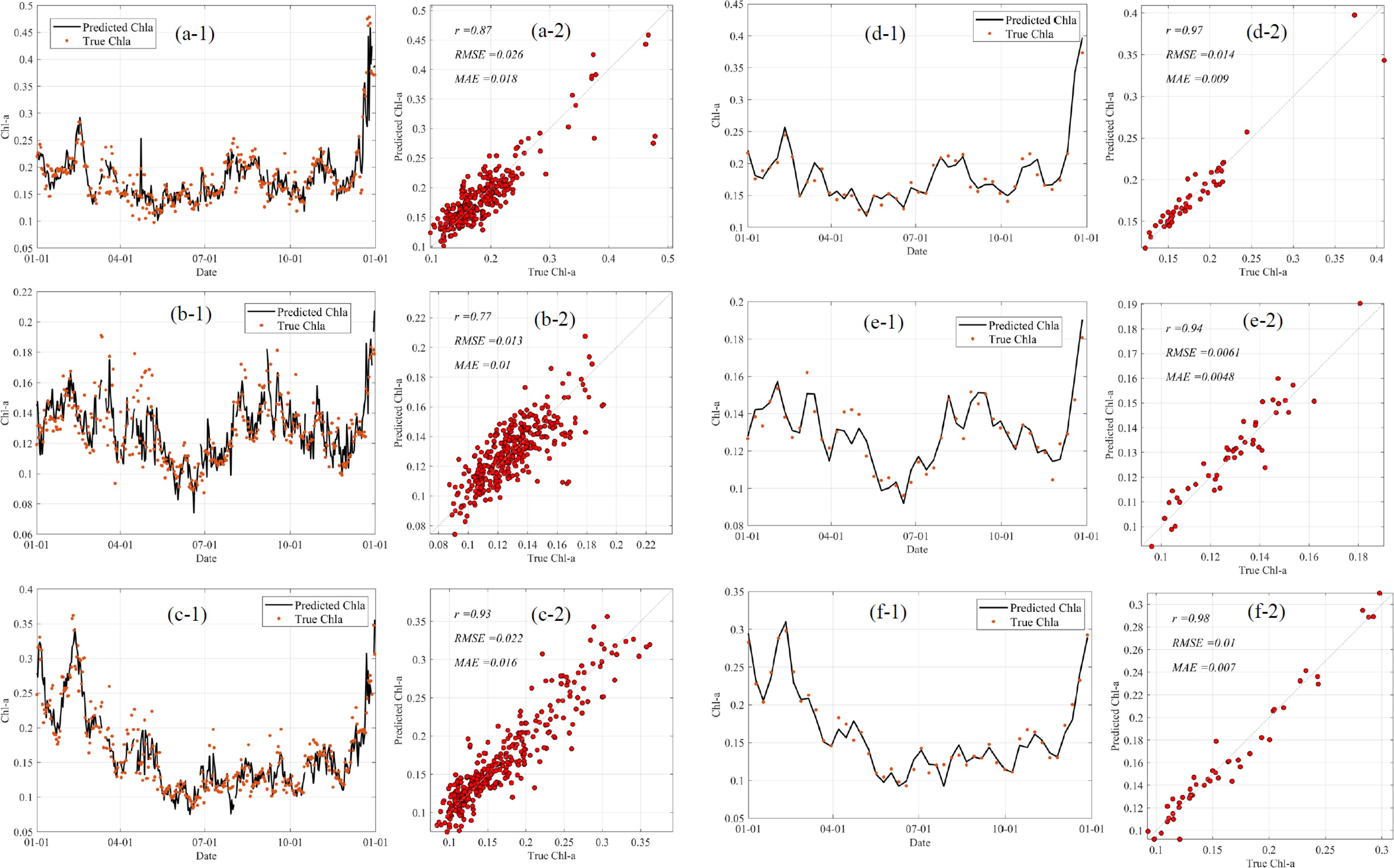
Figure 8. Time series of daily spatially averaged Chl-a (units: mg m^-3) in Box A (a-1), B (b-1), and C (c-1), along with their corresponding scatter plots of true versus predicted Chl-a in Box A (a-2), B (b-2), and C (c-2). Panels (d-1), (e-1), and (f-1) represent the 8-day averaged Chl-a and their corresponding scatter plots of true versus predicted Chl-a [(d-2), (e-2), and (f-2)] in Boxes A, B, and C, respectively. The location of boxes is in Figure 6i.

One possible reason for the reduced daily-scale accuracy was that daily variations in surface Chl-a were more complex than those on longer timescales. Small-scale dynamic processes, such as fronts and submesoscale eddies, played an essential role in vertical nutrient transport (Callbeck et al., 2017; Jing et al., 2021; Zheng and Jing, 2022). However, the horizontal resolution of model inputs may limit the model’s ability to capture these small-scale features, affecting day-scale performance. Additionally, surface Chl-a is often associated with vertical nutrients distribution (Geng et al., 2019; Liu et al., 2020), but obtaining continuous, widespread data on nutrient distribution in the vertical direction remains challenging. These factors constrain the model’s precision in predicting daily-scale Chl-a variability.

4 Conclusion

In this study, we developed a statistical model based on the ResUnet architecture to predict daily Chl-a in the SCS through atmospheric and oceanic physical data. The strong correlation between the model-predicted and true Chl-a demonstrates that the model performed well in estimating surface Chl-a. It supported the feasibility of predicting surface Chl-a based on atmospheric and oceanic data.

The model performed better in the NSCS than in the SSCS. In the NSCS, the combination of atmospheric factors and SST was sufficient to reproduce the temporal variability in Chl-a. This superior performance can likely be attributed to the strong correlation between SST and surface Chl-a in this region. In the SSCS, the model-predicted variability of Chl-a had better performance in Exp2, which denoted that the oceanic dynamic factors, such as surface currents and SSH, played a vital role in estimating the Chl-a in the SSCS using deep learning methods.

While the model moderately captured the spatial distribution features in Chl-a when considering only wind-related variables and SST, its performance improved significantly when oceanic dynamic data were included. The addition of surface currents and SSH enabled the model to accurately represent areas with elevated Chl-a due to eddies, particularly around the Luzon Strait and the southeastern side of Hainan Island. The SSH is generally associated with eddies, which enhances the ability of model to predict elevated Chl-a resulting from eddies. In conclusion, the incorporation of ocean dynamics into ecological prediction models based on deep learning technology offers effectively ways and enhances the accuracy of Chl-a predictions in the SCS.

Data availability statement

Publicly available datasets were analyzed in this study. This data can be found here: ERA-5: https://www.ecmwf.int/en/forecasts/dataset/ecmwf-reanalysis-v5; HYCOM: https://www.hycom.org/; Chla: https://doi.org/10.5281/zenodo.10478524.

Author contributions

WF: Conceptualization, Data curation, Formal analysis, Investigation, Methodology, Writing – original draft, Writing – review & editing. AL: Conceptualization, Data curation, Formal analysis, Investigation, Methodology, Writing – original draft, Writing – review & editing. HJ: Supervision, Writing – review & editing. CS: Conceptualization, Supervision, Validation, Writing – review & editing. PX: Supervision, Funding acquisition, Writing – review & editing.

Funding

The author(s) declare financial support was received for the research, authorship, and/or publication of this article. This work is financially supported by the National Key Research and Development Program of China (2023YFF0805004, 2022YFE0136600 and 2022YFC3105303), the National Natural Science Foundation of China (42376154), Huanggang Normal University (No. 2042023053), Guangdong Basic and Applied Basic Research Foundation (2022A1515240069 and 2024A1515012032). The work was supported by the Outstanding Postdoctoral Scholarship, State Key Laboratory of Marine Environmental Science at Xiamen University. The work would not have been possible without the free and open access to Chlorophyll-a data, and we sincerely thank the Shilin Tang Team at the South China Sea Institute of Oceanography, Chinese Academy of Sciences, for their invaluable assistance with this work. Also, we gratefully thank the HYCOM consortium for providing the HYCOM data, and the European Centre for Medium-Range Weather Forecasts (ECMWF) for the ERA data, which were invaluable to this research. Special thanks are due to the reviewers of the manuscript.

Conflict of interest

The authors declare that the research was conducted in the absence of any commercial or financial relationships that could be construed as a potential conflict of interest.

Generative AI statement

The author(s) declare that no Generative AI was used in the creation of this manuscript.

Publisher’s note

All claims expressed in this article are solely those of the authors and do not necessarily represent those of their affiliated organizations, or those of the publisher, the editors and the reviewers. Any product that may be evaluated in this article, or claim that may be made by its manufacturer, is not guaranteed or endorsed by the publisher.

References

Aleshin M., Illarionova S., Shadrin D., Ivanov V., Vanovskiy V., Burnaev E. (2024). Machine learning-based modeling of chl-a concentration in Northern marine regions using oceanic and atmospheric data. Front. Mar. Sci. 11. doi: 10.3389/fmars.2024.1412883

Crossref Full Text | Google Scholar

Boyce D. G., Lewis M., Worm B. (2012). Integrating global chlorophyll data from 1890 to 2010. Limnol. Oceanogr. Methods 10, 840–852. doi: 10.4319/lom.2012.10.840

Crossref Full Text | Google Scholar

Bygate M., Ahmed M. (2024). Monitoring water quality indicators over Matagorda Bay, Texas, using Landsat-8. Remote Sens. 16, 1120. doi: 10.3390/rs16071120

Crossref Full Text | Google Scholar

Cai Z., Gan J., Liu Z., Hui C. R., Li J. (2020). Progress on the formation dynamics of the layered circulation in the South China Sea. Prog. Oceanogr. 181, 102246. doi: 10.1016/j.pocean.2019.102246

Crossref Full Text | Google Scholar

Callbeck C. M., Lavik G., Stramma L., Kuypers M. M. M., Bristow L. A. (2017). Enhanced nitrogen loss by Eddy-induced vertical transport in the offshore Peruvian oxygen minimum zone. PloS One 12, e0170059. doi: 10.1371/journal.pone.0170059

PubMed Abstract | Crossref Full Text | Google Scholar

Chang Y., Shih Y.-Y., Tsai Y.-C., Lu Y.-H., Liu J. T., Hsu T.-Y., et al. (2022). Decreasing trend of kuroshio intrusion and its effect on the chlorophyll-a concentration in the Luzon Strait, South China Sea. GISci. Remote Sens. 59, 633–647. doi: 10.1080/15481603.2022.2051384

Crossref Full Text | Google Scholar

Chen Y. L. (2005). Spatial and seasonal variations of nitrate-based new production and primary production in the South China Sea. Deep Sea Res. Part I 52, 319–340. doi: 10.1016/j.dsr.2004.11.001

Crossref Full Text | Google Scholar

Chen Y., Shi H., Zhao H. (2021). Summer phytoplankton blooms induced by upwelling in the Western South China Sea. Front. Mar. Sci. 8. doi: 10.3389/fmars.2021.740130

Crossref Full Text | Google Scholar

Chen G., Xiu P., Chai F. (2014). Physical and biological controls on the summer chlorophyll bloom to the east of Vietnam. J. Oceanogr. 70, 323–328. doi: 10.1007/s10872-014-0232-x

Crossref Full Text | Google Scholar

Chu P. C., Edmons N. L., Fan C. (1999). Dynamical mechanisms for the South China Sea seasonal circulation and thermohaline variabilities. J. Phys. Oceanogr. 29, 2971–2989. doi: 10.1175/1520-0485(1999)029<2971:DMFTSC>2.0.CO;2

Crossref Full Text | Google Scholar

Dai M., Su J., Zhao Y., Hofmann E. E., Cao Z., Cai W.-J., et al. (2022). Carbon fluxes in the coastal ocean: synthesis, boundary processes, and future trends. Annu. Rev. Earth Planet. Sci. 50, 593–626. doi: 10.1146/annurev-earth-032320-090746

Crossref Full Text | Google Scholar

Diakogiannis F. I., Waldner F., Caccetta P., Wu C. (2020). ResUNet-a: A deep learning framework for semantic segmentation of remotely sensed data. ISPRS J. Photogramm. Remote Sens. 162, 94–114. doi: 10.1016/j.isprsjprs.2020.01.013

Crossref Full Text | Google Scholar

Dierssen H. M. (2010). Perspectives on empirical approaches for ocean color remote sensing of chlorophyll in a changing climate. Proc. Natl. Acad. Sci. U.S.A. 107, 17073–17078. doi: 10.1073/pnas.0913800107

PubMed Abstract | Crossref Full Text | Google Scholar

Ding W., Li C. (2024). Algal blooms forecasting with hybrid deep learning models from satellite data in the Zhoushan fishery. Ecol. Inf. 82, 102664. doi: 10.1016/j.ecoinf.2024.102664

Crossref Full Text | Google Scholar

Elfwing S., Uchibe E., Doya K. (2017).Sigmoid-weighted linear units for neural network function approximation in reinforcement learning. Available online at: http://arxiv.org/abs/1702.03118 (Accessed November 3, 2024).

PubMed Abstract | Google Scholar

Fang W., Fang G., Shi P., Huang Q., Xie Q. (2002). Seasonal structures of upper layer circulation in the southern South China Sea from in situ observations. J. Geophys. Res. 107, 21–23. doi: 10.1029/2002JC001343

Crossref Full Text | Google Scholar

Fang M., Ju W., Liu X., Yu Z., Qiu F. (2014). Surface chlorophyll-a concentration spatio-temporal variations in the northern South China Sea detected using MODIS data. Terr. Atmos. Ocean. Sci. 26, 319–329. doi: 10.3319/TAO.2014.11.14.01(Oc

Crossref Full Text | Google Scholar

Fang G., Wang G., Fang Y., Fang W. (2012). A review on the South China Sea western boundary current. Acta Oceanol. Sin. 31, 1–10. doi: 10.1007/s13131-012-0231-y

Crossref Full Text | Google Scholar

Fang G., Wang Y., Wei Z., Fang Y., Qiao F., Hu X. (2009). Interocean circulation and heat and freshwater budgets of the South China Sea based on a numerical model. Dynam. Atmos. Oceans 47, 55–72. doi: 10.1016/j.dynatmoce.2008.09.003

Crossref Full Text | Google Scholar

Fernández-González C., Tarran G. A., Schuback N., Woodward E. M. S., Arístegui J., Marañón E. (2022). Phytoplankton responses to changing temperature and nutrient availability are consistent across the tropical and subtropical Atlantic. Commun. Biol. 5, 1035. doi: 10.1038/s42003-022-03971-z

PubMed Abstract | Crossref Full Text | Google Scholar

Gan J., Li H., Curchitser E. N., Haidvogel D. B. (2006). Modeling South China Sea circulation: Response to seasonal forcing regimes. J. Geophys. Res. 111, C06034. doi: 10.1029/2005JC003298

Crossref Full Text | Google Scholar

Gao S., Wang H., Liu G., Li H. (2013). Spatio-temporal variability of chlorophyll a and its responses to sea surface temperature, winds and height anomaly in the western South China Sea. Acta Oceanol. Sin. 2, 48–58. doi: 10.1007/s13131-013-0266-8

Crossref Full Text | Google Scholar

Gaube P., McGillicuddy D. J., Chelton D. B., Behrenfeld M. J., Strutton P. G. (2014). Regional variations in the influence of mesoscale eddies on near-surface chlorophyll. J. Geophys. Res. Oceans 119, 8195–8220. doi: 10.1002/2014JC010111

Crossref Full Text | Google Scholar

Geng B., Xiu P., Shu C., Zhang W., Chai F., Li S., et al. (2019). Evaluating the roles of wind- and buoyancy flux-induced mixing on phytoplankton dynamics in the northern and central South China Sea. J. Geophys. Res. Oceans 124, 680–702. doi: 10.1029/2018JC014170

Crossref Full Text | Google Scholar

Guo L., Xiu P., Chai F., Xue H., Wang D., Sun J. (2017). Enhanced chlorophyll concentrations induced by kuroshio intrusion fronts in the northern South China Sea. Geophys. Res. Lett. 44, 11,565–11,572. doi: 10.1002/2017GL075336

Crossref Full Text | Google Scholar

Huang Z., Zhuang W., Hu J., Huang B. (2019). Observations of the Luzon cold Eddy in the northeastern South China Sea in May 2017. J. Oceanogr. 75, 415–422. doi: 10.1007/s10872-019-00510-z

Crossref Full Text | Google Scholar

Jing Z., Fox-Kemper B., Cao H., Zheng R., Du Y. (2021). Submesoscale fronts and their dynamical processes associated with symmetric instability in the northwest Pacific subtropical ocean. J. Phys. Oceanogr. 51, 83–100. doi: 10.1175/JPO-D-20-0076.1

Crossref Full Text | Google Scholar

Jouini M., Lévy M., Crépon M., Thiria S. (2013). Reconstruction of satellite chlorophyll images under heavy cloud coverage using a neural classification method. Remote Sens. Environ. 131, 232–246. doi: 10.1016/j.rse.2012.11.025

Crossref Full Text | Google Scholar

Kishino M., Ishizaka J., Saitoh S., Senga Y., Utashima M. (1997). Verification plan of ocean color and temperature scanner atmospheric correction and phytoplankton pigment by moored optical buoy system. J. Geophys. Res. 102, 17197–17207. doi: 10.1029/96JD04008

Crossref Full Text | Google Scholar

Krestenitis M., Androulidakis Y., Krestenitis Y. (2024). Deep learning-based forecasting of sea surface temperature in the interim future: application over the Aegean, Ionian, and Cretan Seas (NE Mediterranean Sea). Ocean Dyn. 74, 149–168. doi: 10.1007/s10236-023-01595-3

Crossref Full Text | Google Scholar

Kuo N. (2000). Satellite observation of upwelling along the western coast of the South China Sea. Remote Sens. Environ. 74, 463–470. doi: 10.1016/S0034-4257(00)00138-3

Crossref Full Text | Google Scholar

Lao Q., Liu S., Wang C., Chen F. (2023). Global warming weakens the ocean front and phytoplankton blooms in the Luzon Strait over the past 40 years. J. Geophys. Res. Biogeo. 128, e2023JG007726. doi: 10.1029/2023JG007726

Crossref Full Text | Google Scholar

Large W. G., Pond S. (1981). Open ocean momentum flux measurements in moderate to strong winds. J. Phys. Oceanogr. 11, 324–336. doi: 10.1175/1520-0485(1981)011<0324:OOMFMI>2.0.CO;2

Crossref Full Text | Google Scholar

Li A., Shao T., Zhang Z., Fang W., Li W., Xu J., et al. (2023). Improvement in spatiotemporal Chl-a data in the South China Sea using the random-forest-based geo-imputation method and ocean dynamics data. J. Mar. Sci. Eng. 12, 13. doi: 10.3390/jmse12010013

Crossref Full Text | Google Scholar

Li Q. P., Zhou W., Chen Y., Wu Z. (2018). Phytoplankton response to a plume front in the northern South China Sea. Biogeosciences 15, 2551–2563. doi: 10.5194/bg-15-2551-2018

Crossref Full Text | Google Scholar

Liang W., Tang D., Luo X. (2018). Phytoplankton size structure in the western South China Sea under the influence of a ‘jet-eddy system. J. Marine. Syst. 187, 82–95. doi: 10.1016/j.jmarsys.2018.07.001

Crossref Full Text | Google Scholar

Lin I.-I., Wong G. T. F., Lien C., Chien C., Huang C., Chen J. (2009). Aerosol impact on the South China Sea biogeochemistry: An early assessment from remote sensing. Geophys. Res. Lett. 36, 2009GL037484. doi: 10.1029/2009GL037484

Crossref Full Text | Google Scholar

Liu K.-K., Chao S.-Y., Shaw P.-T., Gong G.-C., Chen C.-C., Tang T. Y. (2002). Monsoon-forced chlorophyll distribution and primary production in the South China Sea: observations and a numerical study. Deep-Sea Res. I 49, 1387–1412. doi: 10.1016/S0967-0637(02)00035-3

Crossref Full Text | Google Scholar

Liu Q., Kaneko A., Jilan S. (2008). Recent progress in studies of the South China Sea circulation. J. Oceanogr. 64, 753–762. doi: 10.1007/s10872-008-0063-8

Crossref Full Text | Google Scholar

Liu Y., Li X. (2023). Impact of surface and subsurface-intensified eddies on sea surface temperature and chlorophyll a in the northern Indian Ocean utilizing deep learning. Ocean Sci. 19, 1579–1593. doi: 10.5194/os-19-1579-2023

Crossref Full Text | Google Scholar

Liu X., Wang J., Cheng X., Du Y. (2012). Abnormal upwelling and chlorophyll-a concentration off South Vietnam in summer 2007. J. Geophys. Res. 117, 2012JC008052. doi: 10.1029/2012JC008052

Crossref Full Text | Google Scholar

Liu J., Wang Y., Yuan Y., Xu D. (2020). The response of surface chlorophyll to mesoscale eddies generated in the eastern South China Sea. J. Oceanogr. 76, 211–226. doi: 10.1007/s10872-020-00540-y

Crossref Full Text | Google Scholar

Liu F., Zhang T., Ye H., Tang S. (2021). Using satellite remote sensing to study the effect of sand excavation on the suspended sediment in the Hong Kong-Zhuhai-Macau Bridge region. Water 13, 435. doi: 10.3390/w13040435

Crossref Full Text | Google Scholar

Loshchilov I., Hutter F. (2019).Decoupled weight decay regularization. Available online at: http://arxiv.org/abs/1711.05101 (Accessed November 3, 2024).

Google Scholar

Lu W., Yan X., Jiang Y. (2015). Winter bloom and associated upwelling northwest of the Luzon Island: A coupled physical-biological modeling approach. J. Geophys. Res.: Oceans 120, 533–546. doi: 10.1002/2014JC010218

Crossref Full Text | Google Scholar

Lu Z., Gan J. (2015). Controls of seasonal variability of phytoplankton blooms in the Pearl River Estuary. Deep Sea Research Part II: Topical Studies in Oceanography. 117, 86–96. doi: 10.1016/j.dsr2.2013.12.011

Crossref Full Text | Google Scholar

Ma J., Liu H., Zhan H., Lin P., Du Y. (2012). Effects of chlorophyll on upper ocean temperature and circulation in the upwelling regions of the South China Sea. Aquat. Ecosyst. Health Manage. 15, 127–134. doi: 10.1080/14634988.2012.687663

Crossref Full Text | Google Scholar

Ning X., Chai F., Xue H., Cai Y., Liu C., Shi J. (2004). Physical-biological oceanographic coupling influencing phytoplankton and primary production in the South China Sea. J. Geophys. Res. 109, 2004JC002365. doi: 10.1029/2004JC002365

Crossref Full Text | Google Scholar

Palacz A. P., Xue H., Armbrecht C., Zhang C., Chai F. (2011). Seasonal and inter-annual changes in the surface chlorophyll of the South China Sea. J. Geophys. Res. 116, C09015. doi: 10.1029/2011JC007064

Crossref Full Text | Google Scholar

Peñaflor E. L., Villanoy C. L., Liu C.-T., David L. T. (2007). Detection of monsoonal phytoplankton blooms in Luzon Strait with MODIS data. Remote Sens. Environ. 109, 443–450. doi: 10.1016/j.rse.2007.01.019

Crossref Full Text | Google Scholar

Qian S., Wei H., Xiao J., Nie H. (2018). Impacts of the Kuroshio intrusion on the two eddies in the northern South China Sea in late spring 2016. Ocean Dynam. 68, 1695–1709. doi: 10.1007/s10236-018-1224-y

Crossref Full Text | Google Scholar

Qiu F., Fang W., Fang G. (2011). Seasonal-to-interannual variability of chlorophyll in central western South China Sea extracted from SeaWiFS. Chin. J. Ocean. Limnol. 29, 18–25. doi: 10.1007/s00343-011-9931-y

Crossref Full Text | Google Scholar

Qu T. (2000). Upper-layer circulation in the South China Sea. J. Phys. Oceanogr. 30, 1450–1460. doi: 10.1175/1520-0485(2000)030<1450:ULCITS>2.0.CO;2

Crossref Full Text | Google Scholar

Ronneberger O., Fischer P., Brox T. (2015). “U-Net: Convolutional Networks for Biomedical Image Segmentation,” in Medical Image Computing and Computer-Assisted Intervention – MICCAI 2015. Eds. Navab N., Hornegger J., Wells W. M., Frangi A. F. (Cham: Springer International Publishing), 234–241. doi: 10.1007/978-3-319-24574-4_28

Crossref Full Text | Google Scholar

Roussillon J., Fablet R., Gorgues T., Drumetz L., Littaye J., Martinez E. (2023). A Multi-Mode Convolutional Neural Network to reconstruct satellite-derived chlorophyll-a time series in the global ocean from physical drivers. Front. Mar. Sci. 10. doi: 10.3389/fmars.2023.1077623

Crossref Full Text | Google Scholar

Rykaczewski R. R., Dunne J. P. (2011). A measured look at ocean chlorophyll trends. Nature 472, E5–E6. doi: 10.1038/nature09952

PubMed Abstract | Crossref Full Text | Google Scholar

Shang S., Li L., Li J., Li Y., Lin G., Sun J. (2012). Phytoplankton bloom during the northeast monsoon in the Luzon Strait bordering the Kuroshio. Remote Sens. Environ. 124, 38–48. doi: 10.1016/j.rse.2012.04.022

Crossref Full Text | Google Scholar

Shen S., Leptoukh G. G., Acker J. G., Zuojun Y., Kempler S. J. (2008). Seasonal variations of chlorophyll a concentration in the northern South China Sea. IEEE Geosci. Remote Sens. Lett. 5, 315–319. doi: 10.1109/LGRS.2008.915932

Crossref Full Text | Google Scholar

Shropshire T., Li Y., He R. (2016). Storm impact on sea surface temperature and chlorophyll a in the Gulf of Mexico and Sargasso Sea based on daily cloud-free satellite data reconstructions. Geophys. Res. Lett. 43, 12199–12207. doi: 10.1002/2016GL071178

Crossref Full Text | Google Scholar

Shu Y., Wang Q., Zu T. (2018). Progress on shelf and slope circulation in the northern South China Sea. Sci. China Earth Sci. 61, 560–571. doi: 10.1007/s11430-017-9152-y

Crossref Full Text | Google Scholar

Song Y., Jiang H. (2023). A deep learning–based approach for empirical modeling of single-point wave spectra in open oceans. J. Phys. Oceanogr. 53, 2089–2103. doi: 10.1175/JPO-D-22-0198.1

Crossref Full Text | Google Scholar

Sun R., Li P., Gu Y., Zhou C., Liu C., Zhang L. (2023). Seasonal variation of the shape and location of the Luzon cold eddy. Acta Oceanol. Sin. 42, 14–24. doi: 10.1007/s13131-022-2084-3

Crossref Full Text | Google Scholar

Tang D., Kawamura H., Lee M.-A., Van Dien T. (2003). Seasonal and spatial distribution of chlorophyll-a concentrations and water conditions in the Gulf of Tonkin, South China Sea. Remote Sens. Environ. 85, 475–483. doi: 10.1016/S0034-4257(03)00049-X

Crossref Full Text | Google Scholar

Tang S., Liu F., Chen C. (2014). Seasonal and intraseasonal variability of surface chlorophyll a concentration in the South China Sea. Aquat. Ecosyst. Health Manage. 17, 242–251. doi: 10.1080/14634988.2014.942590

Crossref Full Text | Google Scholar

Wang X., Du Y., Zhang Y., Wang T. (2023). Effects of multiple dynamic processes on chlorophyll variation in the Luzon Strait in summer 2019 based on glider observation. J. Ocean. Limnol. 41, 469–481. doi: 10.1007/s00343-022-1416-7

Crossref Full Text | Google Scholar

Wang J., Tang D., Sui Y. (2010). Winter phytoplankton bloom induced by subsurface upwelling and mixed layer entrainment southwest of Luzon Strait. J. Marine. Syst. 83, 141–149. doi: 10.1016/j.jmarsys.2010.05.006

Crossref Full Text | Google Scholar

Wernand M. R., van der Woerd H. J., Gieskes W. W. C. (2013). Trends in ocean colour and chlorophyll concentration from 1889 to 2000, worldwide. PloS One 8, e63766. doi: 10.1371/journal.pone.0063766

PubMed Abstract | Crossref Full Text | Google Scholar

Wright P. N. (1997). “Real-time chlorophyll and nutrient data from a new marine data buoy in Southampton Water, UK,” in Seventh International Conference on Electronic Engineering in Oceanography - Technology Transfer from Research to Industry (IEE, Southampton, UK), 73–78. doi: 10.1049/cp:19970665

Crossref Full Text | Google Scholar

Xian T., Sun L., Yang Y.-J., Fu Y.-F. (2012). Monsoon and eddy forcing of chlorophyll-a variation in the northeast South China Sea. Int. J. Remote Sens. 33, 7431–7443. doi: 10.1080/01431161.2012.685970

Crossref Full Text | Google Scholar

Xie S., Xie Q., Wang D., Liu W. T. (2003). Summer upwelling in the South China Sea and its role in regional climate variations. J. Geophys. Res. 108, 2003JC001867. doi: 10.1029/2003JC001867

Crossref Full Text | Google Scholar

Xiu P., Chai F., Shi L., Xue H., Chao Y. (2010). A census of eddy activities in the South China Sea during 1993–2007. J. Geophys. Res. 115, 2009JC005657. doi: 10.1029/2009JC005657

Crossref Full Text | Google Scholar

Xiu P., Guo M., Zeng L., Liu N., Chai F. (2016). Seasonal and spatial variability of surface chlorophyll inside mesoscale eddies in the South China Sea. Aquat. Ecosyst. Health Manage. 19, 250–259. doi: 10.1080/14634988.2016.1217118

Crossref Full Text | Google Scholar

Xue H., Chai F., Pettigrew N., Xu D., Shi M., Xu J. (2004). Kuroshio intrusion and the circulation in the South China Sea. J. Geophys. Res. 109, 2002JC001724. doi: 10.1029/2002JC001724

Crossref Full Text | Google Scholar

Yang Y., Li X., Li X. (2024). A self-attention-based deep learning model for estimating global phytoplankton pigment profiles. IEEE Trans. Geosci. Remote Sens. 62, 1–15. doi: 10.1109/TGRS.2024.3435044

Crossref Full Text | Google Scholar

Yang Y. J., Xian T., Sun L., Fu Y. F. (2012). Summer monsoon impacts on chlorophyll-a concentration in the middle of the South China Sea: climatological mean and annual variability. Atmos. Oceanic Sci. Lett. 5, 15–19. doi: 10.1080/16742834.2012.11446961

Crossref Full Text | Google Scholar

Ye H., Yang C., Dong Y., Tang S., Chen C. (2024). A daily reconstructed chlorophyll- a dataset in the South China Sea from MODIS using OI-SwinUnet. Earth Syst. Sci. Data 16, 3125–3147. doi: 10.5194/essd-16-3125-2024

Crossref Full Text | Google Scholar

Yu Y., Xing X., Liu H., Yuan Y., Wang Y., Chai F. (2019). The variability of chlorophyll-a and its relationship with dynamic factors in the basin of the South China Sea. J. Marine. Syst. 200, 103230. doi: 10.1016/j.jmarsys.2019.103230

Crossref Full Text | Google Scholar

Zhao Q., Peng S., Wang J., Li S., Hou Z., Zhong G. (2024). Applications of deep learning in physical oceanography: a comprehensive review. Front. Mar. Sci. 11. doi: 10.3389/fmars.2024.1396322

Crossref Full Text | Google Scholar

Zheng R., Jing Z. (2022). Submesoscale-enhanced filaments and frontogenetic mechanism within mesoscale eddies of the South China Sea. Acta Oceanol. Sin. 41, 42–53. doi: 10.1007/s13131-021-1971-3

Crossref Full Text | Google Scholar

Zhou G., Chen J., Liu M., Ma L. (2024). A spatiotemporal attention-augmented ConvLSTM model for ocean remote sensing reflectance prediction. Int. J. Appl. Earth Observ. Geoinform. 129, 103815. doi: 10.1016/j.jag.2024.103815

Crossref Full Text | Google Scholar

Appendix A. terms in deep learning method used in this study

● Feature: In the context of deep learning, a feature represents an individual measurable attribute or characteristic that can be used to describe and analyze an observation or phenomenon.

● Batch Normalization (BatchNorm) Layer: This layer standardizes the inputs of each minibatch, which enhances the stability and efficiency of the training process by reducing internal covariate shift.

● Convolutional Layer: The convolutional layer applies a set of filters to the input data, producing feature maps that capture spatial hierarchies and patterns. This layer performs the convolution operation by sliding the filters over the input and computing the dot product between the filter and the input data, which is fundamental for feature extraction in convolutional neural networks.

● Max Pooling Layer: This layer decreases the spatial dimensions of the input feature maps by extracting the maximum value from each sub-region. Max pooling aids in minimizing computational complexity and mitigating overfitting.

● Sigmoid Linear Unit (SiLU) Activation Function: The SiLU activation function, also known as the Swish function, is defined as:

$$\text{SiLU}(x)=x·\sigma (x)$$

where $\sigma (x)$ is the sigmoid function, given by:

$$\sigma (x)=\frac{1}{1+e^{-x}}$$

It combines the properties of linear and sigmoid functions, allowing for smooth, non-linear transformations that can improve the training dynamics of neural networks. The SiLU function has been shown to perform well in various deep learning tasks due to its ability to enhance gradient flow and adaptively control the output.

● Residual Connection: A residual connection bypasses one or more intermediate layers, directly feeding the output of one layer to subsequent layers. This technique aids in training deeper networks by alleviating the vanishing gradient problem.

● Skip Connection: A skip connection, also known as a shortcut connection, involves bypassing one or more layers in the neural network and directly passing the output from an earlier layer to a deeper layer.

● Up-Sampling: In the UNet architecture, up-sampling is employed in the expansive path to restore the resolution of the feature maps. This step is essential for reconstructing high-resolution outputs from lower-resolution feature representations.

● Down-Sampling: Down-sampling decreases the spatial dimensions of the input feature maps, commonly used in the contracting path of the UNet. This process simplifies the information, enabling the model to capture more global features in the earlier layers.

● AdamW Optimizer: The AdamW optimizer is an extension of the Adam optimization algorithm that incorporates weight decay directly into the optimization process. Unlike traditional Adam, which applies weight decay as part of the regularization term added to the loss, AdamW decouples weight decay from the optimization steps, leading to better regularization and improved training dynamics.