Characterizing wind, wave, and Stokes drift interactions in the upper ocean during Typhoon Doksuri using the COAWST model

The COAWST model is used in this study to simulate wind fields, wave fields, and Stokes drift during Typhoon Doksuri, aiming to reveal the dynamics of atmosphere-ocean-wave interactions under typhoon conditions. The COAWST model provides a more accurate simulation of typhoon wind speeds compared to ERA5 reanalysis data and the WRF model, and it offers a more precise representation of significant wave heights (Hs) than ERA5 reanalysis data and the SWAN model. The root mean square error (RMSE) of wind speed shows a reduction of 90.97% and 61.09% compared to ERA5 and WRF, respectively, resulting in an RMSE of 1.71 m/s. While the Hs correlation coefficient is 0.86. Comparative analysis indicates that COAWST has higher accuracy than WRF and ERA5, particularly in capturing the asymmetrical phenomena of wind and wave field. The high-value regions of the wind and wave fields are concentrated in the first quadrant around the typhoon center. The COAWST model output, combined with empirical orthogonal function (EOF) analysis and the Ekman-Stokes number, is used to quantitatively evaluate the contributions of wind and wave effects to ocean surface flow. The peak Stokes drift velocity reaches 0.73 m/s, with a maximum transport intensity of 13 m²/s and a transport depth of 20 meters. EOF analysis indicates that the first two modes explain over 88% of the Stokes transport. The first mode represents the spatial distribution of Stokes drift during the typhoon, while the second mode captures the temporal evolution of drift velocity. This study provides insight into atmosphere-ocean interactions during extreme weather conditions by using the COAWST model to analyze Stokes drift and its influence on ocean surface dynamics.

1 Introduction

In recent years, significant progress has been made in typhoon research, focusing on typhoon intensity, track prediction, and environmental influences on typhoon development. Refining initial conditions and enhancing model resolution were shown to improve the accuracy of intensity predictions for Typhoon Haiyan (Chen et al., 2014). Simulations of Typhoon Megi revealed that initial storm intensity and size significantly influenced cyclone tracks, with stronger initial conditions leading to an earlier northward turn (Wang et al., 2017). Typhoons rank among the most destructive global meteorological phenomena, causing profound impacts on ocean surface flow due to intense wind stress (Inagaki et al., 2020; Lin and Wu, 2021). A comparative study on Typhoons Lekima and Muifa examined the relationship between typhoon intensity, wave height, and storm surge, revealing a linear increase in maximum Hs and storm surge with typhoon intensity (Wang et al., 2022). The WRF model is widely used for typhoon simulations, providing crucial insights into wind dynamics and storm intensity. When coupled with the SWAN model, WRF effectively simulates typhoon waves and their coastal interactions (Luo et al., 2023). However, the performance of the WRF model is sensitive to the choice of physical parameterizations, which vary depending on the typhoon’s track and environmental conditions (Davis et al., 2008; Lee et al., 2016). These findings collectively advance the understanding of typhoon intensity, track, and environmental interactions and provide a theoretical basis for refining numerical model configurations and improving prediction accuracy.

Significant progress has been made in understanding the effects of waves under typhoon conditions, especially their impact on upper ocean mixing, storm surge, and air-sea interactions. Wave breaking during Typhoons Haiyan and Jebi was found to enhance typhoon intensity (Zhao et al., 2017). Simulations of Typhoon Kalmaegi using a coupled model emphasized the critical role of atmosphere-ocean feedback in reconstructing the typhoon-affected environment (Lim Kam Sian et al., 2020). Extreme wave heights in the Northwest Pacific were shown to be significantly influenced by typhoons during summer and autumn, with an asymmetric wind field distribution leading to enhanced wave height on the right side of the typhoon track and weaker waves on the left (Woo and Park, 2021; Wu et al., 2023; Zheng et al., 2023). The importance of model grid resolution and wave interactions in simulating extreme waves was also highlighted, with findings showing that wave interactions are crucial for improving simulation accuracy (Hsiao et al., 2023). Overall, these studies provide valuable insights into the impact of waves on the marine environment under typhoon conditions, particularly in terms of upper ocean mixing, heat flux exchange, and storm surge dynamics, contributing significant scientific value.

Stokes drift, a key manifestation of wave nonlinear effects, is particularly significant under typhoon conditions (van den Bremer and Breivik, 2018). Waves were shown to enhance boundary layer mixing due to their impact on turbulence in the Ekman layer (McWilliams et al., 2012). Langmuir turbulence studies under hurricane conditions found that Stokes drift played a crucial role in enhancing turbulence (Rabe et al., 2015). In the western Mediterranean, Stokes drift contributed up to 15% to wind-driven transport under wind-wave conditions (Sayol et al., 2016). Long-term observational data revealed that Stokes drift aligned with wind stress direction, primarily driven by local wind waves (Clarke and Van Gorder, 2018). Climate system model studies demonstrated that Stokes drift and non-breaking waves improved simulations of sea surface temperature and mixed layer depth (Cunningham et al., 2022; Fan et al., 2023). Under typhoon conditions, Stokes drift significantly enhanced vertical mixing, impacting mixed layer depth and vertical temperature distribution (Yu et al., 2024). Overall, these studies indicate that Stokes drift significantly influences upper ocean mixing, wind stress distribution, and material transport under wind-wave conditions, especially during typhoons and intense storms. More in-depth research on Stokes drift is essential, as coupled models have proven effective in simulating wave-current interactions.

This study used ERA5 reanalysis data, uncoupled model simulations, and COAWST model data to systematically validate and analyze wind and wave fields during typhoons. The COAWST model further examined Stokes drift, employing EOF analysis and the Ekman-Stokes number to quantitatively assess the contributions of wind stress and waves to ocean surface flow under typhoon conditions.

2 Data, models, and methods

2.1 Typhoon Doksuri (2305)

Typhoon Doksuri formed in the Northwest Pacific in July 2023. Doksuri rapidly intensified after formation and moved northwest, eventually developing into a powerful typhoon. At its peak, Doksuri attained a peak sustained wind speed of 220 km/h and a minimum central pressure of 935 hPa. On July 28, 2023, it made landfall along the coast of Fujian Province, China, with a maximum sustained wind speed of approximately 160 km/h, equivalent to a Category 3 typhoon.

2.2 Datasets

The atmospheric initial and boundary conditions required for the model were obtained from the National Centers for Environmental Prediction (NCEP) historical reanalysis dataset Final Analysis (FNL) (Commerce, 2015) (https://rda.ucar.edu/datasets/ds083.3/). The FNL data have a temporal resolution of 6 hours and a spatial resolution of 0.25° × 0.25°, including pressure, wind components, heat flux, water, rain, ice mix ratios, and surface skin temperature. Static surface data for the model were derived from the United States Geological Survey (USGS) data, which include topography, vegetation distribution, surface type, and land use classification. The ocean grid bottom boundary was based on General Bathymetric Chart of the Oceans (GEBCO) bathymetry data.

For model validation, the best track dataset from the China Meteorological Administration (CMA) Tropical Cyclone Data Center (Ying et al., 2014; Lu et al., 2021) (https://tcdata.typhoon.org.cn/zjljsjj.html) was used to obtain typhoon track and intensity information. JASON-3 satellite data (Desai, 2016) (https://podaac.jpl.nasa.gov/dataset/JASON_3_L2_OST_OGDR_GPS) were used to validate Hs.

2.3 Model configuration and methods

2.3.1 Atmospheric model: WRF

The WRF model is a quasi-compressible, non-hydrostatic model. A single-domain setup was used for the study area, spanning 110°E to 135°E and 5°N to 35°N, with a horizontal resolution of 27 km and a temporal resolution of 3 hours. The model consisted of 38 vertical levels, with the top boundary pressure set to 50 hPa.

2.3.2 Oceanic model: ROMS

The ROMS is a high-resolution stretched terrain-following hydrostatic model (Haidvogel et al., 2000; Shchepetkin and McWilliams, 2005). The model was run using WRF simulation results. Bathymetric data for the model were obtained from GEBCO. The vertical grid configuration was setting to 35 layers with increased resolution in the surface layer, thermocline, and deep water areas.

2.3.3 Wave model: SWAN

The SWAN model is a model established for nearshore wave simulation (Booij et al., 1999), and subsequently improved in later versions. SWAN is a non-hydrostatic wave model designed to simulate wave characteristics across complex terrains and varying water depths. In this research, the SWAN model grid was configured identically to that of ROMS. SWAN was run both independently and in coupled mode, using wind fields from the WRF model and ocean currents from the ROMS model.

2.3.4 The coupled model: COAWST

The COAWST model (Warner et al., 2010) integrates the WRF model, the ROMS, and the SWAN model, coupled through the MCT, enabling simultaneous simulation of atmosphere-ocean-wave interactions. In this coupling process, the WRF model supplies ROMS with wind speed and atmospheric pressure, while receiving sea surface temperature from ROMS. Additionally, WRF supplies the wind speed to drive the SWAN model, influencing wave dynamics, and receives Hs and wavelength from SWAN. The SWAN model supplies ROMS with data on Hs, wavelength, direction, and period, and receives current velocity and depth. Data exchange between the component models occurs at 10-minute intervals.

2.3.5 Experimental designs and methods

The simulation duration was 120 hours (12 UTC 23 July 2023 to 12 UTC 28 July 2023) during which Super Typhoon Doksuri passed through the coastal waters of China.

To investigate the spatiotemporal evolution characteristics of Stokes drift induced by typhoon waves, a total of four experiments were designed. The first three simulations used the WRF, ROMS, and SWAN models individually. Subsequently, we compared these three models with COAWST. Table 1 summarizes the configurations of these component models.

Table 1

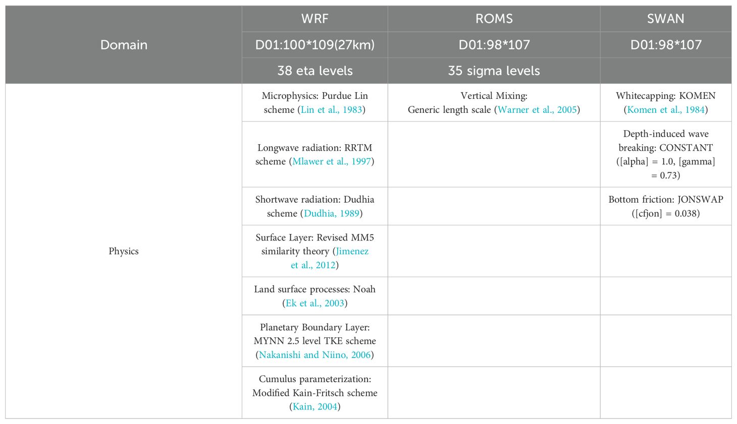
Table 1. Primary experimental setup and configuration summary for the three component models.

Two primary methods currently exist for calculating Stokes drift. One approach uses wave spectra to calculate Stokes drift (Breivik et al., 2014), while the other uses Hs, period, and wavenumber. In this study, the second method was adopted for calculating Stokes drift. The second method was chosen for its simplicity and practicality, allowing for easier implementation using Hs, wave period, and wavenumber. This approach is also consistent with previous studies, where it has been widely used to model Stokes drift and provides a reasonable approximation. Given the large-scale nature of this study, a simplified approach was preferred to ensure computational efficiency without sacrificing significant accuracy. The vertical influence of Stokes drift reaches a maximum depth, referred to as the depth of influence. When the water depth exceeds this influence depth, Stokes drift and its effects become negligible. The equation is as follows:

$\begin{array}{ll}{d}_s=\frac{1}{2k}& (1)\end{array}$

$\begin{array}{ll}k=\frac{2\pi }{\lambda }& (2)\end{array}$

$\begin{array}{ll}\lambda =cT& (3)\end{array}$

$\begin{array}{ll}c=\frac{gT}{2\pi }& (4)\end{array}$

where $d_s$ represents the depth of influence of Stokes drift; $k$ is the wave number; $\lambda$ is the wavelength; $c$ is the phase velocity; $T$ is the wave period.

For a monochromatic deep-water gravity wave under conditions of homogeneous and irrotational flow, Stokes drift is expressed by the following equation:

$\begin{array}{ll}{\overrightarrow{u}}_{\text{st}}(z)={\overrightarrow{U}}_s\exp \left(\frac{z}{d_s}\right)& (5)\end{array}$

where ${\overrightarrow{u}}_{st}$represents wave-induced Stokes drift velocity; ${\overrightarrow{U}}_s\text{ represents}$ the surface Stokes drift velocity; $z$ represents depth; d_s represents the depth of Stokes influence. During the influence of Super Typhoon Doksuri, the large typhoon waves triggered significant Stokes drift. Assuming the fluid is irrotational and inviscid, Stokes drift velocity can be determined using Equation 5.

The movement of water particles driven by Stokes drift is known as Stokes transport, which is essential for mass and energy exchange in the upper ocean. Classical coastal hydrodynamics theory suggests that greater Hs and shorter wave periods lead to enhanced mass transport via Stokes drift. Stokes transport is determined by vertically integrating Stokes drift, as represented by the following equation:

$\begin{array}{ll}{T}_{\text{s}}={\int }_{-d_s}^0{\overrightarrow{u}}_{st}(z)dz=\pi \frac{a^2}{T}& (6)\end{array}$

where $T_s$ represents Stokes transport; ${\overrightarrow{u}}_{st}$ represents Stokes drift.

Stokes transport facilitates the mass and energy transfer in the upper ocean, playing a significant role in global ocean transport processes. To compare the magnitude of Stokes transport with total transport (McWilliams and Restrepo, 1999), the Ekman-Stokes number (Es) is defined, which represents the proportion of Stokes transport to net Ekman transport. The specific equation is as follows:

$\begin{array}{ll}{E}_{\text{s}}=\frac{\left|\overrightarrow{T_{\text{s}}}\right|}{\left|\overrightarrow{T_{\text{E}}}\right|}=0.39\frac{f{U}_{10}}{C_{\text{D}}}{(1+\frac{C_{\text{D}}^{1/2}\ln 1.95}{\kappa })}^3& (7)\end{array}$

where ${\overrightarrow{T}}_E$ represents net Ekman transport; ${\overrightarrow{T}}_s=\frac{\tau }{{\rho }_{w}f}$, τ represents wind stress magnitude; ${\rho }_w$ represents seawater density; $f$ represents the Coriolis parameter; $U_{10}$ represents the wind speed at 10 m above sea level; $\kappa$ is the von Karman constant, set at 0.4; $C_D$ is the drag coefficient (Wu, 1980):

$\begin{array}{ll}{C}_D=(0.8+0.065U_{10})\times {10}^{-3}& (8)\end{array}$

3 Validation

3.1 Typhoon simulation validation

Since the typhoon eye is not directly provided by the model output, the typhoon track was determined by locating the lowest surface pressure at each simulation step. The resulting track was then compared with observations from the CMA (Figure 1). A further comparison of typhoon tracks from CMA best track data, WRF, COAWST, and ERA5 (Figure 2) revealed that the model tracks closely followed the CMA best track, with mean absolute errors (MAEs) of 61.94 km for WRF, 69.77 km for COAWST, and 29.98 km for ERA5. Errors in the tropical cyclone (TC) center were mainly observed at turning points and near landfall, likely due to the influence of complex terrain. Although the ERA5 tracks were generally consistent with observations, significant discrepancies were noted in maximum 10 m wind speed (MWS) and minimum sea level pressure (MSLP) between ERA5 and CMA best track data (Figures 2A, B). The WRF model, driven by FNL data and lacking ocean feedback, tended to overestimate TC intensity. In contrast, COAWST, which incorporated an ocean model to account for ocean feedback, provided intensity estimates that aligned more closely with CMA observations, particularly in MWS and MSLP during the steady-state phase.

Figure 1

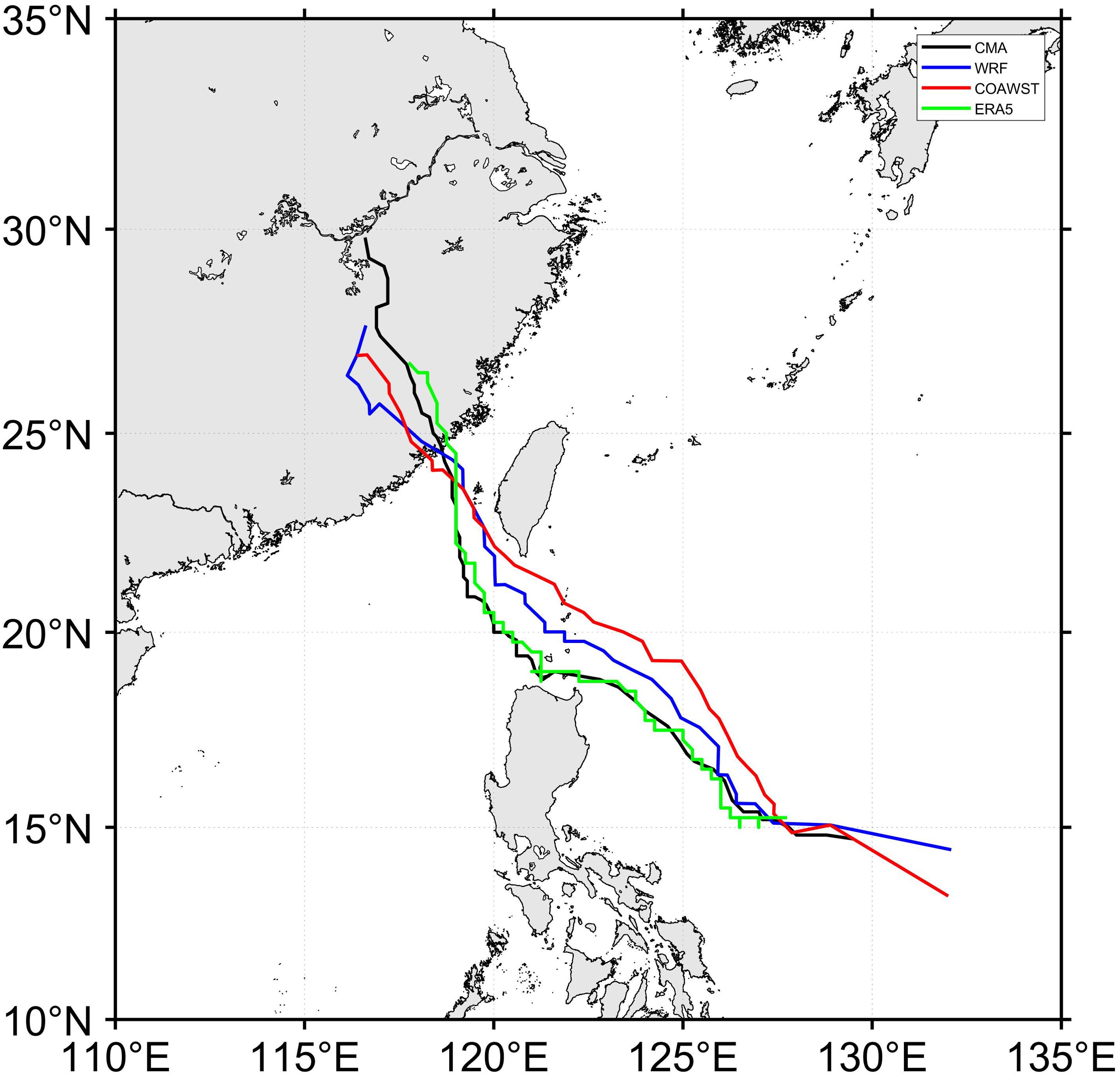
Figure 1. Track comparison for Typhoon Doksuri.

Figure 2

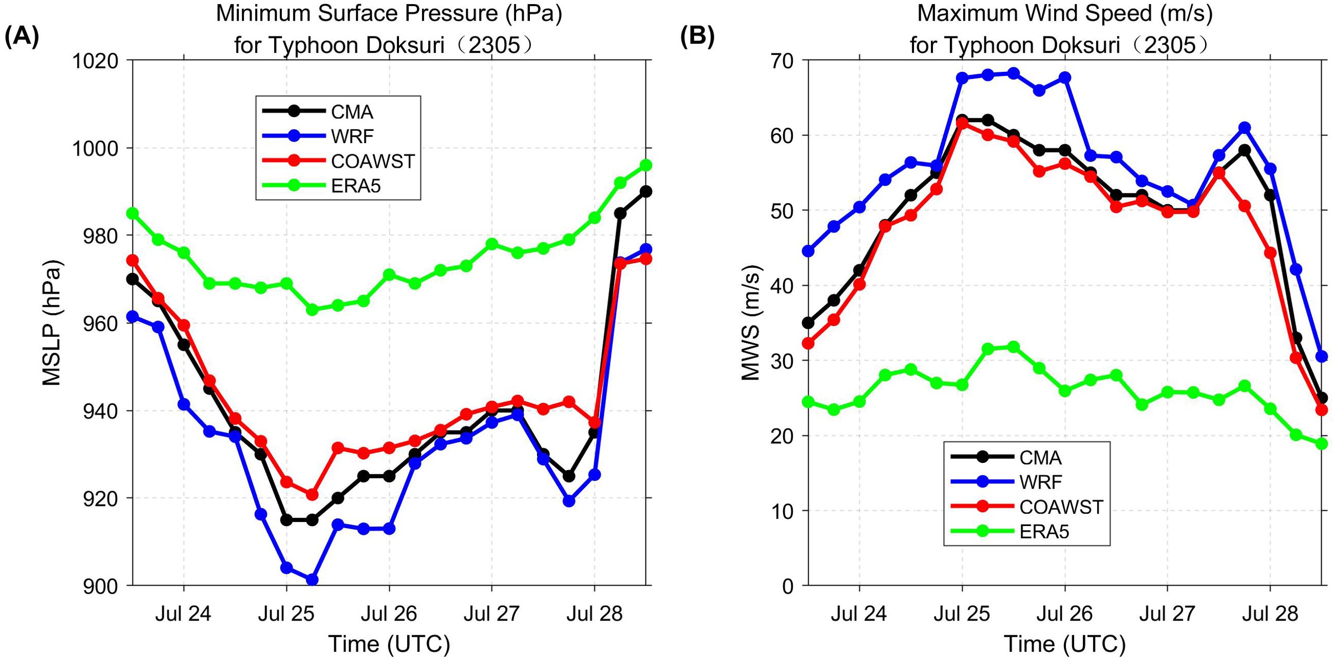
Figure 2. (A) the MSLP (hPa) and (B) the MWS (m/s) from 12 UTC 23 July to 12 UTC 28 July 2023. Results based on CMA best-track data are shown in black, with simulation results for WRF, COAWST, and ERA5 displayed in blue, green, and red, respectively.

Table 2 presents the comparative analysis of the simulated MSLP for Typhoon Doksuri. The results show that the mean MSLP error and the RMSE of MSLP were reduced in the COAWST scheme compared to ERA5 and WRF. Specifically, the RMSE of wind speed decreased by 80.06% and 16.18%, respectively, and was reduced to 7.41 hPa. The COAWST simulation showed a strong correlation with the observed MSLP, with a coefficient of 0.97.

Table 2

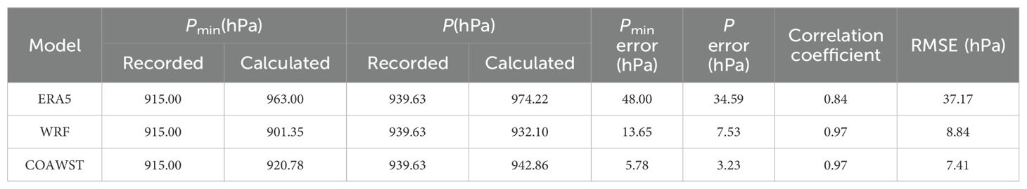
Table 2. MSLP simulation and CMA recorded values.

As shown in Table 3, during Typhoon Doksuri, the COAWST scheme reduced the mean error and RMSE of MWS compared to ERA5 and WRF, with RMSE decreases of 90.97% and 61.09%, respectively, resulting in an RMSE of 1.71 m/s. During the typhoon’s development phase, the COAWST model achieved the highest correlation with CMA recorded wind speeds, with a coefficient of 0.98, indicating that COAWST more accurately captures wind speed distribution in the typhoon’s core region.

Table 3

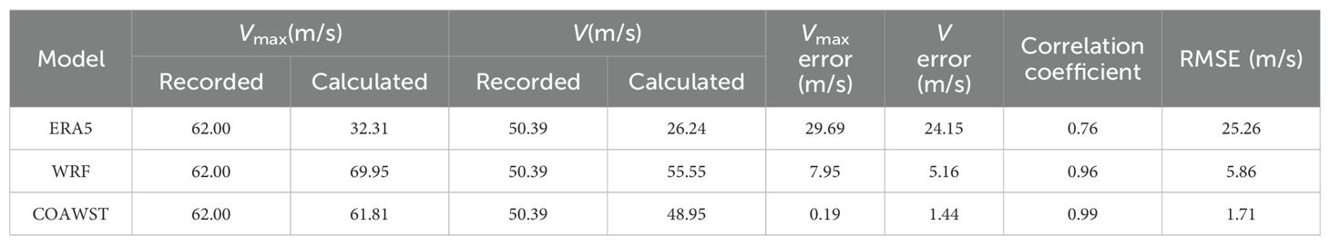
Table 3. MWS simulation and CMA recorded values.

3.2 Wave simulation validation

Surface waves are generated and developed under the influence of surface winds. Meanwhile, wave conditions can alter the current characteristics at the air-sea exchange interface (Liu et al., 2012). The simulated wave results are validated and discussed based on Hs.

To validate the wave model, wave data from the Jason-3 satellite altimeter in the Ku band were compared with ERA5 reanalysis data and the model results. The satellite track through the East China Sea (12 UTC 23 July to 12 UTC 28 July) showed the sub-satellite point pattern of the Jason-3 satellite (Figure 3). During this period, the Hs measured by the Jason-3 satellite altimeter reached up to 15.66 m, demonstrating that the altimeter effectively captured typhoon-related data.

Figure 3

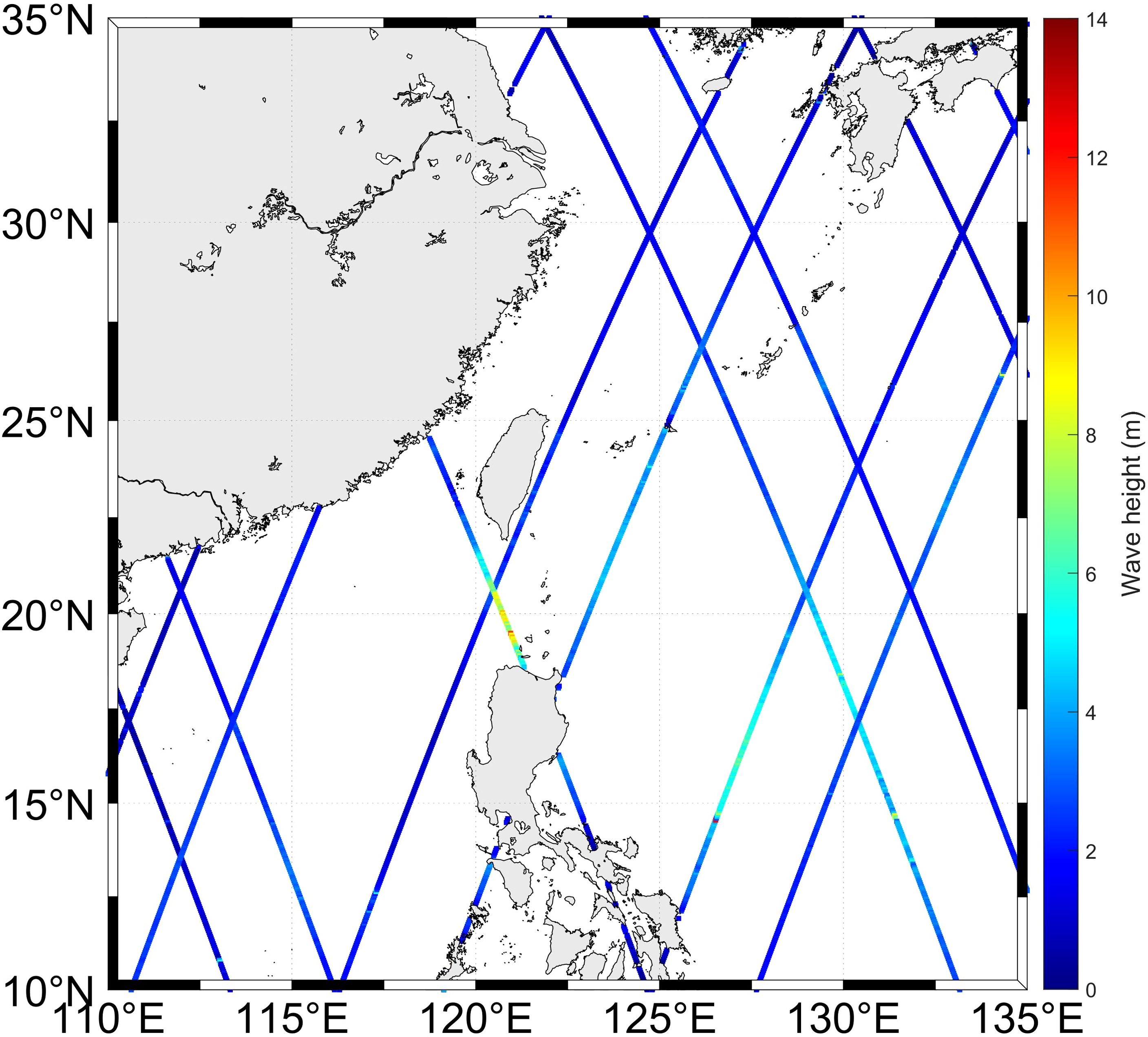
Figure 3. Hs from Jason-3.

The correlation coefficient for wave direction is above 90%, and the RMSE of the COAWST model is the smallest, below 20 degrees, indicating high accuracy in wave direction simulation.

Using a Taylor diagram, the correlation coefficient, centered RMSE and standard deviation were used to statistically compare the Hs results from ERA5 data, SWAN model, and COAWST model with Jason-3 satellite observations (Figure 4). The correlation coefficients between the model data and Jason-3 data were generally greater than 0.7, with COAWST data showing the best performance. For centered RMSE, the values ranged from 0.4 to 0.8, with COAWST having the lowest value. COAWST also performed the best in capturing the observed variability in standard deviation, with a value of approximately 0.75.

Figure 4

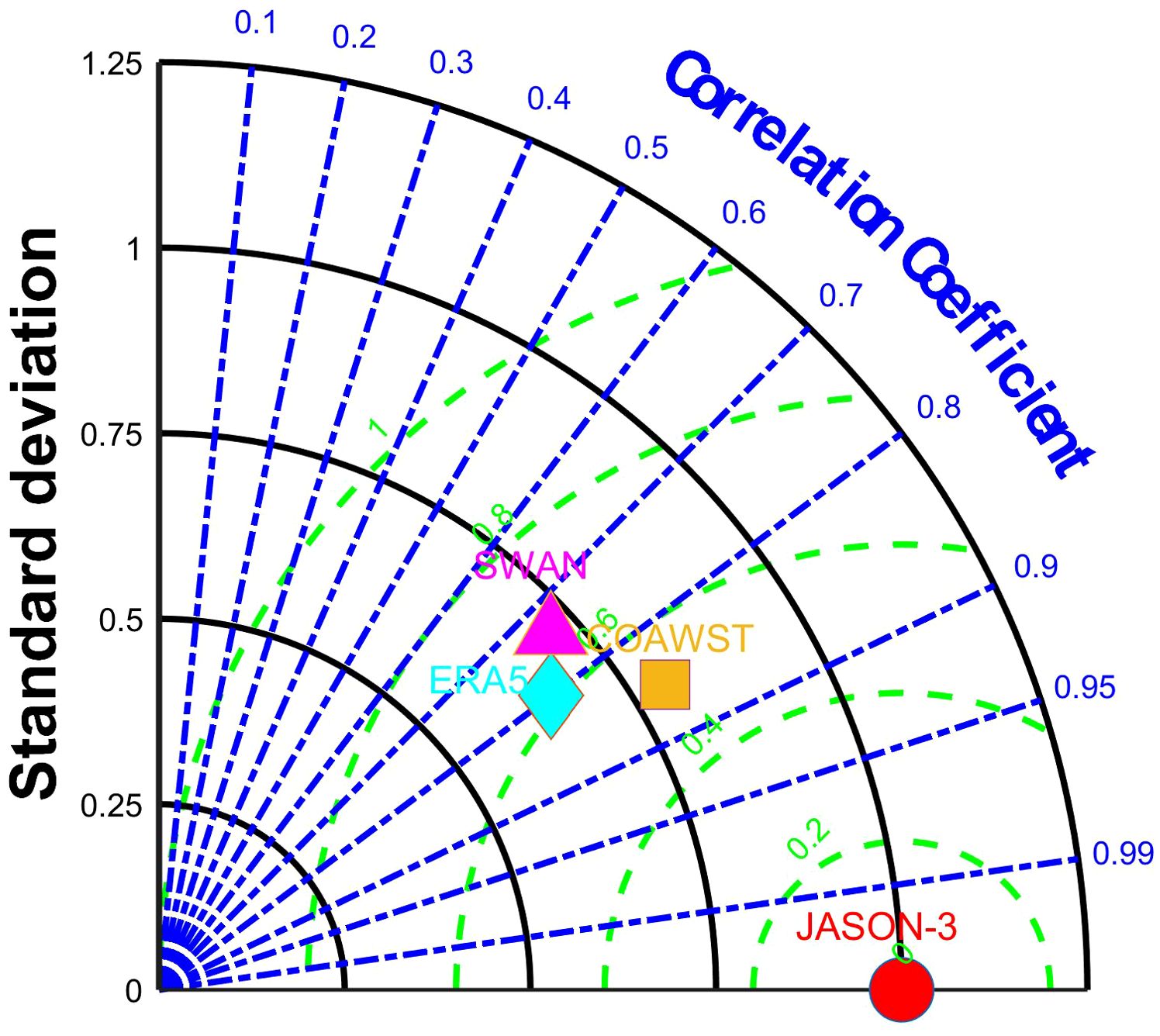
Figure 4. Taylor diagram comparing the observations with three calculated results for Hs. Green contour lines indicate the normalized centered RMSE, black contour lines show the normalized standard deviations, and the point’s azimuthal position represents the correlation coefficient between the model and JASON-3 data.

Table 4 summarizes the statistical metrics comparing JASON-3 observations with the simulation data. Among the models, the COAWST model showed the best performance, with a MAE of 0.41 m, RMSE of 0.66 m, and a correlation coefficient of 0.86 between the COAWST simulation and JASON-3 observations. These results indicate that the COAWST model provides the most accurate Hs simulation compared to other datasets.

Table 4

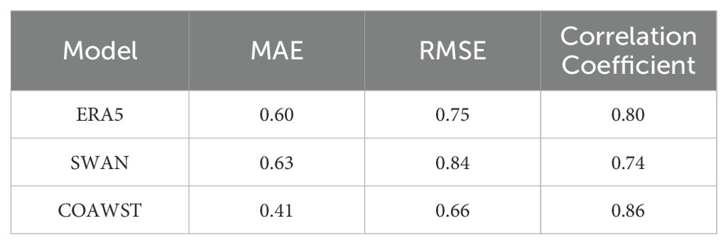
Table 4. MAE (m), RMSE (m) and correlation coefficient(R) for the JASON-3 with simulation results for Hs.

4 Results

4.1 Wind field

The wind fields at 00 UTC on July 26, 2023, capture Typhoon Doksuri at its peak intensity (Figures 5A–C). The wind speed outputs from COAWST, WRF, and ERA5 reanalysis datasets depict the structure and intensity of the typhoon at the same time step. Notably, the COAWST model provided a balanced representation of spatial extent and wind intensity, with wind speeds reaching 30 m/s over a wide area. This indicates that COAWST is particularly effective at capturing the broader impact area of the storm while maintaining reasonable accuracy in the core intensity.

Figure 5

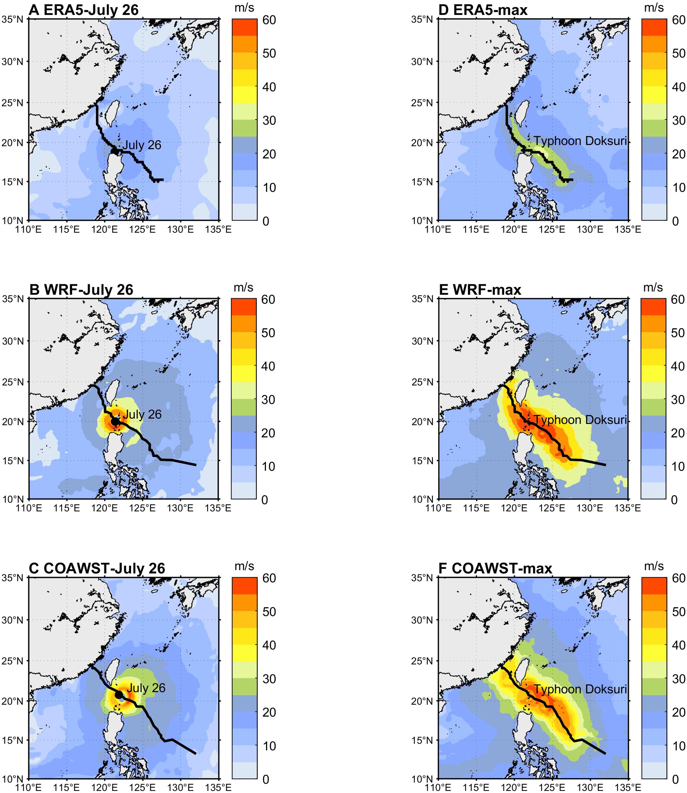
Figure 5. Wind fields of Typhoon Doksuri at 00 UTC on July 26, 2023: (A) ERA5, (B) WRF, (C) COAWST; Distribution maps of the maximum wind speed field of Typhoon Doksuri: (D) ERA5, (E) WRF, (F) COAWST.

In comparison, the WRF model, while providing a more localized and intense depiction with wind speeds exceeding 60 m/s near the core, overestimated the storm’s intensity at the expense of spatial coverage. On the other hand, ERA5 underestimated the core intensity, smoothing out important small-scale features. COAWST achieved an effective balance by integrating oceanic and atmospheric processes.

Figures 5D–F display the maximum wind speed fields across all times during Typhoon Doksuri. The fields from all three models exhibit an asymmetric distribution around the typhoon’s track, diffusing outward from the symmetric core region. The ERA5 wind field has a smaller distribution area for high wind speeds, with pronounced asymmetry (Figure 5D). The WRF-simulated wind field has the largest distribution of high wind speeds, but weaker asymmetry and a smaller wind speed gradient (Figure 5E). The COAWST-simulated wind field shows a wide distribution of high wind speeds, with prominent asymmetry and a larger wind speed gradient (Figure 5F). The maximum wind speed zone is primarily situated on the right side of the typhoon track, providing a balanced representation of spatial extent and intensity, which is particularly important for analyzing coastal impacts.

4.2 Wave field

To illustrate the impact of the distribution patterns of three different wave fields, the time 00 UTC on July 26, 2023, is selected as it represents a period with pronounced wave field characteristics (Figures 6A–C). The simulation results show that the wave field during typhoon movement exhibited a clear asymmetric characteristic, with the highest Hs in the northeastern quadrant and the lowest in the southwestern quadrant.

Figure 6

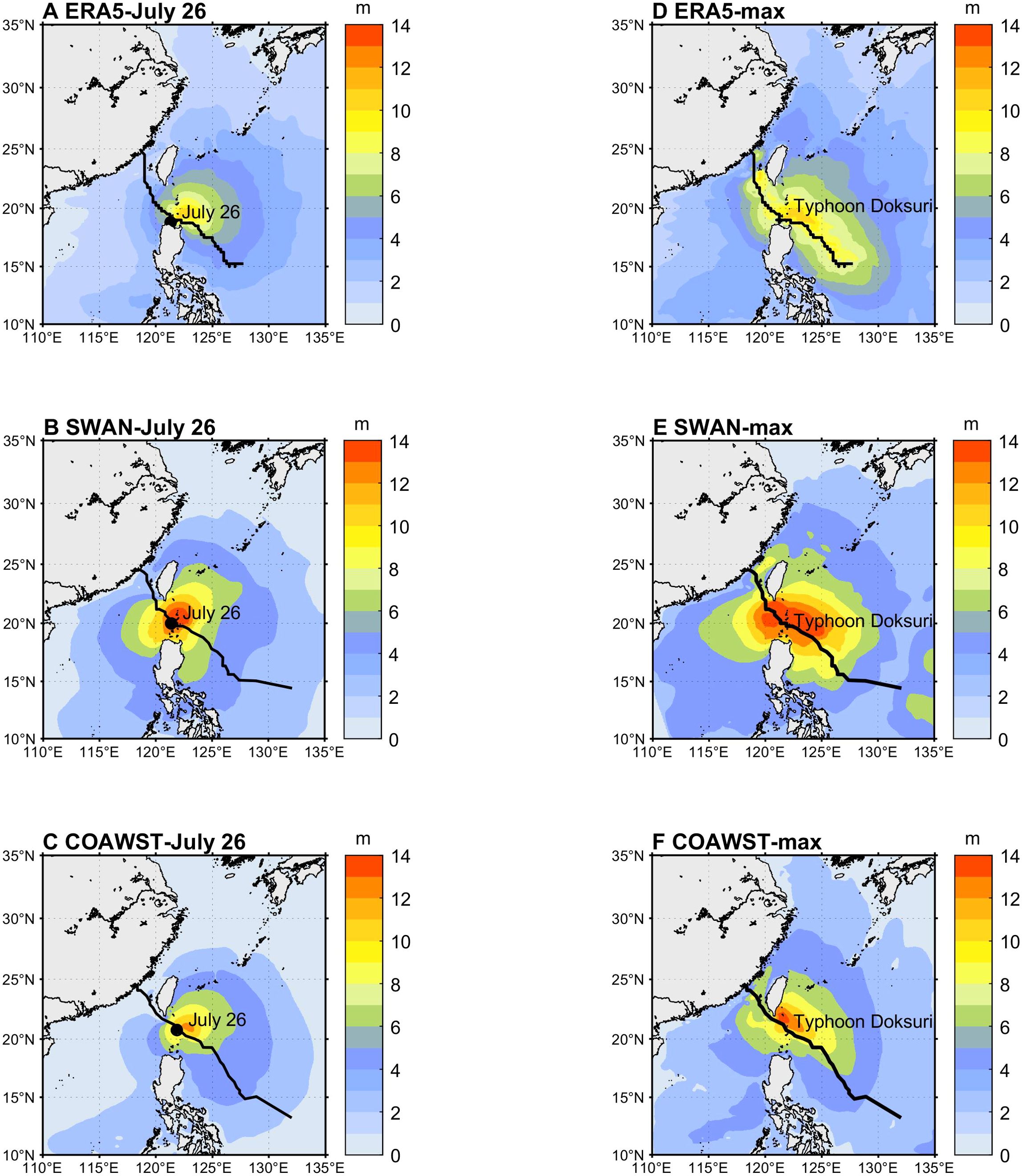
Figure 6. Wave fields of Typhoon Doksuri at 00 UTC on July 26, 2023: (A) ERA5, (B) SWAN, (C) COAWST; Distribution maps of the maximum Hs field of Typhoon Doksuri: (D) ERA5, (E) SWAN, (F) COAWST.

To explore the distribution characteristics and impact range of wave fields simulated by different models, Figures 6D–F illustrate maximum Hs fields during Typhoon Doksuri. For the maximum Hs field, all three models exhibited an asymmetric distribution centered around the typhoon track. The COAWST model exhibited the strongest asymmetry, with the maximum Hs on the right side of the typhoon track approximately 2.5 m higher than on the left, and high Hs concentrated on the first quadrant (Figure 6F). In the SWAN model (Figure 6E), the right-side maximum Hs was about 1.5 m higher, with the largest high-wave area. The ERA5 data showed a generally consistent asymmetric banded distribution, with the right-side maximum about 1 m higher than the left (Figure 6D), though overall Hs were lower and less distinct, aligning with wind field data and lower than observed values. Thus, the COAWST model demonstrated more pronounced asymmetry in maximum Hs compared to the other two models.

Additionally, from Figures 6E, F, it is evident that the maximum Hs gradient along the typhoon track in the COAWST model was smaller compared to the WRF model, indicating a slower and more gradual increase in maximum Hs, with the peak Hs occurring later. The coupled ocean-atmosphere feedback resulted in a decrease in sea surface temperature, increased atmospheric pressure, and reduced wind-wave forcing in the COAWST model, making it more consistent with real-world conditions. Due to the coupling effects, the typhoon intensity in the COAWST model was lower than that in the WRF model driving SWAN unidirectionally, leading to a lower simulated maximum Hs in the COAWST model, which was closer to the Jason-3 satellite observations.

4.3 Stokes drift

4.3.1 Stokes drift velocity

Verification and analysis of wind and wave field simulation accuracy confirm the reliability of COAWST in simulating Stokes drift. Stokes drift velocity characteristics under typhoon conditions are analyzed at four typical times (Figures 7A–D). In the early stage of typhoon formation (Figure 7A), low wind and wave intensities resulted in a Stokes drift of about 0.35 m/s. As waves intensified (Figure 7B), Stokes drift increased, showing a rightward bias with a maximum near the typhoon center, reaching 0.67 m/s in crescent-shaped contours along the right of the path. The drift field’s vortex structure also intensified, indicating strong wave energy transfer. Due to Taiwan Island’s obstruction (Figure 7C), the vortex structure fragmented, with Stokes drift peaking at 0.73 m/s southeast of the island and extending over a larger area. Before landfall (Figure 7D), Stokes drift decreased to about 0.4 m/s, while areas outside the typhoon’s influence had minimal drift, around 0.1 m/s or less. Under typhoon conditions, Stokes drift is markedly enhanced relative to non-typhoon conditions.

Figure 7

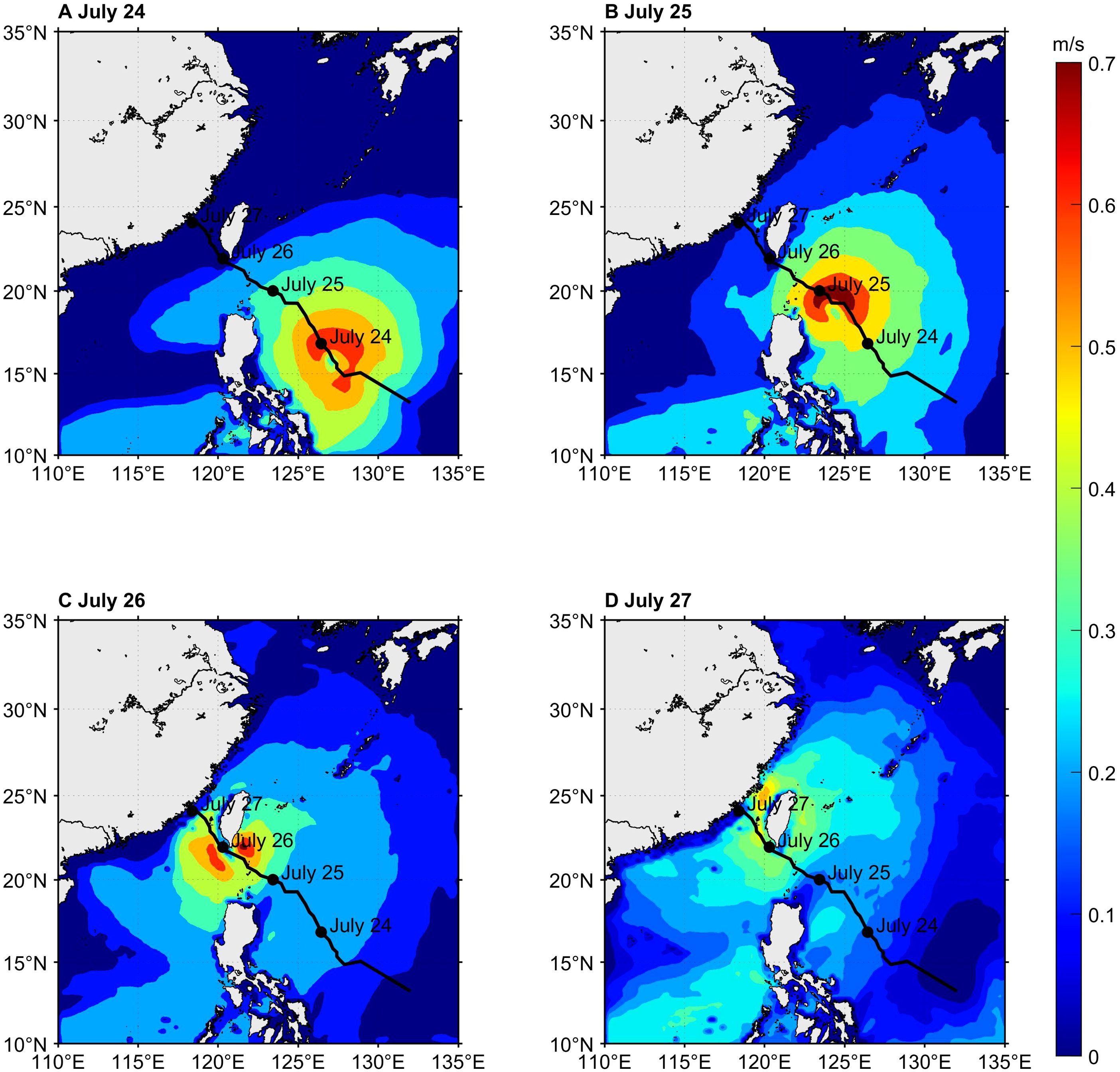
Figure 7. Distributions of the Stokes drift velocity at 12 UTC on (A) July 24, (B) July 25, (C) July 26, and (D) July 27, 2023.

These results show that Stokes drift velocity changes significantly with the movement and intensity of the typhoon, especially in the intense core region where it peaks, enhancing surface material drift in the ocean. Stokes drift distribution is generally positively correlated with wind field intensity and Hs: stronger wind increases energy input, Hs, and wavelength, intensifying wave asymmetry and Stokes drift. This causes peak Stokes drift near the typhoon center. The spatiotemporal variation of Stokes drift velocity, influenced by typhoon-induced wave asymmetry, exhibits a rightward bias with crescent-shaped contours, reflecting the nonlinear wave characteristics and net drift effect.

4.3.2 EOF analysis of stokes drift velocity

EOF decomposition of Stokes drift velocity further analyzes the spatiotemporal distribution of Stokes drift (Figures 8A–D). The first spatial pattern (EOF1) represents an average field characteristic, showing the primary spatial distribution pattern, with the corresponding temporal mode time coefficients generally matching the periods of Stokes drift velocity enhancement or reduction. EOF1 indicates that Stokes drift in this region shows significant spatial non-uniformity under the influence of the typhoon (Figure 8A), explaining 62.40% of the total variance. EOF1 of the entire Stokes drift velocity field is positive, suggesting that wave energy during the typhoon tends to concentrate in specific areas. The values are relatively highest in the southeastern Taiwan sea and coastal areas of mainland China, ranging from approximately 0.15 to 0.2, indicating a significant impact from the typhoon.

Figure 8

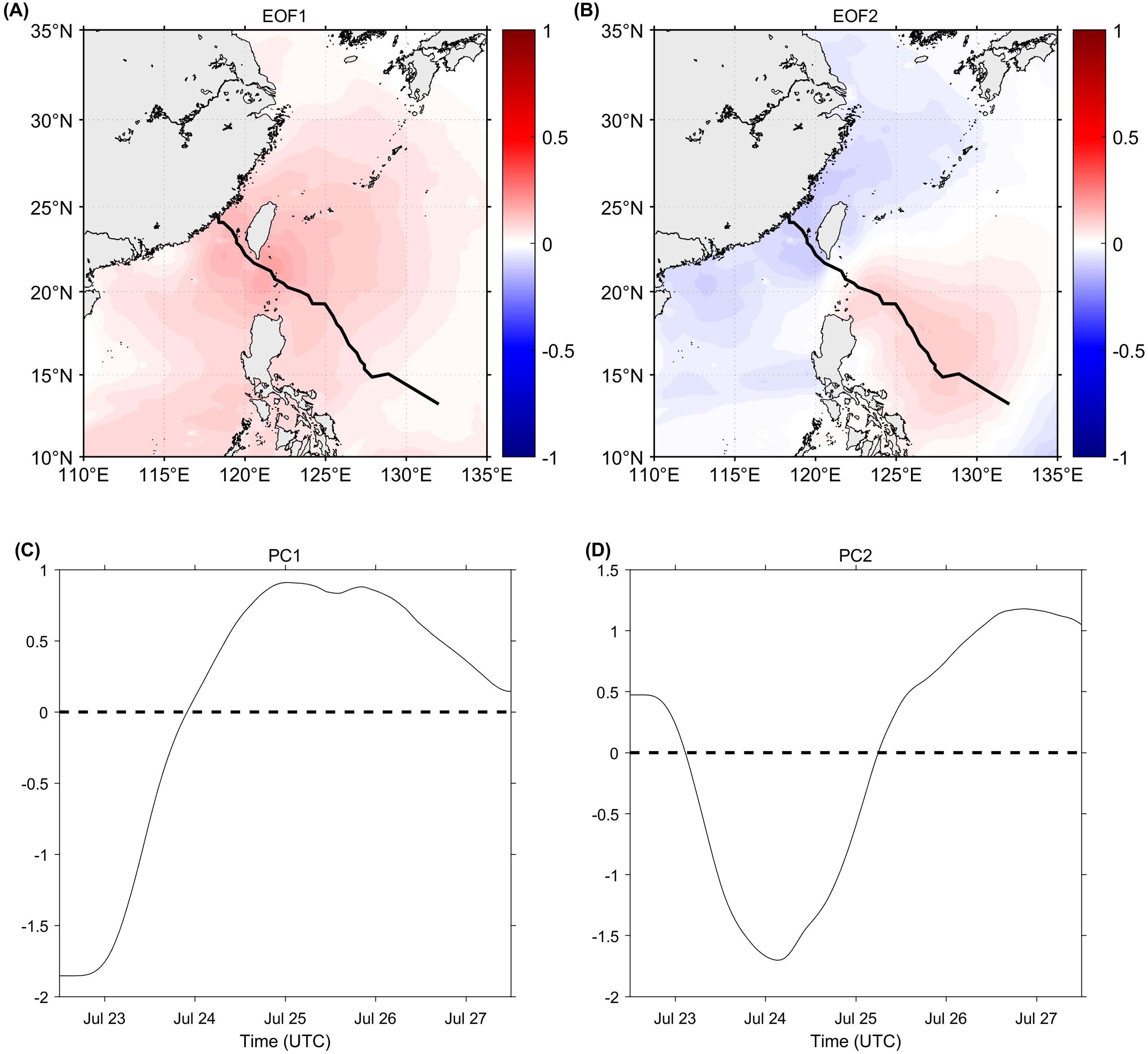
Figure 8. EOFs (left panel) and PCs (right panel) of Stokes drift velocity during Typhoon Doksuri. (A) EOF1, (B) EOF2, (C) PC1, and (D) PC2 of Stokes drift velocity during Typhoon Doksuri.

The first principal component (PC1) starts with a rapid increase from a large negative value (around -2), reaching a peak (approximately 1), and then gradually decreases, stabilizing around zero (Figure 8C). The trend of the temporal mode reflects the temporal variation of the typhoon’s impact on Stokes drift velocity in the study area. The rapid increase phase of the curve corresponds to the strengthening of the typhoon, while the plateau phase corresponds to the peak stage of the typhoon. The subsequent decrease indicates a weakening of the typhoon’s influence, with the drift velocity gradually returning to normal levels.

Combining PC1 with EOF1 allows for an analysis of Stokes drift velocity under typhoon conditions. At the onset of the typhoon, the PC1 is negative, indicating that the corresponding Stokes drift velocity at these moments is in an opposite phase to the spatial mode associated with the temporal coefficient at these times, with a generally lower Stokes drift velocity across the field. Over time, as the typhoon’s impact reaches the sea area near Taiwan, PC1 rapidly rises to a peak, corresponding to the positive center near Taiwan. When PC1 declines again, it indicates that the typhoon has moved away, and the Stokes drift velocity across the study area gradually returns to near-normal levels.

Figure 8B displays the second spatial pattern (EOF2) of the EOF analysis of Stokes drift velocity under typhoon conditions, which accounts for 25.64% of the total variance. EOF2 represents the primary pattern of temporal changes in Stokes drift velocity, rapidly progressing from southeast to northwest roughly along the typhoon path, it first increases and then decreases. The increasing (red) regions are mainly distributed in the northwestern Pacific east of the Philippines, while the decreasing (blue) regions are concentrated in the South China Sea and East China Sea. The increasing and decreasing regions exhibit a northwest-southeast directional distribution. As the typhoon progresses, the wind field distribution typically generates different wind stresses along both sides of the track, leading to an asymmetric distribution of Stokes drift velocity in the ocean surface layer. Topographic differences lead to significant variations in Stokes drift response across these regions. The terrain and current characteristics between Taiwan Island and Luzon Island may also modulate the distribution of Stokes drift velocity, such as the weakening of Stokes drift velocity in coastal areas due to the blocking effect of terrain.

The second principal component (PC2) is shown in Figure 8D. Combined with EOF2, the second mode is positively correlated with the overall Stokes drift velocity at the beginning and end phases, while it is negatively correlated at the intermediate times.

The first and second modes account for 88.04% of all the modes. The first mode primarily reflects the overall impact of the typhoon on Stokes drift velocity across the field, while the second mode captures the asymmetric changes across both sides of the typhoon track as well as the dynamic temporal evolution of drift velocity. Further analysis of EOF modes for different years and seasons could help distinguish the varied impacts of typhoons on Stokes drift in this region under different conditions.

4.3.3 Stokes transport

Stokes drift drives transport phenomena, playing a crucial role in mass and energy exchange in the upper ocean. Stokes transport during the typhoon, calculated using Equation 6, is shown in Figure 9. Consistent with the Stokes drift distribution in Figure 7, high-value areas of Stokes transport align with those of drift, mainly along the typhoon track with the maximum on the right side. Stronger wind and wave fields lead to greater Stokes drift, enhancing mass and energy transport. In the early typhoon stage (Figure 9A), Stokes drift and transport are relatively weak, around 0.2 m²/s. As typhoon intensity increases (Figure 9B), Stokes transport intensifies, reaching 5-6 m²/s near the typhoon eye with a distinct crescent-shaped structure, indicating significant wave energy within the strong wind region. During northward movement (Figure 9C), transport further increases to 10-13 m²/s, concentrated in the central and northern sea areas, driven by higher wind speeds and Hs. Upon landfall, Stokes transport weakens, with peak values reduced to 5-6 m²/s in the Taiwan Strait, reflecting the typhoon’s decline and decreasing wind and wave forces.

Figure 9

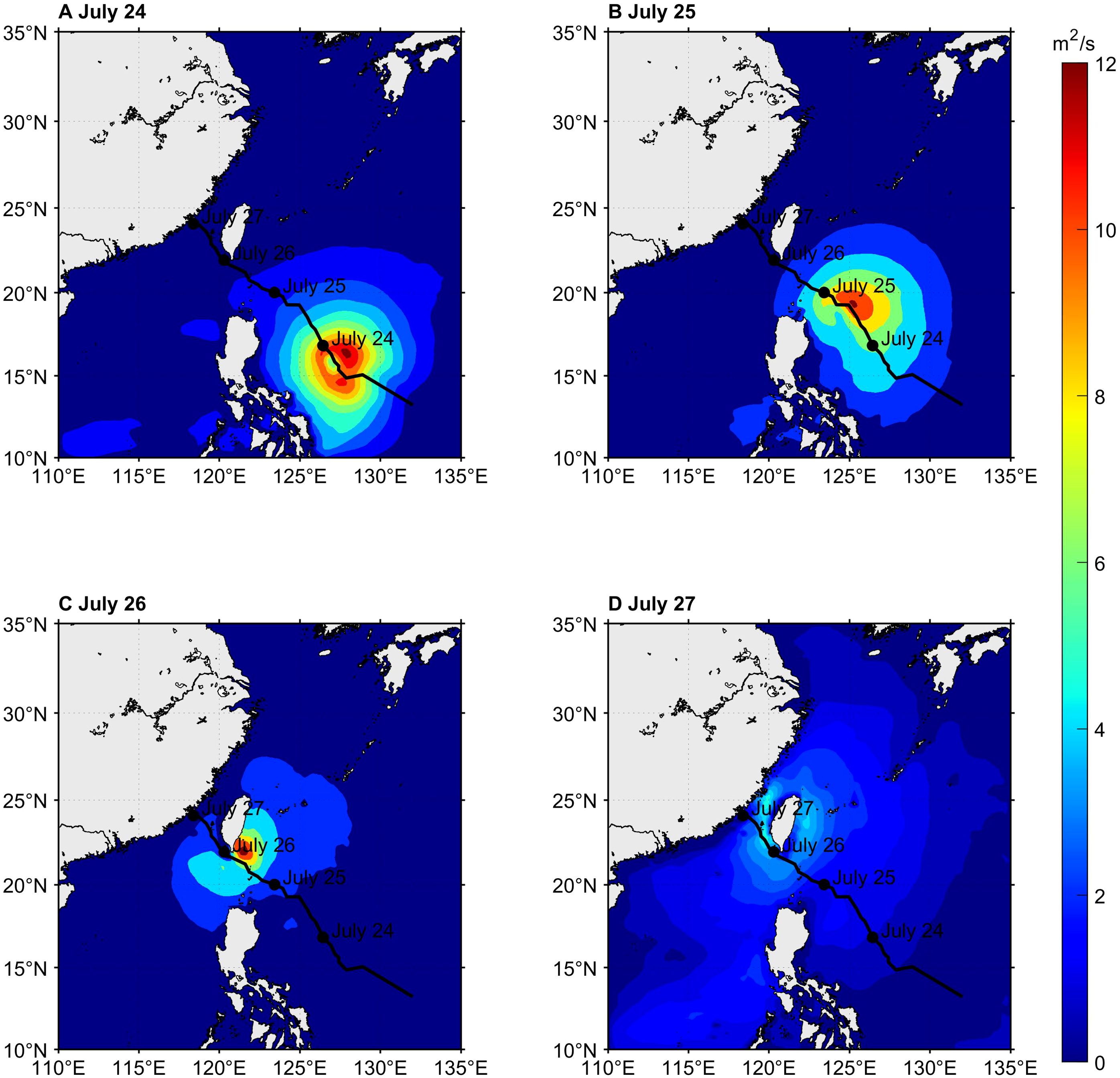
Figure 9. Distributions of the Stokes transport at 12 UTC on (A) July 24, (B) July 25, (C) July 26, and (D) July 27, 2023.

These phenomena are primarily driven by the strong impact of the typhoon wind field on ocean waves. During intensification, high waves from strong winds greatly increased Stokes transport intensity. Wind fields asymmetry and water particle movement created a distinct spatial pattern of Stokes transport along the typhoon track. As the typhoon weakened, decreasing wind and wave strength led to a reduction in Stokes transport intensity.

In ocean regions with strong currents below the surface, the shear effect of the current may have a significant impact on Stokes drift and the associated mass transport. In the case of shear flow propagating obliquely to the wave direction, the maximum induced mass transport no longer occurs at the still water surface but at a certain depth below (Li et al., 2024). The shear of the current can alter momentum transfer and vortex structures between water layers, thus affecting the spatial distribution and intensity of Stokes drift. Particularly under extreme weather conditions, such as typhoons, the interaction between currents and wind-waves may lead to significant ocean dynamic effects in localized areas, thereby altering the transport processes of matter and energy. Therefore, further consideration of the vertical shear effects of currents is crucial for improving the accuracy and predictive capability of Stokes drift models, especially in ocean regions with complex flow fields.

4.3.4 Stokes drift depth

The influence depth of Stokes drift during Typhoon Doksuri, calculated from Equation 1 and displayed in Figure 10, reflects the spatial distribution of Stokes drift, emphasizing dynamic changes as the typhoon traversed sea areas. In the early stage (Figure 10A), Stokes drift depth was relatively shallow and uniformly distributed, reflecting weaker wind field impacts on the surface layer. In the mid-stage (Figure 10B), depth increased significantly, especially in the right-front (northeastern) region, due to enhanced wind speed and pressure gradients. At the peak stage (Figure 10C), Stokes drift depth reached its maximum, exceeding 20 m, around the typhoon center, indicating intense wave energy transfer and vertical mixing over a broader area. In the late stage (Figure 10D), drift depth decreased, as the influence of wind waves and currents weakened. These results show that Stokes drift depth varies significantly with typhoon intensity and position, particularly in the core region, promoting mass and energy exchange, enhancing vertical turbulence, and cooling the upper ocean, thus improving the realism of typhoon simulations.

Figure 10

Figure 10. Distributions of the Stokes drift depth at 12 UTC on (A) July 24, (B) July 25, (C) July 26, and (D) July 27, 2023.

4.3.5 Ekman-stokes number

To investigate the variation of the Ekman-Stokes number during the typhoon process, the analysis was conducted based on the track of Typhoon Doksuri, focusing on the changes of the Ekman-Stokes number along the latitude of the typhoon track. The Ekman-Stokes number at typical times was calculated using Equation 7, as shown in Figure 11. From the analysis of the Ekman-Stokes number (Figures 11A–D), it can be observed that it exhibited significant fluctuations across different latitudinal ranges over time. As the dates progressed, the Ekman-Stokes number generally showed an increasing and then decreasing trend in the north-south direction (latitude range 15°N to 25°N).

Figure 11

Figure 11. Distributions of the Ekman-Stokes number at 12 UTC on (A) July 24, (B) July 25, (C) July 26, and (D) July 27, 2023.

Overall, the Ekman-Stokes number decreases sharply with increasing latitude, primarily due to the enhancement of the Coriolis force at higher latitudes, which significantly strengthens the Ekman flow, while the Stokes drift becomes relatively weaker. The relative interplay between these two factors results in the observed sharp decline of the Ekman-Stokes number with increasing latitude.

From July 24 to July 26, the latitude of the first minimum in each figure corresponds to the location of the typhoon’s high-value area at that time, with significant peaks on both sides indicating strong Stokes transport. Subsequently, the Ekman-Stokes number decreases along the latitude. In the early stages of the typhoon at lower latitudes, Stokes transport comprises approximately 27% of the net transport. As the typhoon grows and moves, the proportion of Stokes transport gradually increases. On July 27, in the region from 22°N to 24°N, the Ekman-Stokes number reaches its peak (close to 0.35). Throughout the typhoon’s passage, Stokes drift remains relatively weak at lower latitudes, while wave contributions in higher latitude areas gradually intensify.

5 Discussion and conclusion

This study utilized the COAWST model to simulate the wind field, wave field, and Stokes drift during Typhoon Doksuri, revealing the typhoon’s impact on the surface ocean dynamics from the perspectives of wind, wave, and Stokes drift.

Using the COAWST coupled model, coarse-grid simulations of wind speed and spatial distribution during the typhoon were conducted. The peak wind speed had an RMSE of only 1.71 m/s compared to observations, with a peak wind speed reaching 61.81 m/s. The wind field exhibited significant asymmetry, especially in the first quadrant around the typhoon center, where wind speeds were stronger. Compared to using only WRF or ERA5 reanalysis data, the COAWST model significantly improved the accuracy of typhoon wind field simulation.

Wave field changes during the typhoon showed that the maximum Hs on both sides of the typhoon track differed by 2.5 m, with higher values on the right side, reflecting the asymmetry in wave field distribution. Wave energy rapidly increased as the typhoon passed, then gradually decayed after the typhoon moved away. The correlation between the wave field and JASON-3 satellite data was highest at 0.86, particularly in regions with the strongest wave energy, where the COAWST model’s simulation of Hs closely matched the observations.

Stokes drift exhibited significant spatial and temporal variations during the typhoon. During the typhoon’s peak, the Stokes drift velocity reached 0.73 m/s. EOF analysis showed that the first two modes explained 85% of the variance in Stokes drift and transport, revealing that the wave and drift effects in the first quadrant around the typhoon center (upper right of the typhoon track) were most significant. The first mode primarily reflected the overall influence of the typhoon on Stokes drift velocity, while the second mode captured both the asymmetric changes across the track and the dynamic temporal evolution. Further analysis could examine EOF mode plots for different years and seasons to distinguish the varied impacts of typhoons under different conditions. The Stokes transport depth reached up to 20 m, with a transport intensity of 0.73 m²/s, indicating a strong influence of waves on the upper ocean. The calculated Ekman-Stokes number showed that the contribution of Stokes drift peaked during the typhoon’s landfall stage, with local values exceeding 0.35. The characteristics of Stokes drift under typhoon conditions can be further clarified by comparing various metrics between typhoon and normal weather conditions.

This study provides an initial analysis of Stokes drift, yet certain limitations remain, highlighting directions for future research. Future work should investigate how varying typhoon types influence Stokes drift distribution, particularly in contrasting coastal and deep-sea areas. Future studies could incorporate observational data or hypothetical material fields (e.g., floating debris, plankton, oil) to examine transport dynamics and interactions with Ekman currents and eddies at different depths. Increased typhoon frequency and intensity may amplify upper-ocean material and energy transport. Future studies could explore spatial distribution changes in Stokes drift under various climate scenarios. These limitations underscore avenues for future research to enhance understanding of the dynamic role of Stokes drift in typhoon-ocean responses.

By conducting detailed simulations and analyses of wind, wave, and Stokes drift, this study revealed the complex dynamics of ocean-atmosphere-wave interactions during typhoons. The COAWST model demonstrated high simulation capability for storm surge, ocean waves, and ocean transport, providing important theoretical support and quantitative evidence for further studies on typhoon-induced ocean dynamics.

Data availability statement

The raw data supporting the conclusions of this article will be made available by the authors, without undue reservation.

Author contributions

YH: Conceptualization, Formal Analysis, Methodology, Writing – original draft, Writing – review & editing. CZ: Funding acquisition, Supervision, Writing – review & editing. ZW: Data curation, Formal Analysis, Visualization, Writing – review & editing. YW: Methodology, Validation, Writing – review & editing. CT: Methodology, Validation, Writing – review & editing. XZ: Methodology, Validation, Writing – review & editing. JZ: Data curation, Formal Analysis, Validation, Writing – review & editing.

Funding

The author(s) declare that financial support was received for the research, authorship, and/or publication of this article. This research received funding from the National Natural Science Foundation (No. 42130402, No. 42176012); and the National Key Research and Development Program (No. 2021YFC3101702).

Conflict of interest

The authors declare that the research was conducted in the absence of any commercial or financial relationships that could be construed as a potential conflict of interest.

Generative AI statement

The author(s) declare that no Generative AI was used in the creation of this manuscript.

Publisher’s note

All claims expressed in this article are solely those of the authors and do not necessarily represent those of their affiliated organizations, or those of the publisher, the editors and the reviewers. Any product that may be evaluated in this article, or claim that may be made by its manufacturer, is not guaranteed or endorsed by the publisher.

References

Booij N., Ris R. C., Holthuijsen L. H. (1999). A third-generation wave model for coastal regions: 1. Model description and validation. J. Geophys. Res. Oceans 104 (C4), 7649–7666. doi: 10.1029/98JC02622

Crossref Full Text | Google Scholar

Breivik Ø., Janssen P. A. E. M., Bidlot J.-R. (2014). Approximate stokes drift profiles in deep water. J. Phys. Oceanogr. 44, 2433–2445. doi: 10.1175/JPO-D-14-0020.1

Crossref Full Text | Google Scholar

Chen Z., Zhang C., Huang Y., Feng Y., Zhong S., Dai G., et al. (2014). Track of Super Typhoon Haiyan predicted by a typhoon model for the South China Sea. J. Meteorol. Res. 28, 510–523. doi: 10.1007/s13351-014-3269-2

Crossref Full Text | Google Scholar

Clarke A. J., Van Gorder S. (2018). The relationship of near-surface flow, stokes drift and the wind stress. J. Geophys. Research-Oceans 123, 4680–4692. doi: 10.1029/2018jc014102

Crossref Full Text | Google Scholar

Commerce, N.C.f.E.P.N.W.S.N.U.S.D.o (2015). NCEP GDAS/FNL 0.25 Degree Global Tropospheric Analyses and Forecast Grids (Boulder, CO.: Research Data Archive at the National Center for Atmospheric Research, Computational and Information Systems Laboratory). doi: 10.5065/D65Q4T4Z

Crossref Full Text | Google Scholar

Cunningham H. J., Higgins C., van den Bremer T. S. (2022). The role of the unsteady surface wave-driven Ekman-Stokes flow in the accumulation of floating marine litter. J. Geophys. Res. Oceans 127 (6), e2021JC018106. doi: 10.1029/2021jc018106

Crossref Full Text | Google Scholar

Davis C., Wang W., Chen S. S., Chen Y., Corbosiero K., DeMaria M., et al. (2008). Prediction of landfalling hurricanes with the advanced hurricane WRF model. Month. Weather Rev. 136, 1990–2005. doi: 10.1175/2007MWR2085.1

Crossref Full Text | Google Scholar

Desai S. (2016). Jason-3 GPS based orbit and SSHA OGDR (PO.DAAC, CA, USA: NASA Physical Oceanography Distributed Active Archive Center). doi: 10.5067/J3L2G-OGDRF

Crossref Full Text | Google Scholar

Dudhia J. (1989). Numerical study of convection observed during the winter monsoon experiment using a mesoscale two-dimensional model. J. Atmos. Sci. 46, 3077–3107. doi: 10.1175/1520-0469(1989)046<3077:NSOCOD>2.0.CO;2

Crossref Full Text | Google Scholar

Ek M. B., Mitchell K. E., Lin Y., Rogers E., Grunmann P., Koren V., et al. (2003). Implementation of Noah land surface model advances in the National Centers for Environmental Prediction operational mesoscale Eta model. J. Geophys. Research-Atmos. 108, 8851. doi: 10.1029/2002JD003296

Crossref Full Text | Google Scholar

Fan P., Jin J., Guo R., Li G., Zhou G. (2023). The effects of wave-induced stokes drift and mixing induced by nonbreaking surface waves on the ocean in a climate system ocean model. J. Mar. Sci. Eng. 11, 1868. doi: 10.3390/jmse11101868

Crossref Full Text | Google Scholar

Haidvogel D. B., Arango H. G., Hedstrom K., Beckmann A., Malanotte-Rizzoli P., Shchepetkin A. F. (2000). Model evaluation experiments in the North Atlantic Basin: simulations in nonlinear terrain-following coordinates. Dynam. Atmos. Oceans 32, 239–281. doi: 10.1016/S0377-0265(00)00049-X

Crossref Full Text | Google Scholar

Hsiao S.-C., Wu H.-L., Chen W.-B. (2023). Study of the optimal grid resolution and effect of wave-wave interaction during simulation of extreme waves induced by three ensuing typhoons. J. Mar. Sci. Eng. 11, 653. doi: 10.3390/jmse11030653

Crossref Full Text | Google Scholar

Inagaki N., Shibayama T., Esteban M., Takabatake T. (2020). Effect of translate speed of typhoon on wind waves. Natural Hazards 105, 841–858. doi: 10.1007/s11069-020-04339-4

Crossref Full Text | Google Scholar

Jimenez P., Dudhia J., González Rouco J. F., Navarro J., Montávez J., Garcia Bustamante E. (2012). A revised scheme for the WRF surface layer formulation. Month. Weather Rev. 140, 898–918. doi: 10.1175/MWR-D-11-00056.1

Crossref Full Text | Google Scholar

Kain J. S. (2004). The kain–fritsch convective parameterization: an update. J. Appl. Meteorol. 43, 170–181. doi: 10.1175/1520-0450(2004)043<0170:TKCPAU>2.0.CO;2

Crossref Full Text | Google Scholar

Komen G. J., Hasselmann S., Hasselmann K. (1984). On the existence of a fully developed wind-sea spectrum. J. Phys. Oceanogr. 14, 1271–1285. doi: 10.1175/1520-0485(1984)014<1271:OTEOAF>2.0.CO;2

Crossref Full Text | Google Scholar

Lee C. B., Kim J.-C., Belorid M., Zhao P. (2016). Performance evaluation of four different land surface models in WRF. Asian J. Atmos. Environ. 10, 42–50. doi: 10.5572/ajae.2016.10.1.042

Crossref Full Text | Google Scholar

Li Y., Zheng Z., Kalisch H. (2024). Stokes drift and particle trajectories induced by surface waves atop a shear flow. Front. Mar. Sci. 11. doi: 10.3389/fmars.2024.1445116

Crossref Full Text | Google Scholar

Lim Kam Sian K. T. C., Dong C., Liu H., Wu R., Zhang H. (2020). Effects of model coupling on typhoon kalmaegi, (2014) simulation in the South China sea. Atmosphere 11, 432. doi: 10.3390/atmos11040432

Crossref Full Text | Google Scholar

Lin L.-C., Wu C. H. (2021). Unexpected meteotsunamis prior to Typhoon Wipha and Typhoon Neoguri. Natural Hazards 106, 1673–1686. doi: 10.1007/s11069-020-04313-0

Crossref Full Text | Google Scholar

Lin Y.-L., Farley R. D., Orville H. D. (1983). Bulk parameterization of the snow field in a cloud model. J. Appl. Meteorol. Climatol. 22, 1065–1092. doi: 10.1175/1520-0450(1983)022<1065:BPOTSF>2.0.CO;2

Crossref Full Text | Google Scholar

Liu B., Guan C., Xie L.a., Zhao D. (2012). An investigation of the effects of wave state and sea spray on an idealized typhoon using an air-sea coupled modeling system. Adv. Atmos. Sci. 29, 391–406. doi: 10.1007/s00376-011-1059-7

Crossref Full Text | Google Scholar

Lu X., Yu H., Ying M., Zhao B., Zhang S., Lin L., et al. (2021). Western north pacific tropical cyclone database created by the China meteorological administration. Adv. Atmos. Sci. 38, 690–699. doi: 10.1007/s00376-020-0211-7

Crossref Full Text | Google Scholar

Luo C., Shang S., Xie Y., He Z., Wei G., Zhang F., et al. (2023). Evaluation of the effect of WRF physical parameterizations on typhoon and wave simulation in the Taiwan strait. Water 15, 1526. doi: 10.3390/w15081526

Crossref Full Text | Google Scholar

McWilliams J. C., Huckle E., Liang J.-H., Sullivan P. P. (2012). The wavy ekman layer: langmuir circulations, breaking waves, and Reynolds stress. J. Phys. Oceanogr. 42, 1793–1816. doi: 10.1175/jpo-d-12-07.1

Crossref Full Text | Google Scholar

McWilliams J. C., Restrepo J. M. (1999). The wave-driven ocean circulation. J. Phys. Oceanogr. 29, 2523–2540. doi: 10.1175/1520-0485(1999)029<2523:TWDOC>2.0.CO;2

Crossref Full Text | Google Scholar

Mlawer E. J., Taubman S. J., Brown P. D., Iacono M. J., Clough S. A. (1997). Radiative transfer for inhomogeneous atmospheres: RRTM, a validated correlated-k model for the longwave. J. Geophys. Research-Atmos. 102, 16663–16682. doi: 10.1029/97JD00237

Crossref Full Text | Google Scholar

Nakanishi M., Niino H. (2006). An improved Mellor–Yamada level-3 model: its numerical stability and application to a regional prediction of advection fog. Boundary-Layer Meteorol. 119, 397–407. doi: 10.1007/s10546-005-9030-8

Crossref Full Text | Google Scholar

Rabe T. J., Kukulka T., Ginis I., Hara T., Reichl B. G., D’Asaro E. A., et al. (2015). Langmuir turbulence under hurricane Gustav, (2008). J. Phys. Oceanogr. 45, 657–677. doi: 10.1175/jpo-d-14-0030.1

Crossref Full Text | Google Scholar

Sayol J. M., Orfila A., Oey L. Y. (2016). Wind induced energy-momentum distribution along the Ekman-Stokes layer. Application to the Western Mediterranean Sea climate. Deep-Sea Res. Part I-Oceanogr. Res. Papers 111, 34–49. doi: 10.1016/j.dsr.2016.01.004

Crossref Full Text | Google Scholar

Shchepetkin A. F., McWilliams J. C. (2005). The regional oceanic modeling system (ROMS): a split-explicit, free-surface, topography-following-coordinate oceanic model. Ocean Model. 9, 347–404. doi: 10.1016/j.ocemod.2004.08.002

Crossref Full Text | Google Scholar

van den Bremer T. S., Breivik O. (2018). Stokes drift. Philos. Trans. A Math Phys. Eng. Sci. 376 (2111), 20170104. doi: 10.1098/rsta.2017.0104

PubMed Abstract | Crossref Full Text | Google Scholar

Wang J., Mo D., Hou Y., Li S., Li J., Du M., et al. (2022). The impact of typhoon intensity on wave height and storm surge in the northern east China sea: A comparative case study of typhoon muifa and typhoon lekima. J. Mar. Sci. Eng. 10 (2), 192. doi: 10.3390/jmse10020192

Crossref Full Text | Google Scholar

Wang Y., Sun Y., Liao Q., Zhong Z., Hu Y., Liu K. (2017). Impact of initial storm intensity and size on the simulation of tropical cyclone track and western Pacific subtropical high extent. J. Meteorol. Res. 31, 946–954. doi: 10.1007/s13351-017-7024-3

Crossref Full Text | Google Scholar

Warner J. C., Armstrong B., He R., Zambon J. B. (2010). Development of a coupled ocean–atmosphere–wave–sediment transport (COAWST) modeling system. Ocean Model. 35, 230–244. doi: 10.1016/j.ocemod.2010.07.010

Crossref Full Text | Google Scholar

Warner J. C., Sherwood C. R., Arango H. G., Signell R. P. (2005). Performance of four turbulence closure models implemented using a generic length scale method. Ocean Model. 8, 81–113. doi: 10.1016/j.ocemod.2003.12.003

Crossref Full Text | Google Scholar

Woo H.-J., Park K.-A. (2021). Estimation of extreme significant wave height in the northwest pacific using satellite altimeter data focused on typhoons, (1992-2016). Remote Sens. 13, 1063. doi: 10.3390/rs13061063

Crossref Full Text | Google Scholar

Wu J. (1980). Wind-Stress coefficients over Sea surface near Neutral Conditions—A Revisit. J. Phys. Oceanogr. 10, 727–740. doi: 10.1175/1520-0485(1980)010<0727:WSCOSS>2.0.CO;2

Crossref Full Text | Google Scholar

Wu Y., Dou S., Fan Y., Yu S., Dai W. (2023). Research on the influential characteristics of asymmetric wind fields on typhoon waves. Front. Mar. Sci. 10. doi: 10.3389/fmars.2023.1113494

Crossref Full Text | Google Scholar

Ying M., Zhang W., Yu H., Lu X., Feng J., Fan Y., et al. (2014). An overview of the China meteorological administration tropical cyclone database. J. Atmos. Ocean. Technol. 31, 287–301. doi: 10.1175/JTECH-D-12-00119.1

Crossref Full Text | Google Scholar

Yu T., Deng Z., Zhang C., Hamdi Ali A. (2024). Detecting the role of Stokes drift under typhoon condition by a fully coupled wave-current model. Front. Mar. Sci. 11. doi: 10.3389/fmars.2024.1364960

Crossref Full Text | Google Scholar

Zhao B., Qiao F., Cavaleri L., Wang G., Bertotti L., Liu L. (2017). Sensitivity of typhoon modeling to surface waves and rainfall. J. Geophys. Research-Oceans 122, 1702–1723. doi: 10.1002/2016jc012262

Crossref Full Text | Google Scholar

Zheng M., Zhang Z., Zhang W., Fan M., Wang H. (2023). Effects of ocean states coupling on the simulated Super Typhoon Megi, (2010) in the South China Sea. Front. Mar. Sci. 10. doi: 10.3389/fmars.2023.1105687

Crossref Full Text | Google Scholar