Impacts of IOD and ENSO on the phytoplankton’s vertical variability in the Northern Indian Ocean

The Indian Ocean Dipole (IOD) and El Niño–Southern Oscillation (ENSO) are the primary climatic modes that profoundly impact physical and biological processes in the Northern Indian Ocean (NIO). IOD- and ENSO-related vertical phytoplankton anomalies, however, remain poorly understood. Using the three-dimensional Chlorophyll a concentration dataset generated by a machine learning model, this study examines IOD- and ENSO-linked vertical phytoplankton anomalies over the entire euphotic layer (0–100 m) in the NIO during 2000–2019. Results reveal that IOD and ENSO trigger significant opposite changes in phytoplankton at 0–50 m and 50–100 m. The effects of IOD and ENSO on the vertical structure of phytoplankton are generally asymmetric, with anomalies at 0–50 m being significantly larger than that at 50–100 m. During summer and fall, the significant vertical phytoplankton anomalies in the Central Arabian Sea (CAS), Southern Tip of India (STI), and the Eastern Equatorial Indian Ocean (EEIO), are primarily related to IOD forcing. IOD-linked negative (positive) phytoplankton anomalies at 0–50 m (50–100 m) are driven by the westward propagating downwelling Rossby waves. During winter and spring, due to the local wind anomalies and shallower thermocline, the Seychelles–Chagos Thermocline Ridge (SCTR) is the only region where ENSO exhibits greater positive effects on phytoplankton at 50–100 m than IOD. Different from IOD, the ENSO-related wind reversal impedes subsurface upwelling in the STI and EEIO, thereby constraining vertical biological activity. These findings could shed light on how phytoplankton will respond to changing ocean dynamics under global warming.

1 Introduction

The Northern Indian Ocean (NIO, 40°–100°E, 10°S–30°N, Figure 1) is characterized by the existence of monsoonal winds and reversing currents, due to the vast Asian landmass at low latitudes (Hermes et al., 2019). Under the complex ocean-atmosphere interaction systems, phytoplankton in the NIO exhibit a variety of three-dimensional (3-D) structures (Figure 1). Recent studies have offered remarkable insights into the potentially profound effects of climate change on phytoplankton (Currie et al., 2013; Hays et al., 2005; Hu et al., 2021; Pandey et al., 2019; Racault et al., 2017). Beyond its direct impact on local marine ecosystems, phytoplankton photosynthesis in the Indian Ocean basin may account for approximately 20% of the global oceanic uptake of anthropogenic CO₂ (Takahashi et al., 2002; Gruber et al., 2019), thereby helping to buffer the effects of global warming. As a result, the tight coupling mechanisms between environmental change and phytoplankton dynamics need to be fully understood to unveil phytoplankton response to global climate change.

Figure 1

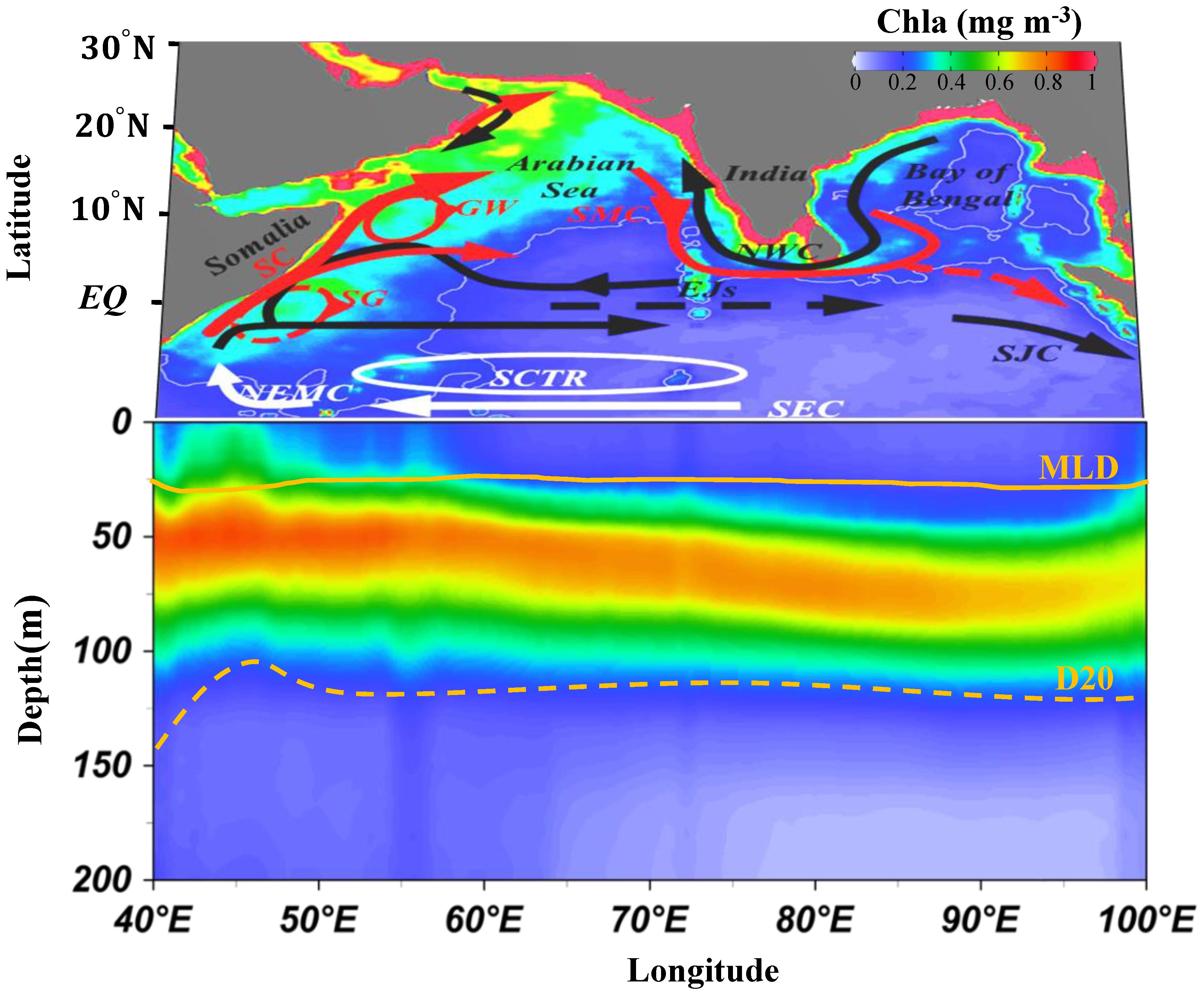
Figure 1. The three-dimensional structure of chlorophyll a in the northern Indian Ocean. The shading represents the spatial distribution of the annual mean Chla (2000–2019). Longitude-depth plot of Chla, D20 and MLD along 10°S–0. The orange dashed and solid curves indicate the D20 and MLD, respectively. The arrowed curve indicates the surface circulation. The red and black curves represent mean flow during summer and winter monsoons, respectively. The white curve represents the mean flow without seasonal reversal. EJs, Equatorial Jets; GW, Great Whirl; SG, Southern Gyre; SC, Somalia Current; SMC, Southwest Monsoon Current; NWC, Northwest Monsoon Current; NEMC, Northeast Madagascar Current; SEC, South Equatorial Current; SJC, South Java Current; SCTR, Seychelles–Chagos Thermocline Ridge; MLD, Mixed Layer Depth.

Phytoplankton variability is closely linked to short–term climate variabilities (Currie et al., 2013; Hays et al., 2005), including the El Niño–Southern Oscillation (ENSO) and Indian Ocean Dipole (IOD). In the NIO, ENSO and IOD represent two dominant climate modes that lead to variability in both physical and biological systems. ENSO is a prominent mode of climate variability in the Earth system. Its occurrence is linked to ocean–atmosphere coupling in the tropical Pacific, with a characteristic frequency of 2–7 years (Currie et al., 2013; McPhaden et al., 2006). During El Niño (La Niña), air-sea interaction contributes to anomalous warming (cooling) of sea surface temperature (SST) and positive (negative) sea level anomalies (SLA) in the central and eastern Pacific Ocean. This is associated with a decrease (increase) in the climatological zonal trade winds, which in turn reduces (enhances) upwelling by deepening (shallowing) the thermocline along the equator via ocean wave dynamics (Amaya, 2019). It is generally observed that ENSO events reach their most pronounced intensity between November and January. The resulting equatorial SST anomalies in the tropical Pacific Ocean trigger large-scale atmospheric teleconnections linked to El Niño, which can contribute significantly to a general warming of the Indian Ocean (Xie et al., 2009).

The IOD is a unique and inherent mode of interannual variability that affects both local and remote regions (Abram et al., 2020; Saji et al., 1999). IOD activity typically develops in early spring, peaks from August to October, and then rapidly decays in November or December (Abram et al., 2020; Currie et al., 2013). The positive IOD event is initiated by the anomalous easterly winds over the equatorial Indian Ocean, resulting in ocean upwelling along the coasts of Java and Sumatra, as well as cold SST anomalies in the eastern Indian Ocean. Like the Bjerknes feedback essential for ENSO events, the wind and SST anomalies reinforce each other in a positive feedback loop. During the positive IOD event, the anomalous easterly winds result in a decrease in the thermocline depth in the eastern Indian Ocean. Then, the characteristic zonal anomaly pattern in sea level height and vertical temperature results from the associated westward Rossby wave, which deepens the thermocline and warms the upper ocean in the western Indian Ocean (Abram et al., 2020; Rao et al., 2010). Moreover, it is also noted that the subsurface temperature anomalies at the thermocline depth tend to start earlier and last longer than the surface IOD signals (Horii et al., 2008). The IOD could be triggered by ENSO or the inherent oscillation mode in the Indian Ocean (Saji et al., 1999; Yue et al., 2021).

In turn, IOD- and ENSO-related oceanic and atmospheric perturbations can also affect the biological processes in the local and distant oceans (Currie et al., 2013; Pandey et al., 2019; Racault et al., 2017). As the base of the aquatic food web, the IOD- and ENSO-induced interannual variability of phytoplankton can affect fisheries and marine ecosystems, which support the livelihoods of many of the riparian countries in the NIO (Beal et al., 2020; Hermes et al., 2019). Chlorophyll a concentration (Chla) is a universal proxy for phytoplankton biomass and is a particularly good indicator of climate change in the marine environment (Hays et al., 2005). Recently, the deployment of ocean color satellites has afforded researchers a continuous and spatially comprehensive view of the recent IOD and ENSO events (Lehahn et al., 2018; Pandey et al., 2019; Racault et al., 2017). Using the 4-year calibrated SeaWiFS data, Yoder and Kennelly (2003) found that the interannual variability of Chla in the tropical oceans is strongly influenced by the ENSO signal. Due to the coastal upwelling induced by anomalous easterly winds, the co-occurrence of El Niño and positive IOD in 1997/1998 was associated with higher surface Chla in the eastern equatorial Indian Ocean (Liu et al., 2021; Susanto and Marra, 2005). Additional effects of the ENSO and IOD events have produced the Chla bloom in the southern Bay of Bengal (BoB) related to the anomalous westward propagating upwelling Rossby waves (Girishkumar, 2022) and the low surface Chla in the Arabian Sea linked to the wind-induced Ekman transport (Huang et al., 2022). Meanwhile, in the southern equatorial Indian Ocean, the 1997/1998 IOD and ENSO episodes drastically decreased the surface Chla due to the propagating downwelling Rossby waves and local wind anomalies (Ma et al., 2014). Using the satellite observational data, Pandey et al. (2019) analyzed the patterns of Chla anomalies in the Indian Ocean induced by IOD and ENSO during the 2006/2007 events. The results showed that sea surface Chla responded asymmetrically to IOD/ENSO over the NIO, with IOD having a stronger influence than ENSO. In addition, the influence of IOD/ENSO on phytoplankton carbon cycling in the Indian Ocean is also investigated. In the western Indian Ocean, the occurrence of El Niño and positive IOD leads to a decrease in primary production (PP), while an increase in PP is observed in the eastern side (Racault et al., 2017). Thus, significant regional variations in phytoplankton are caused by the effects of ENSO and IOD on the oceanic and atmospheric dynamic processes.

The deep Chla maximum (DCM) is generally shown below the mixed layer rather than the surface in the tropical ocean (Figure 1, Cullen, 2015; Cornec et al., 2021; Yasunaka et al., 2021). In the tropical Indian Ocean, within the mixed layer (0-50 m) is highly oligotrophic with very low chlorophyll a concentration in the upper ocean. It is noteworthy, however, that a well-developed DCM exists between the mixed layer bottom and the thermocline at depths of 50-100 m (Figure 1). Unfortunately, the phytoplankton variability below the surface is not captured by satellite-derived Chla, which accounts for about one-fifth of the total biomass in the entire euphotic layer (Hu et al., 2021, 2022; Sammartino et al., 2018). A robust correlation exists between IOD/ENSO events and interannual fluctuations in the subsurface Chla (Hu et al., 2021; Ma et al., 2014; Shi et al., 2023; Yasunaka et al., 2021). In contrast to surface patterns, El Niño causes the subsurface Chla in the equatorial Pacific to be lower in the west and higher in the east (Yasunaka et al., 2021). In the eastern Arabian Sea, the 2015/2016 El Niño warming event enhanced the subsurface phytoplankton owning to a significant increase in light and temperature in the 50–100 m layer (Hu et al., 2021). In addition, a robust subsurface biological response was observed during the decaying period in a positive IOD event due to the shallower thermocline and turbulent mixing in the eastern equatorial Indian Ocean (Li et al., 2022). Thus, phytoplankton varies dynamically in time and space at the ocean’s surface and subsurface. However, these vertical biological processes within the entire euphotic layer over the NIO are less systematically understood due to the limitations of 3-D observational data.

The objective of this study is to examine the IOD- and ENSO-induced vertical variations of phytoplankton within the whole euphotic layer (0–100 m). We use a two–decade (2000–2019) 3-D Chla dataset from our recently developed high-precision remote sensing inversion model (Hu et al., 2023) to distinguish IOD and ENSO contributions to vertical phytoplankton anomalies in the NIO. Although the biological responses are our primary focus, the sea surface winds (SSW), vertical temperature, and thermocline depth are also investigated to explore the physical mechanisms governing changes in vertical phytoplankton. The paper is structured as follows: Section 2 describes the data and methods employed. Section 3 analyses the influence of IOD and ENSO on the vertical structure of biological and physical variables. Finally, Section 4 presents a summary of the main conclusions.

2 Data and methods

2.1 Data

2.1.1 3-D Chla data

The 3-D of Chla over the NIO were generated by the Random Forest (RF) method of Hu et al. (2023). The proposed method employs a data fusion approach to infer the vertical distribution of Chla, integrating satellite and biogeochemical Argo (BGC-Argo) data. As shown in Figure 2, the RF-model infers the 3-D structure of Chla in the NIO using the near-surface information acquired by satellite products and vertical features collected by BGC-Argo floats. The uncertainties derived from BGC-Argo (instrument drift and calibration issues) and satellite products (atmospheric correction) may affect the accuracy of 3-D Chla products. However, it was previously estimated that the vertical Chla profile produced by the RF model was more accurate and robust than the profiles obtained by other methods (i.e., the neural network and numerical modeling) in the NIO (Hu et al., 2023). In this study, the monthly Chla data from 2000 to 2019 with a uniform 0.25° × 0.25°grid for 32 standard depths ranging from 0 to 200 m (0, 1, 2, 3, 4, 5, 7, 8, 10, 12, 14, 17, 19, 23, 27, 31, 36, 41, 47, 54, 61, 69, 78, 87, 97, 108, 120, 133, 147, 163, 181, and 200 m) are selected to reveal the IOD- and ENSO-related vertical phytoplankton anomalies in the NIO (Figure 2).

Figure 2

Figure 2. Diagram illustrating the processing flow for the 3-D structure of Chla inferred from merged satellite and BGC-Argo data using the RF-Model.

2.1.2 Reanalysis data

Monthly SSW data with a 1/4° horizontal resolution was obtained from the Cross–Calibrated Multi-Platform Ocean Surface Wind Velocity Product (CCMP, www.remss.com) for the 2000–2019. The Global Ocean Ensemble Reanalysis of monthly temperature and MLD were obtained on 1/4° horizontal resolution from the CMEMS at https://marine.copernicus.eu/. The vertical profiles of temperature were obtained from 32 vertical levels ranging from 0 to 200 m. The MLD was calculated as the depth at which the potential density is observed to increase in comparison to the density at 10 m depth, corresponding to a temperature decrease of 0.2°C (Hosoda et al., 2010). To indicate the thermocline depth, the 20°C isotherm (D20) depth is calculated by linear interpolation of the vertical temperature profile (Currie et al., 2013).

2.1.3 IOD and ENSO events

In the NIO, IOD and ENSO events are the most significant short–term climate oscillations (Abram et al., 2020; Schott et al., 2009). The interannual signals associated with the IOD and ENSO were characterized using standard indices. The Pacific ENSO signal was represented by the bi-monthly multivariate ENSO index (MEI; Wolter and Timlin, 2011). The empirical orthogonal function (EOF) was employed to calculate the MEI using five variables (specifically, SST, sea level pressure, zonal and meridional components of the surface wind, and outgoing longwave radiation) over the tropical Pacific basin (30°S–30°N and 100°E–70°W), thereby generating a time series of ENSO conditions. The dipole mode index (DMI), which is a measure of the anomalous SST gradient between the western and southeastern equatorial Indian Ocean (50°–70°E, 10°S–10°N, and 90°–110°E, 10°S–0°) during September and November, was used to indicate the intensity of IOD (Saji et al., 1999). In this study, the MEI and DMI from 2000 to 2019 were obtained from the NASA Physical Sciences Laboratory (https://psl.noaa.gov/).

2.2 Methods

2.2.1 Seasonal and trend decomposition

Seasonal and trend decomposition using LOESS (locally estimated scatterplot smoothing, STL) is a very effective and robust method for decomposing time series (Chan and Cryer, 2008; Cleveland et al., 1990; Zhang et al., 2023). STL can decompose a time series into three main components: seasonal term, trend term, and residual term, using an additive model as follows:

$\begin{array}{ll}{Y}_t=Seasona{l}_t+Tren{d}_t+Irregula{r}_t& (1)\end{array}$

Where $Y_t$ represents the time series. The term $Seasona{l}_t$ is a seasonal factor that can be used to capture periodic changes in the time series within a year. $Tren{d}_t$ indicates the long-term trend. $Irregula{r}_t$ is a random factor that can capture changes that cannot be explained by seasonal or long-term trend effects. In this study, the STL function in the R programming language (R Development Core Team, 2011) was used to calculate interannual anomalies for all variables, such as Chla, Temperature, SSW, MLD, and D20. These anomalies represent the residuals ($Irregula{r}_t$) obtained after removing the seasonal cycle ($Seasona{l}_t$) and the long-term trend ($Tren{d}_t$). The occurrence of ENSO and IOD is linked to ocean-atmosphere coupling in the tropical ocean, with a characteristic frequency of 2-7 years. The trend is calculated by fitting a first–degree polynomial over a 7-year Loess window, which removes long–term changes over decades or longer (Currie et al., 2013). Thus, these interannual anomalies ($Irregula{r}_t$) can be attributed to short–term climate oscillations (< 7 years, i.e., IOD and ENSO), and all analyses in this study were performed on these anomalies. A visual example of the removal of the seasonal and trend signals from (in this case) is shown in Figure 3.

Figure 3

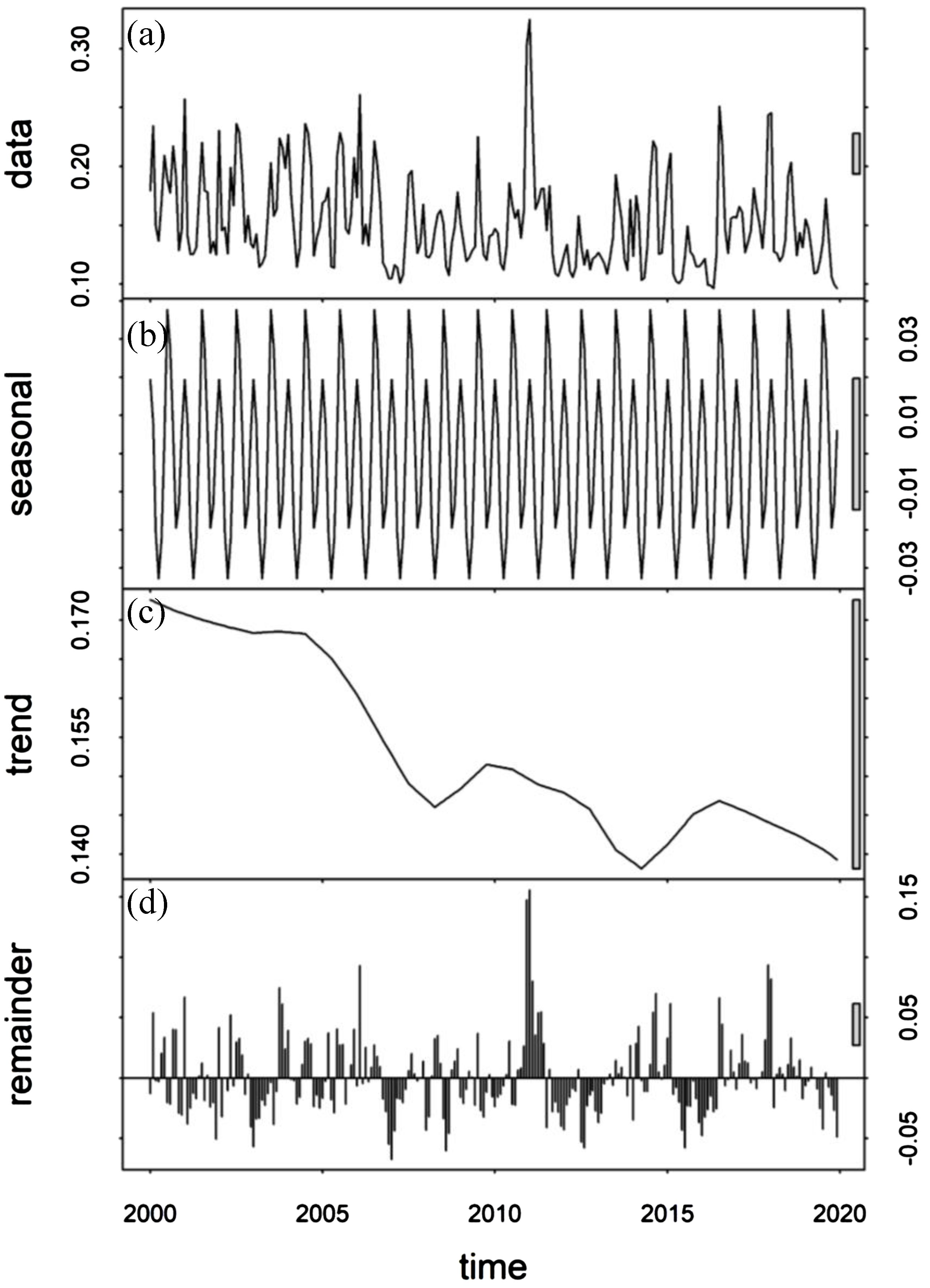
Figure 3. The STL method as applied to Chla. (A) Time-series showing the Chla. (B) Seasonal cycle calculated from $Seasona{l}_t$ of Equation 1. (C) The long-term trend calculated from $Tren{d}_t$ of Equation 1. (D) The residuals obtained after removing the seasonal cycle and the long-term trend from Equation 1.

2.2.2 Partial regression analysis

The primary goal of this paper was to distinguish the effects of IOD and ENSO on biological and physical variables in the NIO. The correlation between IOD and ENSO indices is largely due to the frequent co-occurrence of IOD and ENSO events (Yamagata et al., 2004; Schott et al., 2009). Therefore, partial regression methods were utilized to distinguish the effects of IOD and ENSO, as these techniques have previously been effective in isolating IOD and ENSO signals in physical and biological fields (Saji and Yamagata, 2003; Currie et al., 2013; Keerthi et al., 2013; Pandey et al., 2019). After removing the influence of a third variable from both variables, partial regression is used to determine the effect of one variable on another. For example, to compute the partial regression between a time series of Chla anomalies (CHL) and DMI, while excluding the effect of ENSO, it is necessary to perform three different linear regressions as follows:

$\begin{array}{ll}CHL= a\times MEI+r.CH{L}_{-E}& (2)\end{array}$

$\begin{array}{ll}DMI= b\times MEI+r.DM{I}_{-E}& (3)\end{array}$

$\begin{array}{ll}r.CH{L}_{-E}= c\times r.DM{I}_{-E}+r.CH{L}_{-E-I}& (4)\end{array}$

Moreover, using Equations 5–7, an estimate of the CHL variability linked to ENSO can be calculated excluding the influence of IOD:

$\begin{array}{ll}CHL= a\times DMI+r.CH{L}_{-I}& (5)\end{array}$

$\begin{array}{ll}MEI= b\times DMI+r.ME{I}_{-I}& (6)\end{array}$

$\begin{array}{ll}r.CH{L}_{-I}= c\times r.ME{I}_{-I}+r.CH{L}_{-I-E}& (7)\end{array}$

Where the residuals with ENSO or IOD signals removed are indicated by the subscripts $-E$ and $-I$, respectively. The effect of climate indices on the CHL is estimated by the regression coefficients denoted by the letters a, b, and c. In addition, the climate indices, such as DMI and MEI, have been standardized to a zero mean and unit variance. Consequently, the regression coefficients represent the expected change in the response variable (e.g., CHL), resulting from a climate anomaly with a magnitude of 1. In the above equations, CHL was replaced by SSW, D20, temperature, and MLD anomalies to calculate the effects of IOD and ENSO on these variables, respectively. A visual example of the removal of the linear climate mode (IOD and ENSO) from (in this case) Chla anomalies is shown in Figure 4.

Figure 4

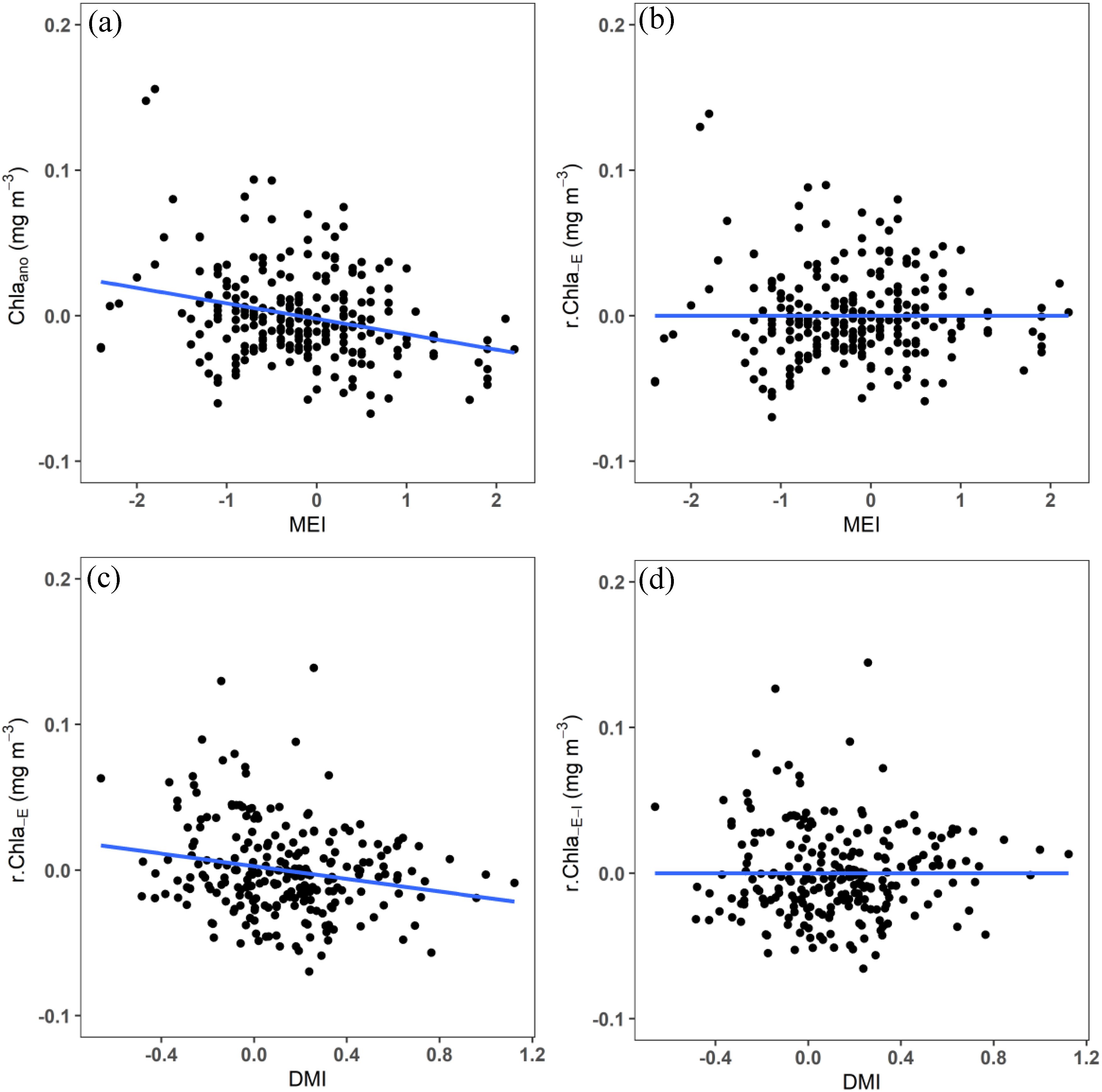
Figure 4. The partial regression method as applied to Chla. (A) Chla anomalies and (B) Chla anomalies residuals from Equation 2, plotted against the MEI index, illustrating the linear relationship with ENSO and its effective removal. The same residuals still have a strong relationship with DMI in (C), but this signal is accounted for by Equation 4, leaving residuals without ENSO or IOD signal (D).

After removing the effect of IOD, the proportion of purely ENSO-induced CHL variance ($V.CH{L}_{MEI}$) was defined as follows (Currie et al., 2013):

$\begin{array}{ll}V.CH{L}_{MEI}=\frac{var(r.CH{L}_{-I})-var(r.CH{L}_{-I-E})}{var(CHL)}& (8)\end{array}$

Where $var(r.CH{L}_{-I})$ and $var(r.CH{L}_{-I-E})$ are the residual variances from Equations 5 and 7, respectively; $var(CHL)$ is the variance of the interannual Chla anomalies. Similarly, the variance associated with the purely IOD-related CHL was calculated as the difference between the residual variances derived from Equations 2 and 4, in relation to the variance of CHL.

3 Results and discussion

3.1 Biological response

Figures 5 and 6 illustrate the regions of pronounced IOD- and ENSO-induced variability of vertical Chla in the upper mixed layer (0–50 m), below the mixed layer (50–100 m), and within the entire euphotic layer (0–100 m), respectively. In the NIO, regions exhibiting pronounced Chla anomalies associated with IOD and ENSO include the Central Arabian Sea (CAS, 60°–70°E, 5°–15°N), the Southern Tip of India (STI, 70°–82°E, 0°–10°N), the Seychelles–Chagos Thermocline Ridge (SCTR, 50°–82°E, 10°–2°S), and the Eastern Equatorial Indian Ocean (EEIO, 90°–100°E, 10°S–0°).

Figure 5

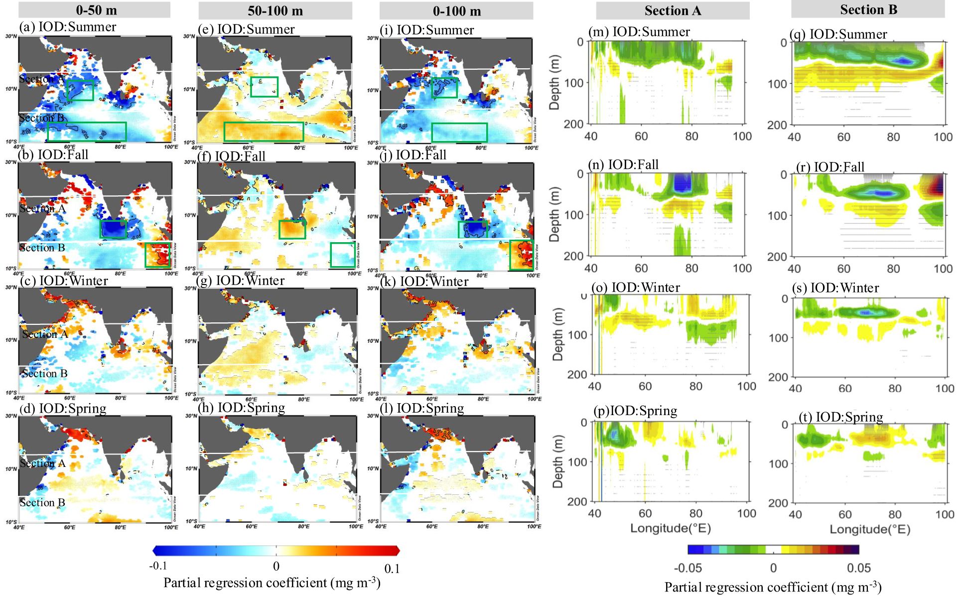
Figure 5. The effect of IOD on the Chla anomalies at (A–D) 0–50 m, (E-H) 50–100 m, and (I-L) 0–100 m in the NIO, as indicated by the partial regression coefficients in Equation 4 (the regression coefficients denoted by the letter c). (M–P) and (Q–T) Same as (A–L), but for vertical structure in section A (40°–100°E, 0-16°N) and section B (40°–100°E, 10°S-0), respectively.The seasonal regressions were performed over the 2000–2019, and only the coefficients exceeding a significance level of 90% were plotted in (A–L). Seasons are represented as June–August (summer), September–November (fall), December–February (winter), and March–May (spring). The geographic boxes represent the selected typical regions.

Figure 6

Figure 6. The influence of ENSO on the Chla anomalies at (A–D) 0–50 m, (E-H) 50–100 m, and (I–L) 0–100 m in the NIO, as indicated by the partial regression coefficients in Equation 7 (the regression coefficients denoted by the letter c). (M–P) and (Q–T) same as (A–L), but for vertical structure in section A (40°–100°E, 0-16°N) and section B (40°–100°E, 10°S-0), respectively. The seasonal regressions were performed for the years 2000–2019, and only the coefficients exceeding a significance level of 90% were plotted in (A–L). The geographic boxes represent the selected typical regions. Season abbreviations as in Figure 5.

The application of partial regression techniques allows for the statistical identification of anomalous signals that are “purely” connected to a single climate mode (e.g., IOD) after the exclusion of the linear signal associated with a different climate mode (e.g., ENSO; Currie et al., 2013; Pandey et al., 2019). Figure 5 shows the effects of pure IOD on the vertical variability of phytoplankton at 0–50 m, 50–100 m, and 0–100 m, respectively. IOD exerts striking control on Chla at different layers, developing in summer and intensifying in fall. In the 0–50 m layer, a significant positive Chla anomaly continuously develops and intensifies from summer to fall in the EEIO (Figures 5A, B), while strong negative Chla anomalies appear in the CAS, SCTR, and STI. Although the effect of IOD on Chla is relatively weak at 50–100 m, it exhibits the opposite tendency from the 0–50 m layer, with significant positive Chla anomalies appearing in the SCTR and STI (Figures 5E, F). In general, the effect of pure IOD on the vertical structure of Chla anomalies is frequently asymmetric within the entire euphotic layer (0–100 m), with fluctuations at 0–50 m being significantly stronger than those at 50–100 m. Additionally, IOD-related Chla anomalies in the 0–100 m layer show similar patterns to those in the 0–50 m layer (Figures 5I, L). However, it is essential to emphasize that the intensity of the Chla anomaly within the entire euphotic layer (0–100 m) is significantly weaker than that in the 0–50 m layer (Figures 5M–T).

As shown in Figure 6, the biological response to ENSO in the NIO is generally weaker compared to IOD. From summer to fall, ENSO–induced negative Chla anomalies at 0–50 m are found in the CAS and STI. During winter and spring, ENSO dominates the vertical variability of Chla anomalies in the CAS and SCTR. The largest ENSO-related Chla anomaly signal appears to be observed in the SCTR. The negative Chla anomalies at 0–50 m layer are gradually weakened in the CAS (Figures 6C, D), accompanied by continuously increasing negative (positive) Chla anomalies in the 0–50 m (50–100 m) layer in the SCTR from winter to spring (Figures 6G, H). Compared with IOD, the occurrence of ENSO-related Chla anomalies is typically delayed by at least one season (Figure 6). Previous studies have revealed that ENSO has a weaker and delayed effect on surface phytoplankton anomalies compared to IOD (Currie et al., 2013; Pandey et al., 2019). This study further confirmed that the lagged effect of ENSO is ubiquitous within the entire euphotic layer (0–100 m) in the NIO (Figure 6). Like IOD, the opposite change of ENSO-induced Chla anomalies at different depths significantly reduces the variation in Chla anomalies within the whole euphotic layer (0–100 m, Figures 6M–T). This also implies that relying solely on changes in surface phytoplankton may not accurately reflect IOD- and ENSO-induced phytoplankton anomalies in the whole euphotic zone.

The vertical distribution of phytoplankton in the NIO is primarily constrained by the availability of nutrients (Currie et al., 2013; Hu et al., 2023; Li et al., 2022; Liao et al., 2020). Thermocline dynamics processes significantly regulate nutrient supply within the upper mixed layer through vertical mixing and transport (Ma et al., 2014; Marshall et al., 2023; Shi et al., 2023; Williams and Follows, 2003). The shallow thermocline induced by upwelling Rossby waves can facilitate the transport of nutrients into the upper ocean. Within the euphotic layer, the nutrients are rapidly utilized by the biota and contribute to the intense biological activities (Cipollini et al., 2001; Ma et al., 2014; Uz et al., 2001). Despite sufficient light support in the tropical Indian Ocean, oligotrophic conditions prevail in the upper mixed layer due to strong stratification, resulting in a lower biomass in the mixed layer (Figure 1; Hu et al., 2022; Keerthi et al., 2013). Here, we found that Chla anomalies at 0–50 m are negatively related to thermocline depth mainly in these typical regions (Figure 7A, i.e., CAS, STI and SCTR). Thus, IOD- and ENSO-linked thermocline depth anomalies in the CAS, STI, and SCTR may displace subsurface nutrient-rich waters from the bottom mixed layer, thereby limiting phytoplankton growth at 0–50 m. Phytoplankton dynamics have traditionally been attributed to the changes in “bottom–up” environmental variables that influence phytoplankton division rates, such as nutrients and light (Behrenfeld and Boss, 2014). In addition, the ecosystem may also influence phytoplankton biomass via top–down grazing and sinking controls (Arteaga et al., 2020). IOD- and ENSO-induced deeper thermocline may exacerbate the oligotrophic environment in the mixed layer (0–50 m), hence reducing the phytoplankton cell density and predator–prey encounter rates within the euphotic layer. At the same time, our results confirm that Chla anomalies at 50–100 m have a significant positive correlation with D20 in the CAS, STI, and SCTR (Figure 7B). Therefore, the low grazer concentrations, and the IOD- and ENSO-induced deeper thermocline may also drive the vertical migration of phytoplankton and nutrients from the upper mixed layer to the deeper layers (Behrenfeld and Boss, 2014; Wirtz et al., 2022), thus increasing phytoplankton biomass at 50–100 m. Overall, the IOD- and ENSO-induced anomalous dynamic (thermocline depth) and thermodynamic (temperature) variability exerts a significant influence on the marine biological processes (Keerthi et al., 2013; Li et al., 2021; Ma et al., 2014; Rao et al., 2002, 2010; Saji et al., 1999; Schott et al., 2009; Yue et al., 2021). The details will be discussed in the next section.

Figure 7

Figure 7. (A) Regression of 0–50 m Chla anomalies with D20 anomalies. (B) Regression of 50–100 m Chla anomalies with D20 anomalies. The coefficients from a simple linear regression during 2000–2019 were plotted when exceeding a significance level of 90%.

3.2 Physical response

The changes in SSW, SST, and D20 triggered by IOD and ENSO events have been extensively documented in scientific literature (Abram et al., 2020; Horii et al., 2008; Saji et al., 1999; Schott et al., 2009; Yue et al., 2021). Here, we mainly focus on the physical processes (i.e., upwelling, the mixed layer depth and the thermocline depth) that are closely related to the vertical distribution of phytoplankton.

Figure 8 shows how IOD affects physical processes in the NIO. The physical variability triggered by IOD events intensifies in summer and peaks in fall, which is characterized by the zonal gradients of D20 in the equatorial region (Figures 8A, B). Changes in D20 are directly driven by local wind anomalies (Figure 8, Li et al., 2022; Rao et al., 2002). During summer and fall, a pronounced easterly anomaly develops over the equator, leading to the generation of upwelling-favorable equatorially trapped Kelvin waves. These waves propagate into the eastern ocean, causing shoaling of the D20 index in the eastern equatorial region (see Figures 8A, B; Rao et al., 2010). The vertical structure of the upwelling shaped by the coastal trapped Kelvin waves is indicated by the lower temperature at 0–175 m in the eastern Indian Ocean (Figures 8E, F, I, J). The cold anomaly center existed at 30–100 m depth in the range of 90°–100°E (Figures 8E, F, I, J). Thus, the strong upwelling associated with the shallower thermocline depth might be related to the significantly positive Chla anomaly signal in the EEIO. However, compared to the southern hemisphere regions (Section B, 40°–100°E, 10°S-0), the IOD-linked upwelling signals in the northern hemisphere (Section A, 40°–100°E, 0-16°N) do not result in corresponding signals in the overlying temperature anomalies (0–30 m) due to the stronger near-surface salinity stratification in the southern part of the BoB (Figures 8E, F; Sarma et al., 2016). Thus, the corresponding biological response is also restricted to the subsurface layer (50–100 m) in the southern BoB (Figures 5A, E).

Figure 8

Figure 8. (A–D) The effect of IOD on SSW (arrows), D20 (shading), and MLD (contours), as indicated by the partial regression of their anomalies regressed on the IOD index (DMI), after excluding the ENSO signal (Equations 2–4). The red and blue contours in (A–D) represent positive and negative MLD anomalies, respectively. (E–H) and (I–L) same as (A–D), but for vertical temperature in section A (40°–100°E, 0-16°N) and section B (40°–100°E, 10°S-0), respectively. Regressions were performed for the years 2000–2019, and only the coefficients in (A–D) exceeding a significance level of 90% were plotted in (A–D). The stippled area in (E–L) indicates the significance at a 90% significance level.

Simultaneously, an upwelling Rossby wave is reflected offshore to the west on either side of the equator. As shown in Figures 8A and B, this phenomenon can be observed as two negative D20 anomaly lobes. Further west along the equator, the physical processes are primarily influenced by off–equatorial convergence, which is driven by Ekman pumping on the flanks of the equatorial easterly anomaly (Figure 8, Currie et al., 2013). As a result, the STI and SCTR regions exhibit a deeper D20, which propagates westward as symmetrical downwelling Rossby wave signals on both side of the equator in fall (Figure 8B). Significant downwelling due to IOD-related deepening of the thermocline depths is also well characterized by subsurface warming in the STI (Section A, 60°–80°E, Figure 8F) and SCTR (Section B, 60°–80°E, Figure 8J) regions. The enhanced downwelling centers are in the SCTR during fall, with subsurface warm anomalies extending to a depth of 200 m (Figures 8I, J). Downwelling affects the nutrient supply in the euphotic zone, which is essential to support the growth of phytoplankton in different layers. Thus, the IOD-related stronger downwelling in the STI and SCTR regions may facilitate the formation of opposing biological signals in the 0–50 m and 50–100 m layers. Further west, in the CAS, an IOD-linked shallower MLD anomaly is identified (Figure 8A), which may account for the significant negative Chla anomaly at the 0–50 m layer (Figure 5A).

Like IOD, ENSO has exerted a strong influence on the tropical Indian Ocean thermocline during the last two decades (2000–2019, Figures 9C, D). When the IOD-related D20 and temperature signals dissipate in winter (Figure 8C), the influence of the ENSO signal strengthens in winter and peaks in the following spring (Figures 9C, D), lasting about one season. Compared to IOD, ENSO-linked equatorial easterly wind anomalies also result in a shallower D20 in the EEIO (Figure 9C, Rao and Behera, 2005). At the same time, the D20 deepens in the SCTR region in response to Ekman pumping (Figures 9C, D; Currie et al., 2013). In the southern hemisphere (Section B), these subsurface anomalies are much larger than those of the IOD (Figures 6K, L). The deeper D20 and amplified MLD interact with the normally shallow SCTR to make the downwelling more noticeable and persistent in the SCTR region (Figures 9K, L, Dilmahamod et al., 2016; Yokoi et al., 2008). Meanwhile, the ENSO-related downwelling warm center is located at a depth of 10–100 m (Figures 9K, L), which is significantly shallower than that of the IOD. The relatively shallower downwelling provides favorable conditions for positive Chla anomalies below the mixed layer (50–100 m, Figure 6H). However, in the EEIO (Section A), the strong upwelling induced by the equatorial easterly anomaly is persistently limited to depths below 50 m. This phenomenon can be attributed to the monsoon–related wind reversal in the southern BoB (see Figures 9C, D, Schott et al., 2009), which inhibits the upwelling of cold, nutrient-rich waters into the upper mixed layer (see Figures 8G, H). Consequently, this limits biological activity within the entire euphotic layer (0–100 m, Figure 6).

Figure 9

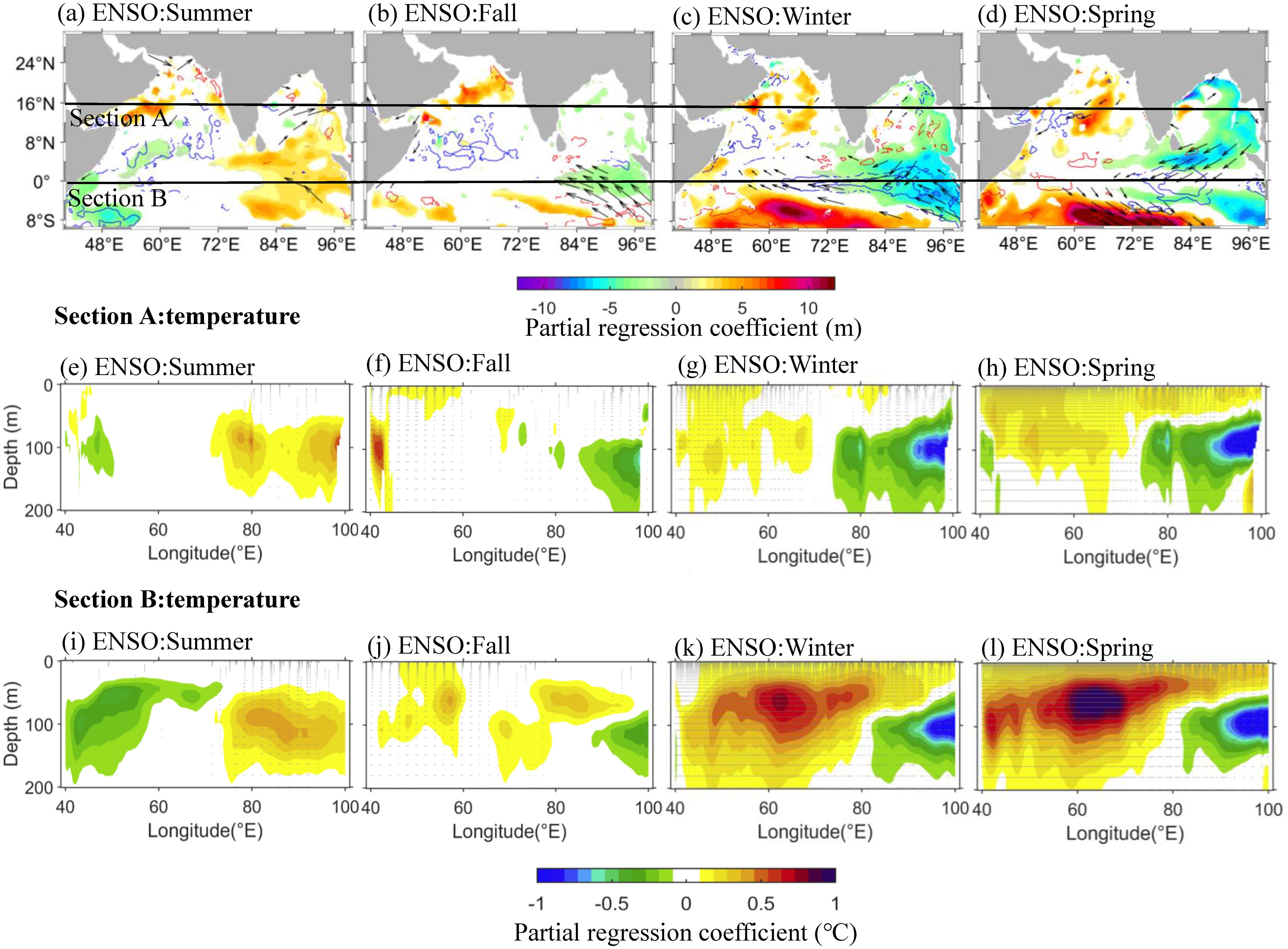
Figure 9. (A–D) The effect of ENSO on SSW (arrows), D20 (shading), and MLD (contours), as indicated by the partial regression of their anomalies regressed on the ENSO index (MEI), after excluding the IOD signal (Equations 5–7). The red and blue contours in (A–D) represent positive and negative MLD anomalies, respectively. (E–H) and (I–L) same as (A–D), but for vertical temperature in section A (40°–100°E, 0–16°N) and section B (40°–100°E, 10°S–0), respectively. Regressions were performed for the years 2000–2019, and only the coefficients in (A–D) exceeding a significance level of 90% were plotted in (A–D). The stippled area in (E–L) indicates the significance at a 90% significance level.

3.3 Vertical structure in key regions

As shown in Figures 5, 6 and 8, 9, the biological and physical responses to ENSO and IOD forcing exhibit spatial and temporal differences. Here, we examine the vertical structure of the Chla anomalies and their seasonality in more detail by focusing on several key regions (i.e., CAS, STI, SCTR, and EEIO; Figure 10), where exhibit the strongest IOD- and ENSO-induced physical and biological signals in the NIO (Figures 5–9).

Figure 10

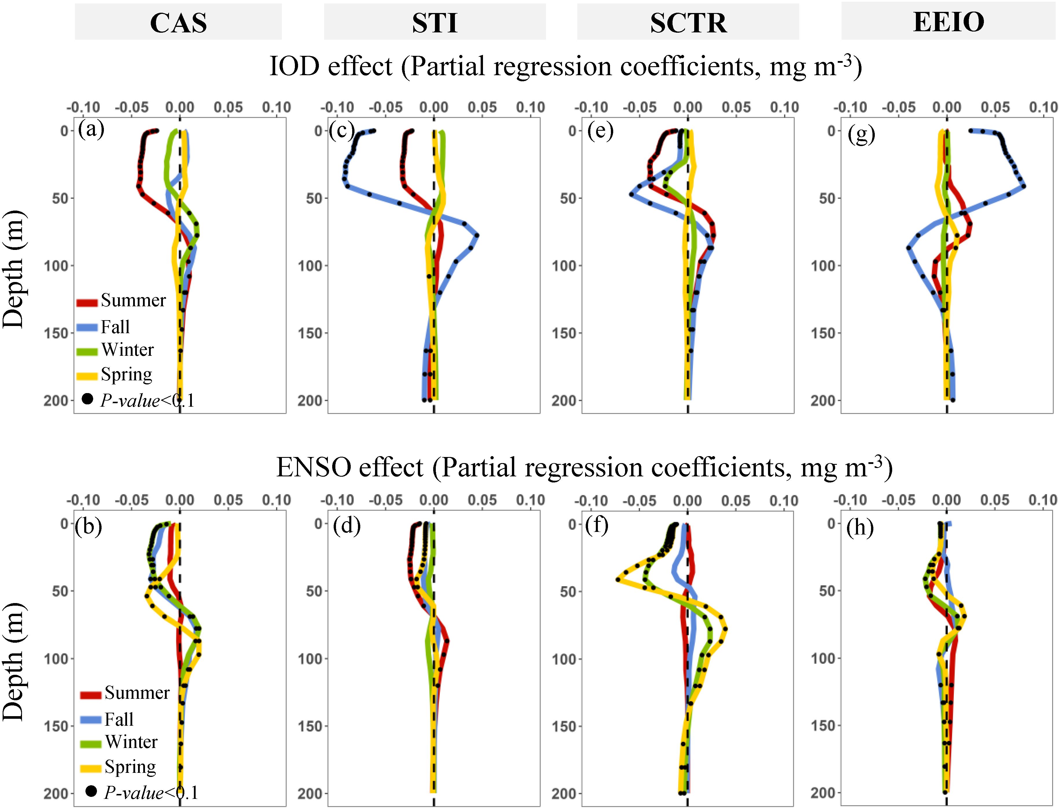
Figure 10. (A–H) Seasonal evolution of the IOD– and ENSO–induced Chla anomalies (CHL) during 2000–2019. ENSO and IOD effects are indicated by partial regression coefficients (Equations 2–4 for pure IOD effect; Equations 5–7 for pure ENSO effect). (A, B) The Central Arabian Sea (CAS). (C, D) The Southern Tip of India (STI). (E, F) The Seychelles–Chagos Thermocline Ridge (SCTR). (G, H) The Eastern Equatorial Indian Ocean (EEIO).

In the CAS region, the largest negative Chla anomalies at the 0–50 m layer in summer respond to pure IODs (Figure 10A), as indicated by a relatively high variance explained rate (~40%, Figure 10A). These negative anomalies follow a MLD shoaling and coincide with warmer-than-normal temperature at the 0–50 m layer (Figure 8E). In winter, the biological activity in the CAS is mainly influenced by ENSO, with a larger proportion of vertical variability of Chla (40~50%, Figure 11C). Similar to IOD, significant negative Chla anomalies in the 0–50 m layer are observed in response to ENSO in winter (Figure 10B). Conversely, ENSO-related weak positive Chla anomalies are found at the 50–100 m layer (Figure 10B). Meanwhile, the ENSO causes a deeper thermocline and MLD shoaling, and soon thereafter, a warm temperature at 0–100 m from winter to spring (Figures 9G, H). The IOD- and ENSO-induced shallower MLD likely contributes to lower nutrient concentrations at the 0–50 m layer (Hu et al., 2021), thereby limiting the phytoplankton growth in the mixed layer (0–50 m). In addition, the deeper thermocline in the CAS can result in downwelling following the spring ENSO event (Figure 9D), which further exacerbates the oligotrophic environment in the upper mixed layer. The downwelling process also transports phytoplankton and nutrients from the mixed layer to the deeper layer (50–100 m).

Figure 11

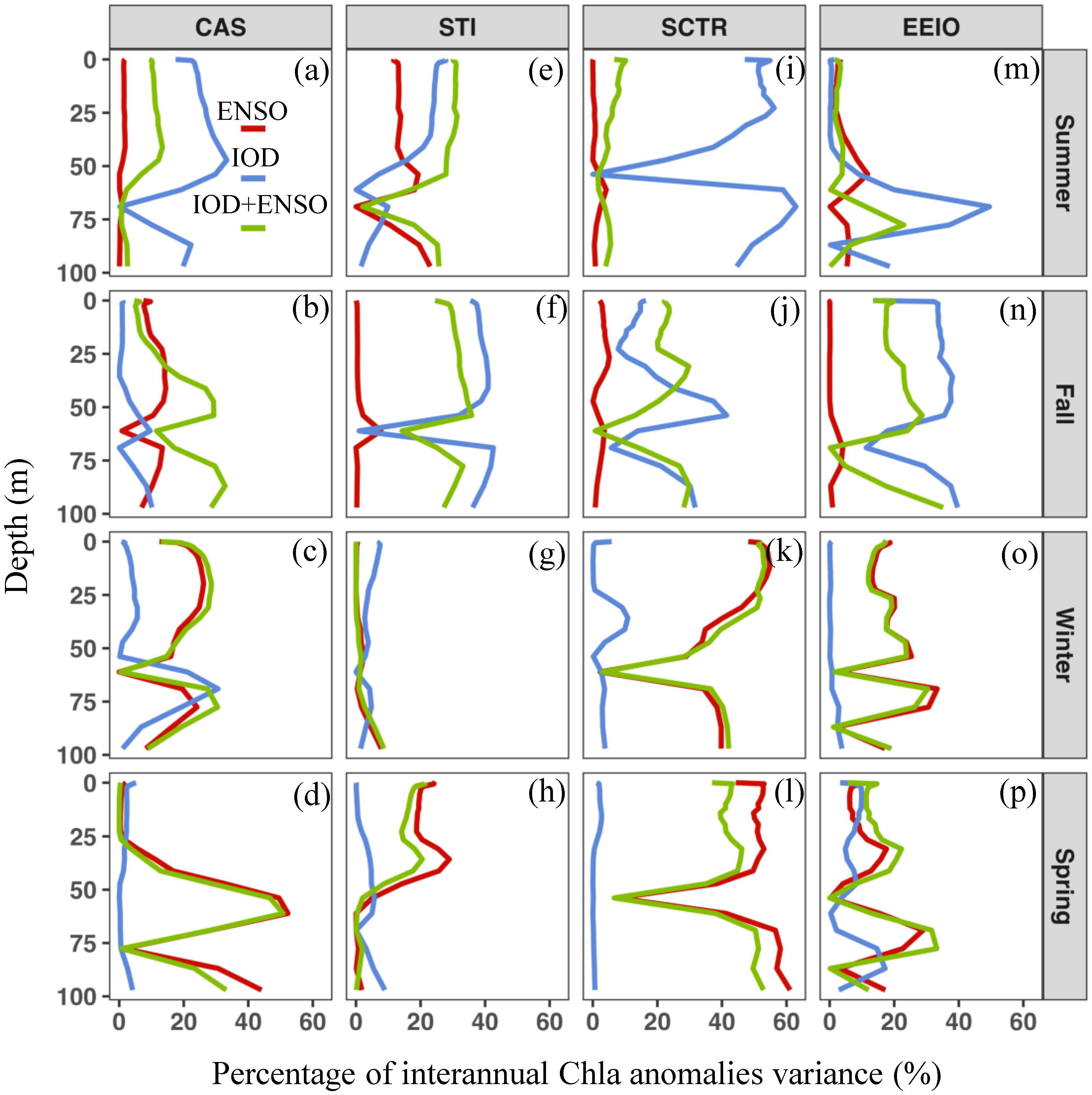
Figure 11. (A–P) Percentage of interannual Chla anomaly variance explained by pure IOD, purely ENSO, and IOD+ENSO, respectively. The IOD+ENSO indicates the DMI+MEI as explanatory variables. (A–D) The Central Arabian Sea (CAS). (E–H) The Southern Tip of India (STI). (I–L) The Seychelles–Chagos Thermocline Ridge (SCTR). (M–P) The Eastern Equatorial Indian Ocean (EEIO).

In the STI region, the largest negative Chla anomaly is closely related to IOD and occurs in summer and fall (Figure 10C). IOD induces a significant opposite change trend at 0–50 m and 50–100 m. The positive IOD can lead to a significant negative (positive) Chla anomaly at 0–50 m (50–100 m) in fall (Figure 10C). In addition, we found that the co-occurrence of ENSO and IOD during summer and fall explains a relatively high proportion of the Chla anomalies (~40%; Figures 11E, F). In the STI, the vertical distribution of Chla is shaped by the open-ocean upwelling, which is primarily driven by the summer monsoon and Rossby wave propagation (Hu et al., 2022; Li et al., 2021; Rao et al., 2010). Here, deeper D20 develops in summer and fall, a result of subsurface warm anomalies triggered by downwelling Rossby waves following a positive IOD and El Niño (Figures 8B, 9A). Thus, the vertical change of Chla anomalies in summer and fall may be reinforced by the co-occurring IOD and ENSO (Figure 9A), due to the similar effects on the thermocline depth in summer and fall (Figures 8B, 9A). The basin–scale response of Indian Ocean phytoplankton to co-occurring events appears to be weak due to opposing regional signals, as observed by Currie et al. (2013). However, in the STI, the co-occurring ENSO and IOD in summer and fall can directly affect the intensity of the open ocean upwelling (Figures 8F, 9E; Li et al., 2021), which would be responsible for the stronger vertical change of the Chla anomalies. During winter and spring, there appears to be a lack of coupling between the 0–50 m temperature and thermocline depth anomalies (Figures 9C, D, G, H) in the STI, likely due to the intense horizontal advection driven by the easterly anomaly (Figures 9C, D), as well as the stratified barrier layer that isolates the surface temperature from the influence of subsurface upwelling (Figures 9G, H; Currie et al., 2013; Schott et al., 2009). Thus, the upwelling cold waters hardly introduce nutrients into the euphotic zone (Figures 9G, H), and ENSO-related Chla anomalies appear to be relatively weak in the STI region (Figures 10D).

In the SCTR region, the percentage of variance of the interannual Chla anomaly explained by the DMI and MEI indices reached 60% (Figures 11I–L). The pure IOD and ENSO significantly affect the vertical structure of Chla anomalies during summer–fall and winter–spring, respectively. IOD and ENSO trigger a negative (positive) Chla anomaly at 0-50 m (50-100 m) (Figures 10E, F). Meanwhile, the variability of D20 is consistent with changes in surface and subsurface temperatures in response to IOD and ENSO (Figures 8A, B, I, J, 9C, D, K, L). In summer and fall, deeper D20 associated with the positive IOD leads to a strong downwelling, as indicated by significant warm anomalies in the subsurface layer (50–100 m; Figures 8A, B, I, J). The stronger downwelling can facilitate the removal of nutrients from the upper mixed layer (McGillicuddy, 2016), thus limiting phytoplankton growth at 0–50 m (Figure 10E). At the same time, the downwelling and oligotrophic environment in the 0–50 m depth layer might push phytoplankton deeper within the euphotic layer (Behrenfeld and Boss, 2014; McGillicuddy, 2016), resulting in an increase in Chla at 50–100 m (Figure 10E). In winter and spring, we found that significant vertical variability in Chla anomalies is associated with pure ENSO (Figure 10F). ENSO-related thermocline anomalies dominate the vertical distribution of Chla from winter until the following spring (Figure 9). Different from a positive IOD event, the subsurface phytoplankton (50–100 m) increases strongly during El Niño, linked to the relatively shallow subsurface warming in winter and spring (Figures 9K, L). This result differs from the findings of Currie et al. (2013) and Rao et al. (2002), which suggest that the interannual vertical variability of phytoplankton in the tropical Indian Ocean is primarily driven by the IOD. However, in the SCTR region, the deeper MLD and shallower thermocline may be intensified during El Niño events in the winter and spring (Figure 9), which may weaken the downward transport of phytoplankton and nutrients from the euphotic zone, thereby sustaining subsurface phytoplankton growth (50–100 m, Figure 9F).

In contrast to the above, a significant positive (negative) Chla anomaly occurs at 0–50 m (50–100 m) occurs in the EEIO following a positive IOD event (Figure 10G). Most previous studies have focused only on surface phytoplankton blooms in the EEIO (Pandey et al., 2019; Susanto and Marra, 2005; Vinayachandran et al., 2021). Here, the coastal upwelling induced by a strong easterly anomaly can result in the entrainment of nutrients into the euphotic zone (Williams and Follows, 2003), hence boosting phytoplankton growth at 0–50 m. At the same time, the upward vertical transport processes induced by coastal upwelling, along with more plentiful light, allowed the subsurface phytoplankton to migrate upward, resulting in a modest decrease in phytoplankton at 50–100 m (Figure 10G). In addition, ENSO seemingly exerts a significant influence on the thermocline during winter and spring (Figures 9C, D). However, the monsoon-induced wind reversal in the northern hemisphere limits the subsurface upwelling to inject deep nutrients into the euphotic layer in the EEIO (Figures 9K, L). Therefore, ENSO have minor influence on the vertical Chla anomalies in winter and spring (Figure 10H).

4 Conclusions

This study demonstrates that IOD and ENSO induce the opposite changes in phytoplankton at depths of 0–50 m and 50–100 m in the NIO. Changes in phytoplankton are often asymmetric across the euphotic layer, with the effects of ENSO and IOD being significantly more pronounced at 0–50 m than at 50–100 m. During summer and fall, in the CAS, STI, and SCTR, IOD-induced wind anomalies lead to the shallower MLD and deeper D20, which can push nutrient–rich waters into the deeper layer and thus limit phytoplankton growth at 0–50 m (Figure 12). At the same time, the increase in phytoplankton occurs in the subsurface layer (50–100 m) because of the downward transport processes of nutrients and phytoplankton. Moreover, due to upwelling caused by a strong easterly anomaly, the IOD-related phytoplankton anomalies in the EEIO exhibit opposite signals compared to other regions over the NIO (Figure 12A). During winter and spring, ENSO has a stronger negative (positive) effect at 0–50 m (50–100 m), due to the local wind anomalies and downwelling Rossby waves. However, in the STI and EEIO, the monsoon-related wind reversal prevents the injection of cold, nutrient-rich water from the deep into the upper layer, thereby limiting vertical biological activity (Figure 12B). The findings may prove valuable in elucidating the response of phytoplankton to variations induced by oceanic dynamics and wind intensity in the context of climate change.

Figure 12

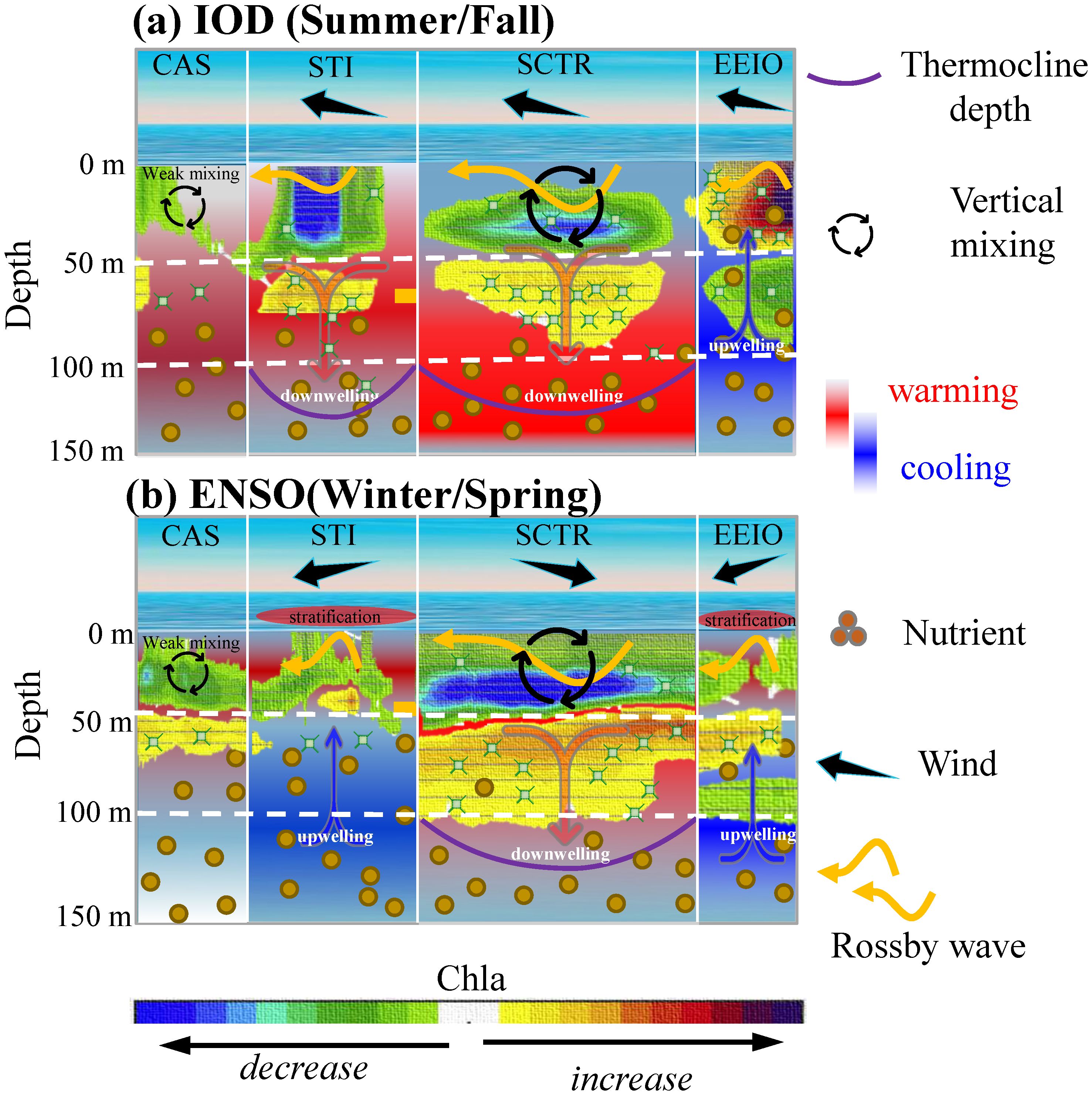
Figure 12. (A, B) Schematic diagram for the vertical variability of phytoplankton within the entire euphotic layer, illustrating the response of phytoplankton to IOD and ENSO events in several key regions in the NIO. (A) IOD effect. (B) ENSO effect.

Moreover, the variance explanation rate also shows that IOD and ENSO have limitations in explaining the vertical variability of interannual phytoplankton (<60%; Figure 11). It is evident that there are regions in the NIO where the vertical variability of phytoplankton is not influenced by either IOD or ENSO. While this study focused solely on two main climate modes (IOD and ENSO), previous studies have illustrated the importance of the intra-annual climate perturbation (e.g., Indian Ocean basin mode, Indian monsoons) and mesoscale phenomena (e.g., eddies, fronts). Complex interactions between the intra-annual climate perturbation and mesoscale phenomena in the Indian Ocean may also influence phytoplankton productivity in the upper ocean (Jiang et al., 2022; Schott et al., 2009; Wang et al., 2021). Future studies will explore how mesoscale features, such as eddies and fronts, interact with IOD and ENSO to influence vertical phytoplankton dynamics in the NIO. Thus, it is therefore important to be cautious when interpreting the vertical structure of phytoplankton anomalies in the context of air-sea interaction processes.

Data availability statement

The datasets presented in this study can be found in online repositories. The names of the repository/repositories and accession number(s) can be found in the article/supplementary material.

Author contributions

QH: Conceptualization, Formal analysis, Funding acquisition, Methodology, Software, Validation, Visualization, Writing – original draft, Writing – review & editing. XC: Formal analysis, Funding acquisition, Supervision, Validation, Writing – review & editing. XH: Conceptualization, Formal analysis, Funding acquisition, Supervision, Validation, Writing – review & editing. YB: Conceptualization, Formal analysis, Funding acquisition, Supervision, Validation, Writing – review & editing. TJ: Conceptualization, Funding acquisition, Supervision, Writing – review & editing. YH: Conceptualization, Formal analysis, Funding acquisition, Writing – review & editing. ZL: Conceptualization, Formal analysis, Validation, Writing – review & editing.

Funding

The author(s) declare financial support was received for the research, authorship, and/or publication of this article. This work was supported by the National Key Research and Development Program of China (Grants #2022YFC3104900 and #2022YFC3104903), the National Natural Science Foundation of China (Grant 42406174 and 62071207), Lianyungang City Science and Technology Project (Grant JCYJ2418), the “Haizhou Bay Talents” Innovation Program of Jiangsu Ocean University (Grant KQ24022), the Natural Science Foundation of Jiangsu Province of China (Grant BK20241064), the Jiangsu Province Marine Science and Technology Innovation Project (Grant JSZRHYKJ202201), the Jiangsu Province Water Conservancy Science and Technology Project (Grant 2020058), and Lianyungang City “521 Project” Scientific Research Project (Grant LYG06521202131).

Conflict of interest

The authors declare that the research was conducted in the absence of any commercial or financial relationships that could be construed as a potential conflict of interest.

Generative AI statement

The author(s) declare that no Generative AI was used in the creation of this manuscript.

Publisher’s note

All claims expressed in this article are solely those of the authors and do not necessarily represent those of their affiliated organizations, or those of the publisher, the editors and the reviewers. Any product that may be evaluated in this article, or claim that may be made by its manufacturer, is not guaranteed or endorsed by the publisher.

References

Abram N. J., Hargreaves J. A., Wright N. M., Thirumalai K., Ummenhofer C. C., England M. H. (2020). Palaeoclimate perspectives on the Indian Ocean dipole. Quat. Sci. Rev. 237, 106302. doi: 10.1016/j.quascirev.2020.106302

Crossref Full Text | Google Scholar

Amaya D. J. (2019). The Pacific meridional mode and ENSO: A review. Curr. Clim. Change Rep. 5, 296–307. doi: 10.1007/s40641-019-00142-x

Crossref Full Text | Google Scholar

Arteaga L. A., Boss E., Behrenfeld M. J., Westberry T. K., Sarmiento J. L. (2020). Seasonal modulation of phytoplankton biomass in the Southern Ocean. Nat. Commun. 11, 5364. doi: 10.1038/s41467-020-19157-2

PubMed Abstract | Crossref Full Text | Google Scholar

Beal L. M., Vialard J., Roxy M. K., Li J., Andres M., Annamalai H., et al. (2020). A road map to IndOOS-2: Better observations of the rapidly warming Indian Ocean. B. Am. Meteorol. Soc 101, E1891–E1913. doi: 10.1175/bams-d-19-0209.1

Crossref Full Text | Google Scholar

Behrenfeld M. J., Boss E. S. (2014). Resurrecting the ecological underpinnings of ocean plankton blooms. Annu. Rev. Mar. Sci. 6, 167–194. doi: 10.1146/annurev-marine-052913-021325

PubMed Abstract | Crossref Full Text | Google Scholar

Chan K. S., Cryer J. D. (2008). Time series analysis with applications in R (New York, NY: Springer Science+Business Media, LLC). doi: 10.1007/978-0-387-75959-3

Crossref Full Text | Google Scholar

Cipollini P., Cromwell D., Challenor P. G., Raffaglio S. (2001). Rossby waves detected in global ocean colour data. Geophys.l Res. Lett. 28, 323–326. doi: 10.1029/1999gl011231

Crossref Full Text | Google Scholar

Cleveland R. B., Cleveland W. S., McRae J. E., Terpenning I. (1990). STL: A seasonal-trend decomposition. J. Off. Stat. 6, 3–73.

Google Scholar

Cornec M., Claustre H., Mignot A., Guidi L., Lacour L., Poteau A., et al. (2021). Deep chlorophyll maxima in the global ocean: Occurrences, drivers and characteristics. Global Biogeochem. Cy. 35, e2020GB006759. doi: 10.1029/2020gb006759

PubMed Abstract | Crossref Full Text | Google Scholar

Cullen J. J. (2015). Subsurface chlorophyll maximum layers: enduring enigma or mystery solved? Annu. Rev. Mar. Sci. 7, 207–239. doi: 10.1146/annurev-marine-010213-135111

PubMed Abstract | Crossref Full Text | Google Scholar

Currie J. C., Lengaigne M., Vialard J., Kaplan D. M., Aumont O., Naqvi S. W. A., et al. (2013). Indian Ocean dipole and El Nino/southern oscillation impacts on regional chlorophyll anomalies in the Indian Ocean. Biogeosciences 10, 6677–6698. doi: 10.5194/bg-10-6677-2013

Crossref Full Text | Google Scholar

Dilmahamod A. F., Hermes J. C., Reason C. J. C. (2016). Chlorophyll-a variability in the Seychelles–Chagos Thermocline Ridge: Analysis of a coupled biophysical model. J. Mar. Syst. 154, 220–232. doi: 10.1016/j.jmarsys.2015.10.011

Crossref Full Text | Google Scholar

Girishkumar M. S. (2022). Surface chlorophyll blooms in the Southern Bay of Bengal during the extreme positive Indian Ocean dipole. Clim. Dyn. 59, 1505–1519. doi: 10.1007/s00382-021-06050-x

Crossref Full Text | Google Scholar

Gruber N., Clement D., Carter B. R., Feely R. A., Van Heuven S., Hoppema M., et al. (2019). The oceanic sink for anthropogenic CO₂ from 1994 to 2007. Science 363, 1193–1199. doi: 10.1126/science.aau5153

PubMed Abstract | Crossref Full Text | Google Scholar

Hays G. C., Richardson A. J., Robinson C. (2005). Climate change and marine plankton. Trends Ecol. Evol. 20, 337–344. doi: 10.1016/j.tree.2005.03.004

PubMed Abstract | Crossref Full Text | Google Scholar

Hermes J. C., Masumoto Y., Beal L. M., Roxy M. K., Vialard J., Andres M., et al. (2019). A sustained ocean observing system in the Indian Ocean for climate related scientific knowledge and societal needs. Front. Mar. Sci. 6. doi: 10.3389/fmars.2019.00355

Crossref Full Text | Google Scholar

Horii T., Hase H., Ueki I., Masumoto Y. (2008). Oceanic precondition and evolution of the 2006 Indian Ocean dipole. Geophys. Res. Lett. 35, L03607. doi: 10.1029/2007gl032464

Crossref Full Text | Google Scholar

Hosoda S., Ohira T., Sato K., Suga T. (2010). Improved description of global mixed-layer depth using Argo profiling floats. J. Oceanogr. 66, 773–787. doi: 10.1007/s10872-010-0063-3

Crossref Full Text | Google Scholar

Hu Q., Chen X., Bai Y., He X., Li T., Pan D. (2023). Reconstruction of 3-D ocean chlorophyll a structure in the northern Indian ocean using satellite and BGC-Argo data. IEEE Trans. Geosci. Remote Sens. 61, 1–13. doi: 10.1109/tgrs.2022.3233385

Crossref Full Text | Google Scholar

Hu Q., Chen X., He X., Bai Y., Gong F., Zhu Q., et al. (2021). Effect of El Niño-related warming on phytoplankton’s vertical distribution in the Arabian Sea. J. Geophys. Res. Oceans 126, e2021JC017882. doi: 10.1029/2021jc017882

Crossref Full Text | Google Scholar

Hu Q., Chen X., He X., Bai Y., Zhong Q., Gong F., et al. (2022). Seasonal variability of phytoplankton biomass revealed by satellite and BGC-argo data in the central tropical Indian ocean. J. Geophys. Res. Oceans 127, e2021JC018227. doi: 10.1029/2021jc018227

Crossref Full Text | Google Scholar

Huang K., Xue H., Chai F., Wang D., Xiu P., Xie Q., et al. (2022). Inter-annual variability of biogeography-based phytoplankton seasonality in the Arabian Sea during 1998–2017. Deep Sea Res.: Top. Stud. Oceanogr. 200, 105096. doi: 10.1016/j.dsr2.2022.105096

Crossref Full Text | Google Scholar

Jiang S., Hashihama F., Masumoto Y., Liu H., Ogawa H., Saito H. (2022). Phytoplankton dynamics as a response to physical events in the oligotrophic Eastern Indian Ocean. Prog. Oceanogr 203, 102784. doi: 10.1016/j.pocean.2022.102784

Crossref Full Text | Google Scholar

Keerthi M. G., Lengaigne M., Vialard J., de Boyer Montégut C., Muraleedharan P. M. (2013). Interannual variability of the Tropical Indian Ocean mixed layer depth. Clim. Dynam. 40, 743–759. doi: 10.1007/s00382-012-1295-2

Crossref Full Text | Google Scholar

Lehahn Y., d’Ovidio F., Koren I. (2018). A satellite-based lagrangian view on phytoplankton dynamics. Ann. Rev. Mar. Sci. 10, 99–119. doi: 10.1146/annurev-marine-121916-063204

PubMed Abstract | Crossref Full Text | Google Scholar

Li H., Zhang J., Wang X., Zhu Y., Liu L., Wang B., et al. (2022). Robust subsurface biological response during the decaying stage of an extreme Indian Ocean Dipole in 2019. Geophys. Res. Lett. 49, e2022GL099721. doi: 10.1029/2022gl099721

Crossref Full Text | Google Scholar

Li Y., Qiu Y., Hu J., Aung C., Lin X., Jing C., et al. (2021). The strong upwelling event off the southern coast of Sri Lanka in 2013 and its relationship with Indian ocean dipole events. J. Clim. 34, 3555–3569. doi: 10.1175/jcli-d-20-0620.1

Crossref Full Text | Google Scholar

Liao X., Du Y., Wang T., He Q., Zhan H., Hu S., et al. (2020). Extreme phytoplankton blooms in the southern tropical Indian Ocean in 2011. J. Geophys. Res. Oceans 125, e2019JC015649. doi: 10.1029/2019jc015649

Crossref Full Text | Google Scholar

Liu H., Sun J., Wang D., Yun M., Narale D. D., Zhang G., et al. (2021). IOD-ENSO interaction with natural coccolithophore assemblages in the tropical eastern Indian Ocean. Prog. Oceanogr. 193, 102545. doi: 10.1016/j.pocean.2021.102545

Crossref Full Text | Google Scholar

Ma J., Du Y., Zhan H., Liu H., Wang J. (2014). Influence of oceanic Rossby waves on phytoplankton production in the southern tropical Indian Ocean. J. Mar. Syst. 134, 12–19. doi: 10.1016/j.jmarsys.2014.02.003

Crossref Full Text | Google Scholar

Marshall T. A., Beal L., Sigman D. M., Fawcett S. E. (2023). Instabilities across the Agulhas Current enhance upward nitrate supply in the southwest subtropical Indian Ocean. AGU Adv. 4, e2023AV000973. doi: 10.1029/2023av000973

Crossref Full Text | Google Scholar

McGillicuddy D. J. Jr. (2016). Mechanisms of physical-biological-biogeochemical interaction at the oceanic mesoscale. Annu. Rev. Mar. Sci. 8, 125–159. doi: 10.1146/annurev-marine-010814-015606

PubMed Abstract | Crossref Full Text | Google Scholar

McPhaden M. J., Zebiak S. E., Glantz M. H. (2006). ENSO as an integrating concept in earth science. Science 314, 1740–1745. doi: 10.1126/science.1132588

PubMed Abstract | Crossref Full Text | Google Scholar

Pandey S., Bhagawati C., Dandapat S., Chakraborty A. (2019). Surface chlorophyll anomalies associated with Indian Ocean Dipole and El Niño Southern Oscillation in North Indian Ocean: a case study of 2006–2007 event. Environ. Monit. Assess. 191, 1–14. doi: 10.1007/s10661-019-7754-z

PubMed Abstract | Crossref Full Text | Google Scholar

Racault M. F., Sathyendranath S., Brewin R. J., Raitsos D. E., Jackson T., Platt T. (2017). Impact of El Niño variability on oceanic phytoplankton. Front. Mar. Sci. 4. doi: 10.3389/fmars.2017.00133

Crossref Full Text | Google Scholar

Rao S. A., Behera S. K. (2005). Subsurface influence on SST in the tropical Indian Ocean: Structure and interannual variability. Dyn. Atmos. Oceans 39, 103–135. doi: 10.1016/j.dynatmoce.2004.10.014

Crossref Full Text | Google Scholar

Rao S. A., Behera S. K., Masumoto Y., Yamagata T. (2002). Interannual subsurface variability in the tropical Indian Ocean with a special emphasis on the Indian Ocean dipole. Deep Sea Res. Part II Top. Stud. Oceanogr. 49, 1549–1572. doi: 10.1016/s0967-0645(01)00158-8

Crossref Full Text | Google Scholar

Rao R. R., Kumar M. G., Ravichandran M., Rao A. R., Gopalakrishna V. V., Thadathil P. (2010). Interannual variability of Kelvin wave propagation in the wave guides of the equatorial Indian Ocean, the coastal Bay of Bengal and the southeastern Arabian Sea during 1993–2006. Deep Sea Res. Part I Oceanogr. Res. Pap. 57, 1–13. doi: 10.1016/j.dsr.2009.10.008

Crossref Full Text | Google Scholar

R Development Core Team (2011). R: A language and environment for statistical computing (Vienna, Austria: R Development Core Team). Available at: http://www.R-project.org (Accessed November 06, 2024).

Google Scholar

Saji N. H., Goswami B. N., Vinayachandran P. N., Yamagata T. (1999). A dipole mode in the tropical Indian Ocean. Nature 401, 360–363. doi: 10.1038/43854

PubMed Abstract | Crossref Full Text | Google Scholar

Saji N. H., Yamagata T. (2003). Possible impacts of Indian Ocean dipole mode events on global climate. Clim. Res. 25, 151–169. doi: 10.3354/cr025151

Crossref Full Text | Google Scholar

Sammartino M., Marullo S., Santoleri R., Scardi M. (2018). Modelling the vertical distribution of phytoplankton biomass in the Mediterranean Sea from satellite data: A neural network approach. Remote Sens. 10, 1666. doi: 10.3390/rs10101666

Crossref Full Text | Google Scholar

Sarma V. V. S. S., Rao G. D., Viswanadham R., Sherin C. K., Salisbury J., Omand M. M., et al. (2016). Effects of freshwater stratification on nutrients, dissolved oxygen, and phytoplankton in the Bay of Bengal. Oceanography 29, 222–231. doi: 10.5670/oceanog.2016.54

Crossref Full Text | Google Scholar

Schott F. A., Xie S. P., McCreary J. P. Jr. (2009). Indian Ocean circulation and climate variability. Rev. Geophys. 47, RG1002. doi: 10.1029/2007rg000245

Crossref Full Text | Google Scholar

Shi Q., Zhang R. H., Tian F. (2023). Impact of the deep chlorophyll maximum in the equatorial pacific as revealed in a coupled ocean GCM-ecosystem model. J. Geophys. Res. Oceans 128, e2022JC018631. doi: 10.1029/2022jc018631

Crossref Full Text | Google Scholar

Susanto R. D., Marra J. (2005). Effect of the 1997/98 El Niño on chlorophyll a variability along the southern coasts of Java and Sumatra. Oceanography 18, 124–127. doi: 10.5670/oceanog.2005.13

Crossref Full Text | Google Scholar

Takahashi T., Sutherland S. C., Sweeney C., Poisson A., Metzl N., Tilbrook B., et al. (2002). Global sea–air CO2 flux based on climatological surface ocean pCO₂, and seasonal biological and temperature effects. Deep Sea Res. Part II Top. Stud. Oceanogr 49, 1601–1622. doi: 10.1016/s0967-0645(02)00003-6

Crossref Full Text | Google Scholar

Uz B. M., Yoder J. A., Osychny V. (2001). Pumping of nutrients to ocean surface waters by the action of propagating planetary waves. Nature 409, 597–600. doi: 10.1038/35054527

PubMed Abstract | Crossref Full Text | Google Scholar

Vinayachandran P. N. M., Masumoto Y., Roberts M. J., Huggett J. A., Halo I., Chatterjee A., et al. (2021). Reviews and syntheses: Physical and biogeochemical processes associated with upwelling in the Indian Ocean. Biogeosciences 18, 5967–6029. doi: 10.5194/bg-18-5967-2021

Crossref Full Text | Google Scholar

Wang Y., Ma W., Zhou F., Chai F. (2021). Frontal variability and its impact on chlorophyll in the Arabian Sea. J. Mar. Syst. 218, 103545. doi: 10.1016/j.jmarsys.2021.103545

Crossref Full Text | Google Scholar

Williams R. G., Follows M. J. (2003). “Physical transport of nutrients and the maintenance of biological production,” in Ocean biogeochemistry: The role of the ocean carbon cycle in global change (Springer Berlin Heidelberg, Berlin, Heidelberg), 19–51. doi: 10.1007/978-3-642-55844-3_3

Crossref Full Text | Google Scholar

Wirtz K., Smith S. L., Mathis M., Taucher J. (2022). Vertically migrating phytoplankton fuel high oceanic primary production. Nat. Clim. Change 12, 750–756. doi: 10.1038/s41558-022-01430-5

Crossref Full Text | Google Scholar

Wolter K., Timlin M. S. (2011). El Niño/Southern Oscillation behaviour since 1871 as diagnosed in an extended multivariate ENSO index (MEI. ext). Int. J. Climato. 31, 1074–1087. doi: 10.1002/joc.2336

Crossref Full Text | Google Scholar

Xie S. P., Hu K., Hafner J., Tokinaga H., Du Y., Huang G., et al. (2009). Indian Ocean capacitor effect on Indo–western Pacific climate during the summer following El Niño. J. Clim. 22, 730–747. doi: 10.1175/2008jcli2544.1

Crossref Full Text | Google Scholar

Yamagata T., Behera S. K., Luo J. J., Masson S., Jury M. R., Rao S. A. (2004). Coupled ocean-atmosphere variability in the tropical Indian Ocean. Earth’s Climate: The Ocean-Atmosphere Interaction. Geophys. Monogr. Ser. 147, 189–212. doi: 10.1029/147gm12

Crossref Full Text | Google Scholar

Yasunaka S., Ono T., Sasaoka K., Sato K. (2021). Global distribution and variability of subsurface chlorophyll a concentration. Ocean Sci. Discuss. 2021, 1–22. doi: 10.5194/os-18-255-2022

Crossref Full Text | Google Scholar

Yoder J. A., Kennelly M. A. (2003). Seasonal and ENSO variability in global ocean phytoplankton chlorophyll derived from 4 years of SeaWiFS measurements. Global Biogeochem. Cy. 17, 1112. doi: 10.1029/2002gb001942

Crossref Full Text | Google Scholar

Yokoi T., Tozuka T., Yamagata T. (2008). Seasonal variation of the Seychelles dome. J. Clim. 21, 3740–3754. doi: 10.1175/2008jcli1957.1

Crossref Full Text | Google Scholar

Yue Z., Zhou W., Li T. (2021). Impact of the Indian Ocean dipole on evolution of the subsequent ENSO: Relative roles of dynamic and thermodynamic processes. J. Clim. 34, 3591–3607. doi: 10.1175/jcli-d-20-0487.1

Crossref Full Text | Google Scholar

Zhang K., Zhao X., Xue J., Mo D., Zhang D., Xiao Z., et al. (2023). The temporal and spatial variation of chlorophyll a concentration in the China Seas and its impact on marine fisheries. Front. Mar. Sci. 10. doi: 10.3389/fmars.2023.1212992

Crossref Full Text | Google Scholar