 Emmaline Sheahan
 Hannah Owens
 Robert Guralnick
 Gavin Naylor1†
94% of researchers rate our articles as excellent or good
Learn more about the work of our research integrity team to safeguard the quality of each article we publish.
Find out more
ORIGINAL RESEARCH article
Front. Mar. Sci., 06 March 2025
Sec. Marine Biology
Volume 12 - 2025 | https://doi.org/10.3389/fmars.2025.1521474
Introduction: Discoveries of coelacanth populations off the East African coast and in the Indo-Pacific warrant an analysis of their potential distributions, but the necessary tools to model and project their distributions in 3 dimensions are lacking.
Methods: Using occurrence records for the West Indian ocean coelacanth, Latimeria chalumnae, we produced 3D and 2D maximum entropy ecological niche models and projected them into the habitat of the Indonesian coelacanth, Latimeria menadoensis. We gauged each model’s success by how well it could predict L. menadoensis presences recorded from submersible observations.
Results: While the 2D model omitted 33% of occurrences at the most forgiving threshold, the 3D model successfully predicted all occurrences, regardless of threshold level.
Discussion: Incorporating depth results in improved model accuracy when predicting coelacanth habitat, and projecting into 3 dimensions can give us insights as to where to target future sampling. This 3D modelling framework can help us better understand how marine species are distributed by depth and allow for more targeted conservation management.
There is likely no more famous example of a Lazarus taxon than the coelacanth (Actinistia). The unique clade has captured the attention of researchers and piqued the public’s interest for nearly ninety years since its rediscovery. Coelacanths are a lineage of Sarcopterygian (lobed-fin) fishes that date back to the early Devonian (Johanson et al., 2006; Clement et al., 2024) and together with dipnoans are considered closely related to the common ancestor of tetrapods. They were often referred to as the “missing link” between the marine environment and the tetrapod land invasion. Initially believed to have gone extinct in the late Cretaceous, an extant specimen, subsequently named Latimeria chalumnae, was discovered off the mouth of the Chalumna river in South Africa in 1938 (Smith, 1939). A second specimen would not be found until 1952 (Smith, 1953), off Anjouan in the Comoros, where it appears much more abundant than it is off the South African coast (Fricke et al., 2011). A second species, Latimeria menadoensis, was discovered in 1997 off Sulawesi in Indonesia- over 8,000 km from L. chalumnae’s presumed range (Pouyaud et al., 1999). There have since been L. chalumnae captures off Tanzania, Kenya, Mozambique, and Madagascar. Population genetic analysis suggests there are two distinct populations off the Comoros, as well as somewhat smaller, genetically differentiated populations off South Africa and Tanzania (Lampert et al., 2012). Kadarusman et al. (2020) have also found molecular evidence for the existence of two distinct L. menadoensis populations off Indonesia. The ever-widening range of L. chalumnae and the discovery of a second species suggests habitat suitable for coelacanths may be more prevalent than previously thought, and that there may yet be undiscovered populations.
Species distribution modelling is used for understanding both extent of ranges and where to sample further for new populations. For coelacanths, past work has used 2D modelling approaches to make predictions of distributions for both species. In particular, Owens et al. (2012) produced global maps of potential coelacanth habitat, relying on the GARP and MaxEnt algorithms to generate models from 8 L. chalumnae records and 2 L. menadoensis records. Coro et al. (2013) later produced models of coelacanth distributions based on 21 records, simulated absences taken from an expert model, and artificial neural networks. Both groups projected their models onto the Indo-Pacific, the native range of L. menadoensis, and predicted similar suitable habitat concentrated between Sumatra, Borneo, and Southeast Asia.
While these initial efforts have informed coelacanth distributions, 3D models of coelacanth distributions have not yet been applied. L. chalumnae off the Comoros is observed to spend much of the day resting in volcanic caves around 200 m from the surface. At night, they regularly dive to 500 m where temperatures are lower and oxygen levels are higher (Fricke and Hissmann, 2000). Estimates based on gill surface-area to body size ratios suggest that L. chalumnae cannot tolerate temperatures above 26°C as there is not enough dissolved oxygen to meet their respiratory demands (Froese and Palomares, 2000). Very few individuals have been recorded in caves where temperatures exceed 25°C (Fricke et al., 2011). Therefore, a model based on surface data, where temperatures regularly exceed the estimated physiological tolerance for coelacanths, is less likely to accurately predict their distribution than one built using environmental data taken from the depths at which individuals have been recorded. A model generated using only information at the bottom would also likely be misleading, as sediment and slope in these environments are not suitable for L. chalumnae’s preferred volcanic caves below 400 m (Fricke et al., 2011). 2D models in marine environments often must either compress or neglect information which might be relevant because everything must be analyzed as a singular layer. A 3D model would allow for one to use the actual environmental values at the depth at which occurrences are recorded, and could be projected back onto multiple layers to create a 3-dimensional picture of suitable habitat.
Despite the clear need for a 3D modelling framework (Melo-Merino et al., 2020), implementations remain uncommon. Bentlage et al. (2013) provided an example approach for creating 3D ENMs (Ecological Niche Models) for helmet jellyfish, Periphylla periphylla, though with limited depth information. Freer et al. (2020) compared 2 and 3 dimensional ENMs of 10 species of lanternfish around Antarctica using MaxEnt, but the analysis was limited to 7 depth slices. Owens and Rahbek (2023) demonstrated the importance of using environmental data associated with the depth at which a species is recorded to predict suitable habitat for luminous hake, Steindachneria argentea. They trained GLM models using variables from the surface only, from the benthos only, and from the full depth column, and found that each resulted in different model outputs with the full depth column providing the best assessment of ecological niche and distribution. In instances where it is important to correctly assess both niche and distributions to address questions about marine systems, and there is evidence that 2D models are insufficient, 3D models could prove useful.
In this paper, we present a pipeline for generating a three-dimensional ENM for L. chalumnae as a test case for future use on other marine species. Here, we define a 2D model as that which takes environmental information from a single XY plane- in our case, this is a layer where variables are averaged across the coelacanth’s depth range. The 2D model is also only projected back on to that singular XY plane. We define a 3D model as that which pulls environmental information at the X, Y, and Z coordinate where an individual was recorded, uses a background drawn across all accessible depth layers, and can be projected back onto each depth layer to create a 3D representation of suitable habitat. We aim to 1. Assess the accuracy of 2D versus 3D models for an empirical example; 2. describe coelacanth suitable habitat in 3 dimensions in the Mozambique channel and the Indo-Pacific; and 3. identify potential areas of interest in which researchers should direct their attention when searching for further coelacanth populations. We use the voluModel R package developed by Owens and Rahbek (2023) and introduce new functions we developed here that allow greater flexibility in modelling choices to create 3 dimensional models with the commonly used MaxEnt algorithm (Phillips et al., 2006). We examine the outputs of a traditional two-dimensional ENM of L. chalumnae using a single layer of averaged environmental variables versus a three-dimensional ENM using environmental values at the depths at which individuals are recorded. We then project both models onto the natural range of the Indonesian coelacanth, L. menadoensis, to test each model type’s efficacy in predicting the presence of the second species.
We used an inventory published in Smithiana in 2011 detailing every known coelacanth occurrence for both species documented by the Coelacanth Conservation Council (CCC) as the basis for our records (Nulens et al., 2011). We also used records from an additional inventory of catches specific to Madagascar from 2021 (Cooke et al., 2021). The CCC assigns each capture event a unique CCC number, and this could be cross referenced with the records available via GBIF and OBIS by date. For records lacking coordinate information in GBIF or OBIS, we used the locality, distance from the shore, and depth details in the inventory entry to georeference coordinates for the occurrence in QGIS. We recorded the georeference error as the radius of the associated locality in meters. Because the inventory only held 3 records for L. menadoensis, we supplemented this data using a paper published on ROV field surveys of the species performed by Iwata et al. (2019). We georeferenced coordinates for the sites listed in the paper using QGIS. Ultimately, we assembled longitude, latitude, and depth coordinates for 107 L. chalumnae records and 33 L. menadoensis records. Due to L. chalumnae’s critically endangered status, raw occurrence coordinates will not be made public. Data can be made available upon request in the interest of reproducibility. The identifiers and localities of records used in modelling and validation can be found in the supplement (Supplementary Tables 3, 4).
We assembled data for temperature (Locarnini et al., 2019a), salinity (Zweng et al., 2019), apparent oxygen utilization, dissolved oxygen, percent oxygen saturation (Garcia et al., 2019a), density (Locarnini et al., 2019b), conductivity (Reagan et al., 2019), silicate, phosphate, and nitrate concentrations (Garcia et al., 2019b) for the summer and winter seasons at the 1 degree resolution from the NOAA 2018 World Ocean Atlas (Boyer et al., 2019). Unlike some surface-only datasets, WOA data are organized into depth slices. Preliminary Maxent models with a single linear feature class using all of the available variables averaged across depths revealed that nutrients (silicate, phosphate, and nitrate) and oxygen (oxygen utilization, dissolved oxygen, percent oxygen saturation) contributed little to model predictions. We subsequently excluded these from the analysis in order to use the summer and winter temperature, salinity, density, and conductivity variables at the finer ¼ degree resolution. NOAA WOA depth slices are not equal-depth but become coarser with depth; slices are recorded in 5 meter increments from 0 to 100 meters, by 25 meter increments from 100 meters to 500 meters, and by 50 meter increments from 500 meters to 1000 meters. We capped our maximum depth at 800 m, as we believed this would provide an adequate buffer from the deepest occurrence record (611 m) (Supplementary Table 3), resulting in a total of 43 depth slices.
Because L. chalumnae is known to prefer rocky habitats and use volcanic caves and crevices for shelter (Fricke et al., 1991) we also included slope data for the region of interest. We calculated slope in each pixel at each WOA depth slice from the 1 arc minute ETOPO1 bedrock bathymetry layer (Amante and Eakins, 2009) using terra::terrain() (Hijmans, 2024). Finally, we pulled data for northerly and easterly current velocities for June and December given by the Global Ocean Physics Analysis and Forecast provided by the E.U. Copernicus Marine Service (https://doi.org/10.48670/moi-00016). L. chalumnae is considered a slow swimming drift hunter, and so would be influenced by currents when foraging (Hissmann et al., 2000). These data were organized as above into the same depth slices. For the 2D models, pixel values for each variable were averaged across depth slices from the surface to 800 m to produce a singular mean layer.
Given that most of these records were manually curated, many traditional cleaning steps were not required. To prepare the records for 3D modelling, we ensured each occurrence had a unique longitude, latitude, and depth coordinate, and removed coordinates with a georeference error greater than 20 km. Downsampling is a necessary step in ENM in order to account for potential sampling bias. The depth values were indexed to the closest associated depth slice in the environmental data above, and we used a raster from the environmental data set with the desired resolution (¼ degree) and voluModel::downsample() (Owens and Rahbek, 2023) in order to thin the records per depth slice, ensuring that there would only be one record per voxel. The process was similar for the 2D data set, based on longitude and latitude information without depth data. Similarly, we removed duplicates, excluded points with a georeference error greater than 20 km, and downsampled the records using spThin::thin() (Aiello-Lammens et al., 2015). After cleaning and thinning, 58 occurrence records were available for 3D modelling, and 41 records were available for 2D modelling for L. chalumnae. For L. menadoensis, 17 records were available for 3D validation, and 9 records were available for 2D validation. As expected, more points are lost in 2D modelling than 3D, as points with the same latitude and longitude but different depths are counted as different occurrences, while in a 2D setting those points are counted as duplicates. A plot of the cleaned records with their associated depth values for L. chalumnae (Figure 1A) and L. menadoensis (Figure 1B) are shown in Figure 1.
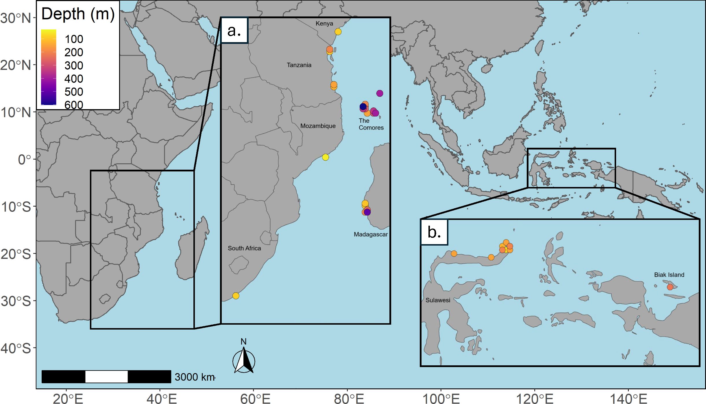
Figure 1. Occurrence records colored by depth of capture for (A) L. chalumnae and (B) L. menadoensis..
For the 3D analysis, we needed to find an appropriate distance with which to buffer the area covered by the points on each depth slice to delimit the accessible area. we used depth slices at 150 and 200m. These were the only depth slices with 7 or more occurrence records. We created 4 different training regions by generating an alpha hull polygon around the occurrence points (voluModel::marineBackground(); Owens and Rahbek, 2023) and buffering it by 4, 6, 8, and 10 times the area covered by occurrence points (proportional size in equation below). We buffered the area covering the points by a distance given by this equation:
We then ran a simple maxent model (1 linear feature class and 1 regularization multiplier) for each slice and each polygon size and pulled the polygon size which produced the model with the lowest AICc: 4 times the area of the points. We then applied this size and used voluModel::marineBackground() to produce an accessible area polygon for each of the 43 depth slices. For each depth slice, we used the occurrences on the slice, as well as those on the slices directly above and below it, as the basis for calculating the buffer in order to create vertical connectivity. We used the same process in order to delineate the accessible area for the 2D model, only using all of the points in order to create a single, all-encompassing 2-dimensional polygon.
We first interpolated the environmental rasters on a by depth layer basis to increase data coverage where reporting was sparse, such as at deeper depths. We did this at each depth slice for every variable except for the slope, since lack of data coverage was not an issue. We accomplished this using voluModel::interpolateRaster(). We then cropped the environmental spatRaster stacks to the accessible area corresponding to their depth slice. We generated a list of 1,000 background points at each depth slice for 43,000 background points in total. We extracted the environmental variable values at the presence and background coordinates to run preliminary maxent models for variable selection. Starting with all of the environmental variables under consideration (summer and winter temperature, density, salinity, and conductivity, northerly and easterly current velocity in December and June, and slope) we ran a simple maxent model (one linear feature class with a regularization multiplier of one) and removed the variable with the lowest permutation importance. We repeated this process until either the Variance Inflation Factor (VIF), a measure of multicollinearity, was less than 10, or until there were only 4 remaining environmental variables. This selection process was adapted from a method used by Abbott et al. (2022). Limiting the number of variables and removing redundant variables reduces overfitting and increases statistical power when presence data are sparse (Sillero and Barbosa, 2021). Ultimately, the slope, Northerly current velocity in December, winter conductivity, and summer temperature were selected as the final suite of variables. We wrote a function in R, maxent_3D(), which could run maxent models of varying parameter sets using a dataframe of environmental variable values extracted at the presence and background coordinates across all depth slices. We tested 4 different feature classes (L, Q, LQ, and LQH) with 4 regularization multipliers for a total of 16 models, the results of which are presented in the supplement (Supplementary Table 1). We used a kfold partition scheme with 5 folds for model validation. We selected the model with the lowest AICc for thresholding, and examined the specificity (the proportion of background correctly predicted as absent) and True Skill Statistic (TSS) at sensitivity values (the proportion of presences correctly predicted as present) of 0.99, 0.95, 0.9, 0.85, 0.8, and 0.75 (Table 1). We used the equation for TSS originally given by Allouche et al. (2006) but down-weighted sensitivity by ⅔ for a final equation of:
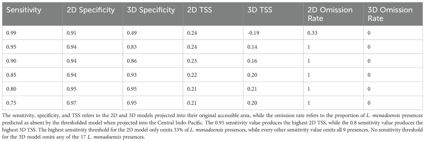
Table 1. The results of thresholding and independent validation using observed L. menadoensis occurrences.
This was done because the ratio of background to presence is generally larger in 3D analyses than for ENMs produced in 2D. Downweighting sensitivity is a means to tune the model in order to reduce model over-commission, thus predicting more of the background as absence. This tuning produced more realistic results than using equal sensitivity and specificity. Additionally, Wunderlich et al. (2019) found that under a variety of modeling scenarios, TSS loses its discriminatory ability as the total number of cells in the analysis increases and species prevalence (ratio of cells where species truly exists to total number of cells) decreases. Increasing the background increases the propensity of false presence and true absence, which can make the specificity - 1 term approach zero, consequently overvaluing the sensitivity term. Given that adding the vertical axis to the analysis greatly increased the background and therefore the total number of cells, we considered downweighting sensitivity a reasonable approach.
The 2D models were produced in a similar fashion as that outlined above. We generated a background of 10,000 points inside of the delineated accessible area, then ran a simple maxent model with a linear feature class and one regularization multiplier using the full list of environmental variables via ENMeval::ENMevaluate() (Kass et al., 2021). We repeated this process, each time removing the variable with the lowest permutation importance, until the VIF was less than 10. Ultimately, summer density, summer conductivity, winter conductivity, the Easterly current in June, the Northerly current in June, the Easterly current in December, the Northerly current in December, and the slope were selected as the environmental variables for the final 2D models. We tested 3 different feature classes (L, LQ, and LQH) with 3 regularization multipliers for a total of 9 models, the results of which can be seen in the supplement (Supplementary Table 2). We selected the model with the lowest AICc for thresholding, this time using the traditional formulation of the TSS given by Allouche et al. (2006):
We thresholded at the same sensitivity values as the 3D analysis, the results of which can be seen in Table 1.
In order to assess the effectiveness of each model to predict the presence of the second coelacanth species, L. menadoensis, we cropped the associated environmental variables at each depth slice to a region over the central Indo-Pacific, extending from 90 to 150 degrees East and 30 degrees South to 30 degrees North. We then projected the best model for L. chalumnae onto this region and thresholded at the 0.99, 0.95, 0.9, 0.85, 0.8, and 0.75 sensitivity values. We recorded the omission rate of the empirically observed L. menadoensis at each sensitivity value. This process was the same for the 2D model, except that the environmental variables in the projected extent were averaged from the surface down to 800 m. The results can be seen in Table 1. We also conducted a MESS (Multivariate Environmental Similarity Surface) analysis in 2D and 3D, and we constructed 3D models using L. menadoensis occurrence records in order to project back into the Mozambique channel, where L. chalumnae is found. The goals of MESS analyses and reciprocal projections were to both understand how different environments were between model training and model projection and to further test model projection results. The outcomes of both of these analyses can be found in the supplement. These analyses were performed in R version 4.3. The code repository for this project can be found at https://github.com/EmmalineSheahan/Coelacanth_3D.
For the 3D analysis, the linear, quadratic, and hinge (LQH) feature class combination with a regularization multiplier of 2 had the lowest average AICc (-5681.20) across the 5 training and testing folds, and was subsequently the model selected for thresholding and projecting (Supplementary Table 1). Every parameter combination produced a relatively high training and validation AUC, with the lowest values- a training AUC of 0.80 and a validation AUC of 0.76- belonging to the model with a quadratic feature class and a regularization multiplier of 4. For the 2D analysis, the linear, quadratic, and hinge (LQH) feature class combination with a regularization multiplier of 3 had the lowest AICc (394.23) across the 5 validation folds, and this was the model selected for thresholding and projecting (Supplementary Table 2). The training and validation AUC values varied minimally across parameter combinations, with the lowest values- a training AUC of 0.88 and a validation AUC of 0.87- belonging to the model with a linear feature class and regularization multiplier of 1.
The 0.80 sensitivity value produced the highest TSS (0.21) for the 3D analysis and was thus selected for thresholding (Table 1). We used the 0.95 sensitivity value to threshold the 2D model, as this produced the highest TSS (0.24). While specificity increased with decreasing sensitivity for both the 3D and 2D analyses, this trend was much more pronounced for the 3D analysis, where specificity was 0.48 at the 0.99 sensitivity value and increased to 0.95 at the 0.75 sensitivity value, as compared to the 2D analysis, where the specificity ranged from 0.91 to 0.96. This may be an artifact of the far higher proportion of background to presence in the 3D model versus the 2D model.
The 2D model predicts generally high suitability around the coastlines of Madagascar and the African continent from Northern South Africa to Southern Somalia, as well as around the Comoros, Seychelles, and other surrounding islands (Figure 2). The 3D model displays much more restricted suitable habitat in the XY plane, with much of it concentrated around Madagascar, the Comoros, Mozambique, Tanzania, and southern Kenya (Figure 3). This suitability increases in scale and scope at depths ranging from 100 to 300 meters, and the thresholded plot displays a great deal of connectivity between depth slices (Figure 4B). The 3D model predicts a much lower proportion of suitable habitat in shallower surface waters, an expected result given known coelacanth depth preferences. Thresholded plots of the 3D model on a per depth slice basis can be found on Figshare (10.6084/m9.figshare.28232696).
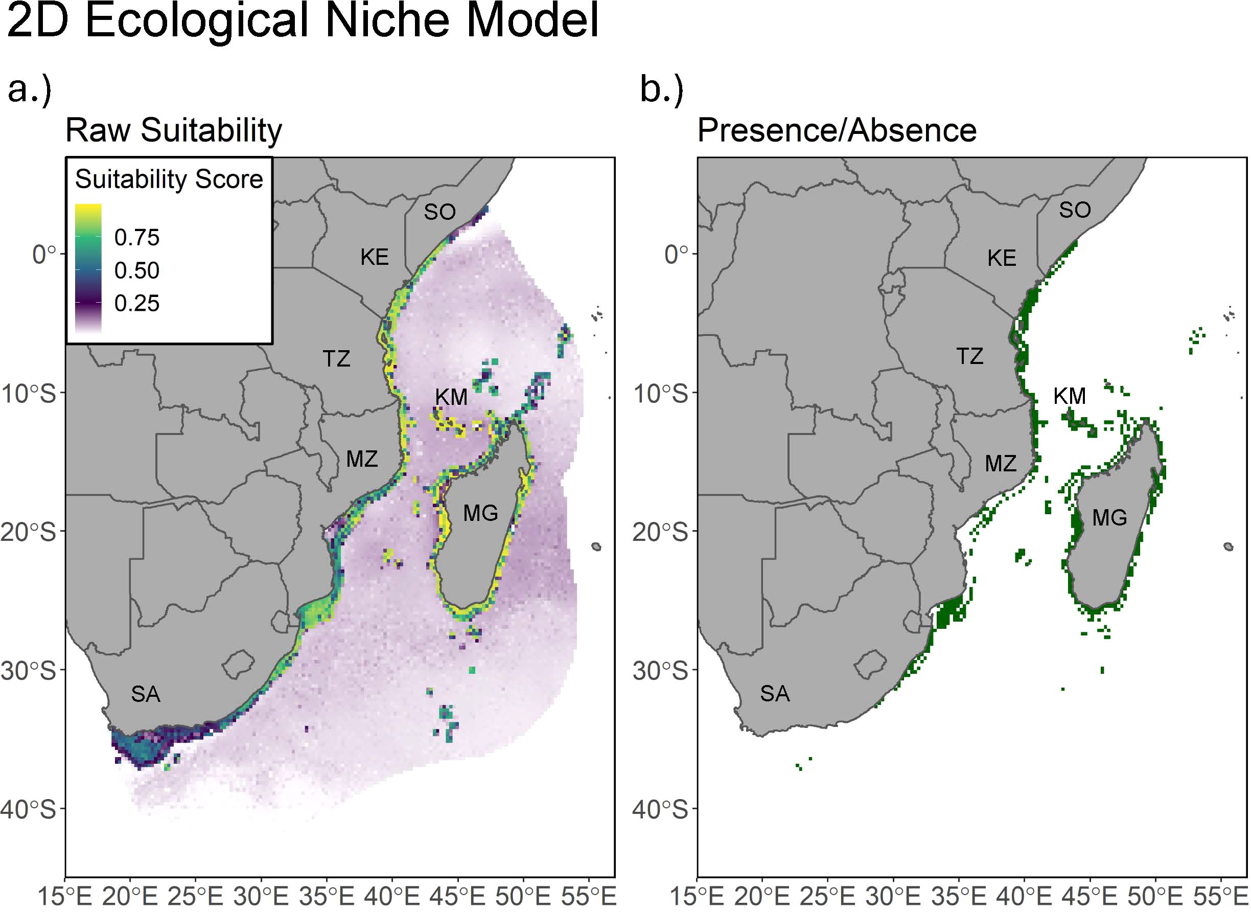
Figure 2. (A) map of suitable habitat for L. chalumnae predicted by the 2D model. A value of 1 indicates high suitability, while a value of 0 indicates low suitability. (B) The thresholded presence of L. chalumnae predicted by the 2D model at the 0.95 sensitivity value. Labels include abbreviated country names.
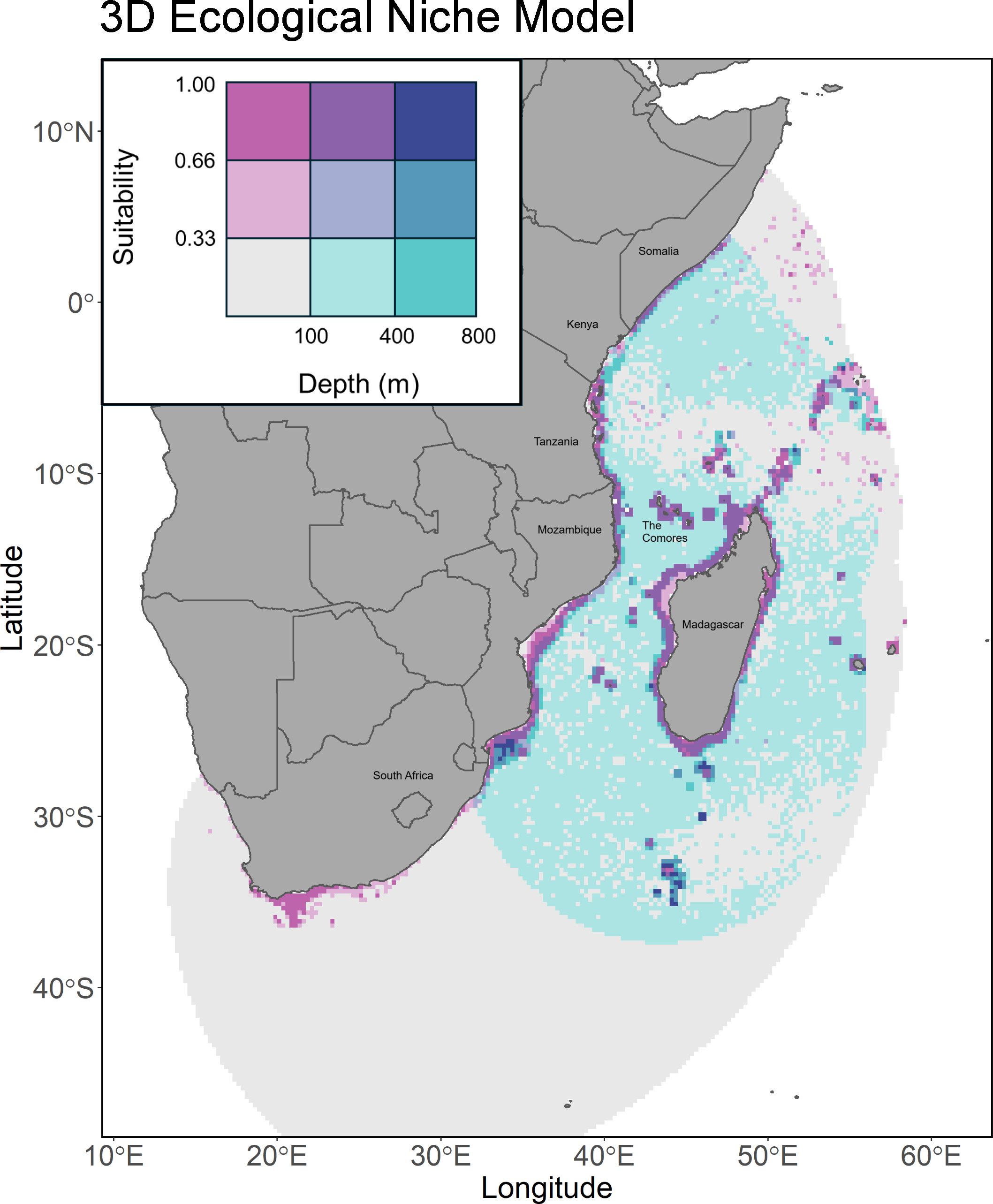
Figure 3. A bivariate chloropleth plot of L. chalumnae suitable habitat predicted by the 3D model. Blue indicates depth, while pink indicates suitability. The darker the blue, the deeper the depth, and the darker the pink, the greater the suitability.
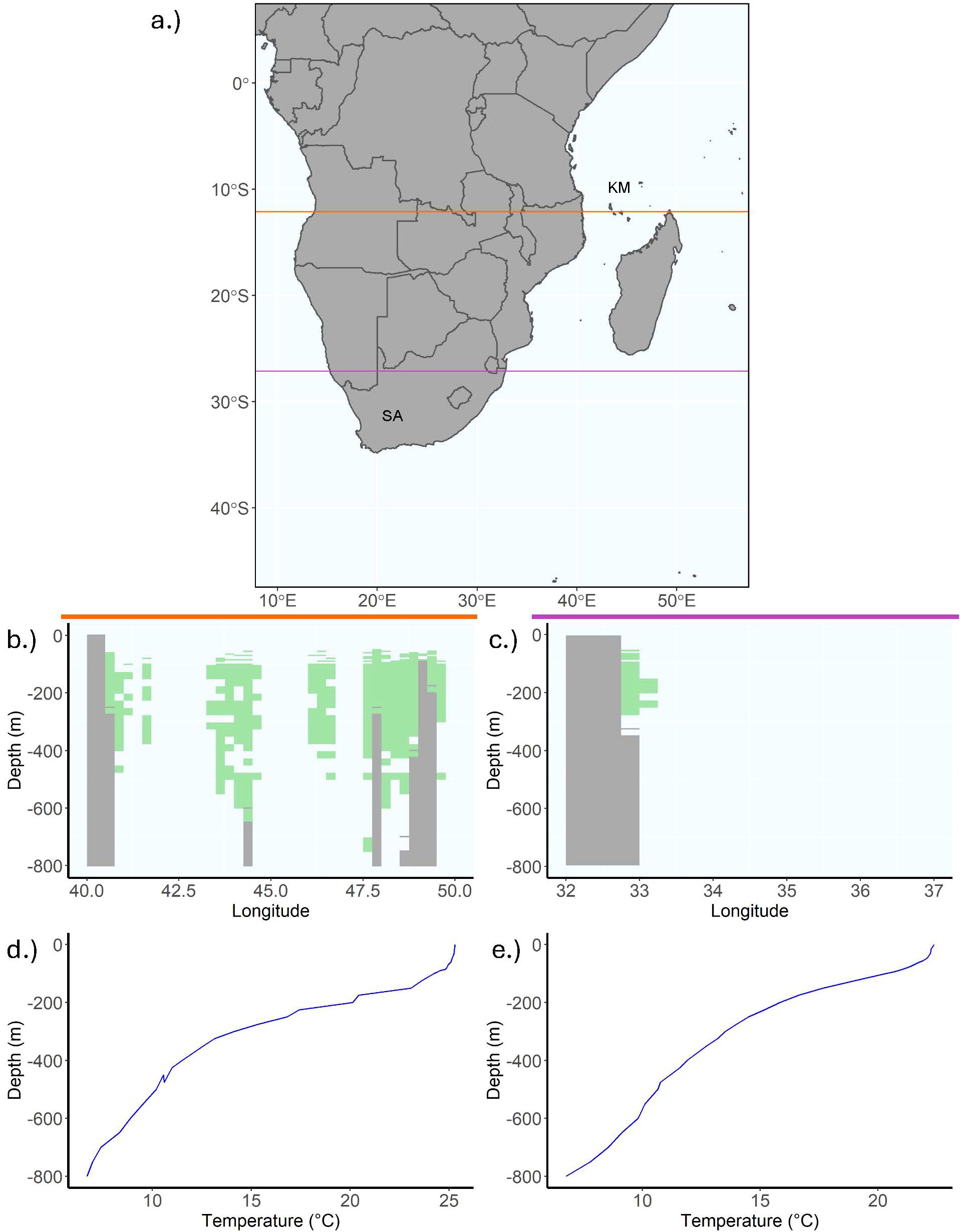
Figure 4. Plots of suitable L. chalumnae habitat by depth thresholded at the 0.8 sensitivity value, with abbreviated country names for South Africa and the Comoros. (A) is a 2D map of the area of interest from South Africa to Somalia, where the orange line at latitude -12.125 intersects the Comoros and corresponds to the two plots in the column below the orange line, and the purple line at latitude -27.125 intersects the Kwa-Zulu Natal and corresponds to the two plots in the column below the purple line. The first two plots below the colored lines depict thresholded coelacanth suitable habitat by depth in green while grey corresponds to either land or the benthos, in (B) the Comoros and off of (C) the Kwa-Zulu Natal. The final two plots depict temperature by depth at a given longitude in (D) the Comoros and off of (E) the Kwa-Zulu Natal. The temperature is about 5 degrees lower and the thermocline begins roughly 50 m shallower off the Kwa-Zulu natal compared to the Comoros.
When projected onto the central Indo-Pacific, the 2D L. chalumnae model predicts a great deal of largely disjointed swaths of suitable habitat, namely between Vietnam and Brunei, along the Northwestern coast of Australia, the Eastern coast of the Philippines, the Western coast of Sumatra, and Western Papua (Figure 5). With the exception of Western Papua, none of the areas are particularly close to Sulawesi or Biak, where L. menadoensis is known to occur, and may reflect commission error. The model does not predict suitable habitat around Sulawesi, the location of the initial discovery of L. menadoensis and many of its subsequent sightings (Erdmann, 1998).
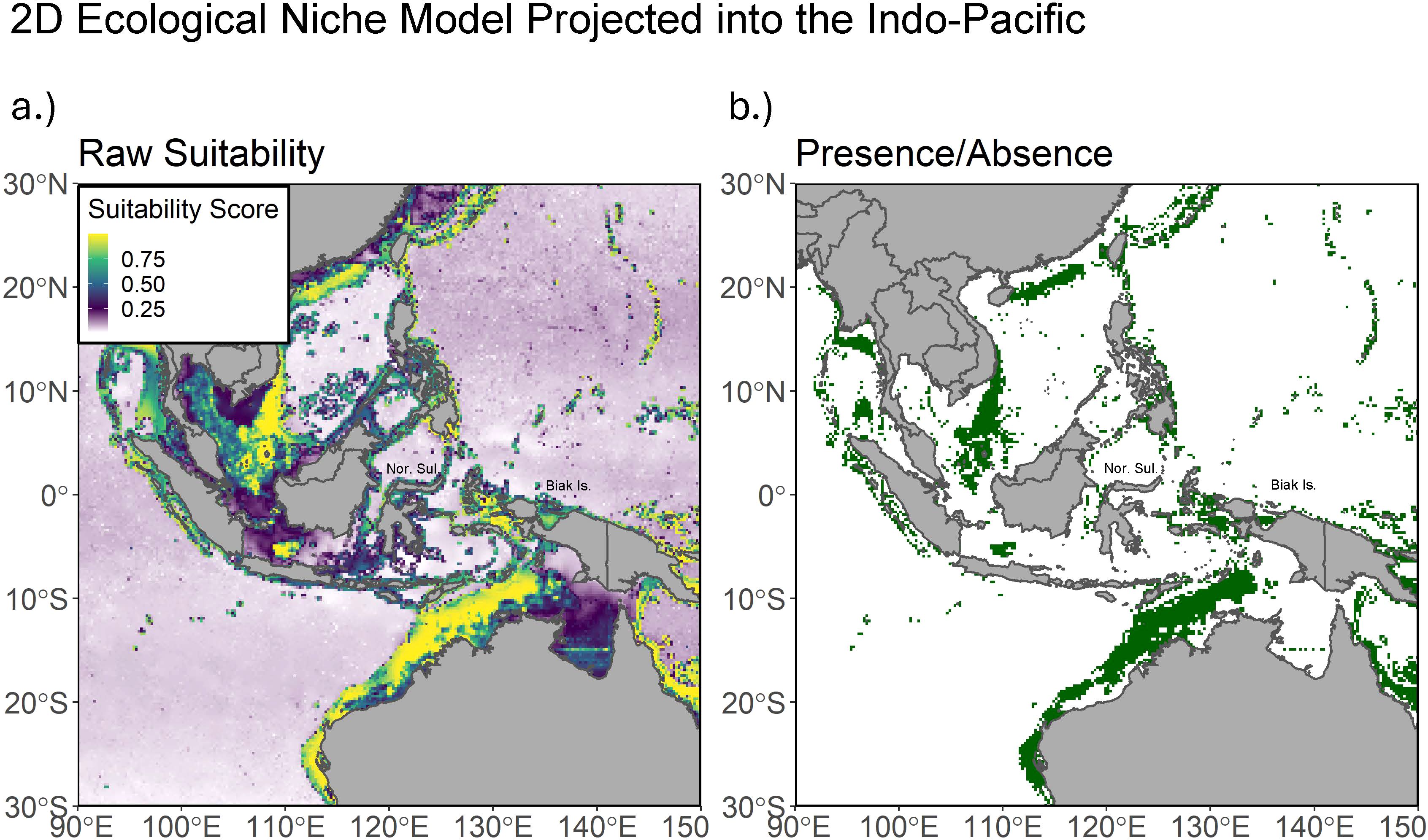
Figure 5. (A) Predicted habitat suitability of the 2D L. chalumnae model projected into the Indo-Pacific, where the sister taxon L. menadoensis resides. (B) The 2D L. chalumnae model projected into the Indo-Pacific and thresholded at the 0.95 sensitivity value. Labels include abbreviations for Northern Sulawesi and Biak Island.
While the projected 3D model appears to predict suitable habitat in the surface waters of Southern China and Taiwan, this is likely due to the influence of cooler temperatures. It also predicts suitable habitat in the Gulf of Thailand, off the Southern coast of Vietnam, along the coasts of Indonesia, the Philippines, and Papua New Guinea, and off the Northwestern coast of Australia (Figure 6). The majority of this suitable habitat is between 100 and 400 m, with a notably high degree of suitability in the Philippines between 150 and 250 m. Thresholded plots of the 3D model projected over the Indo-Pacific on a per depth slice basis can be found on Figshare (10.6084/m9.figshare.28232735).
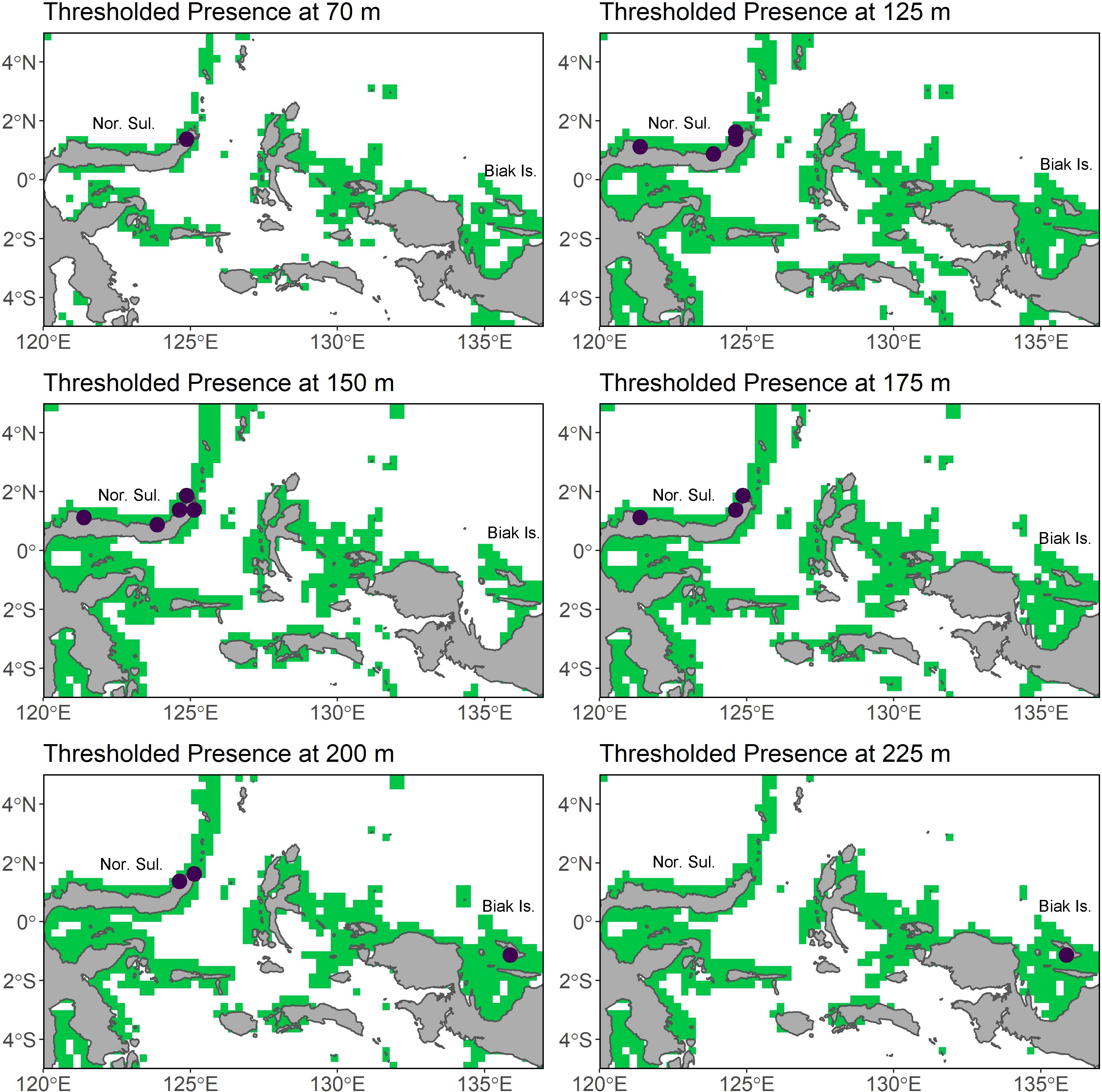
Figure 6. The thresholded 3D model projected into the Indo-Pacific focused over Sulawesi and Biak at each depth slice where an L. menadoensis occurrence has been recorded. Green indicates areas of predicted presence at the 0.8 sensitivity value, and the purple points are recorded L. menadoensis presences. Labels include abbreviations for Northern Sulawesi and Biak Island.
When projected into the habitat of L. menadoensis, the 2D model failed to predict any of the species’ recorded presences except at the 0.99 threshold, where it still omitted 33% of occurrences (Table 1). By contrast, the 3D model counts every L. menadoensis record as a presence, regardless of threshold value. A MESS analysis conducted between the study area in the Mozambique channel and the Indo-Pacific found little environmental difference on a per depth slice basis, suggesting a low risk of extrapolation (Supplementary Figures 3, 4).
A key result of our work is that the 2D vs 3D analyses were strikingly different, showing that the depth at which environmental variables are drawn for a given presence greatly impacts model output. Owens and Rahbek (2023) also found similar outcomes using a different approach, building models focused on surface, benthos or across depths. Our analysis averaged environmental variables from the surface down to the 800 m accessible buffer depth, and 2D and 3D model outputs still disagreed. While it’s plausible that averaging data across depths or relying only on surface or benthos values may not create such a discrepancy for a species whose depth range is greatly restricted or across an environment which is fairly homogeneous by depth, this presents a problem when using 2D ENMs for species with a wider depth preference or which vertically migrate, like the coelacanth. One should note that in the case of the coelacanth, these species appear to be associated with steep slope regions of the benthos. It is therefore possible that a 2D ENM using information from the bottom at a very fine resolution could also capture niche characteristics. However, such 2D environmental data that is presently available is too coarse to capture environmental changes with depth along a steep slope. In general, given these limitations, we anticipate that determining distributions for species more associated with the seabed may still benefit from 3D modelling.
In addition to the lack of agreement between model types, the 2D model performed worse than the 3D one, failing to predict any L. menadoensis presence in the Indo-Pacific, except at the most forgiving threshold value (Figure 7), compared to the latter’s ability to accurately predict all 17 occurrences, regardless of threshold value (Figure 8). This suggests that, in the case of the coelacanths, using the full depth range of a species to build an ENM and projecting that ENM back into 3 dimensions is essential for determining targeted areas for further sampling of either species. While the above argument assumes a degree of niche conservatism, this is a common assumption for allopatric species, as it is a species’ inability to adapt to new environmental conditions which prevents gene flow after a vicariance event (Wiens, 2004). Further, very little morphological differentiation has been noted in comparative analyses between the two species (Meunier et al., 2008; Holder et al., 1999). The extent of morphological similarity was so great in the years immediately following the L. menadoensis discovery, researchers were uncertain if the two were truly distinct species until their genetic divergence was confirmed (Pouyaud et al., 1999). While a divergence time of 30-40 million years (Inoue et al., 2005) is long enough for significant ecological differentiation to occur, Iwata et al. (2019) observed L. menadoensis in the same 15-20°C temperature range as the L. chalumnae individuals observed by Hissmann et al. (2006) and Fricke et al. (1991) off of South Africa and the Comoros. A spatial analysis of niche equivalency or background similarity could further quantify the degree of niche conservatism between the two species, but such analyses typically rely on ENMs as inputs. Robust infrastructure for constructing three-dimensional ENMs and performing such tests for 3D model outputs would also pave the way for the deployment of such analyses in three-dimensional environments.
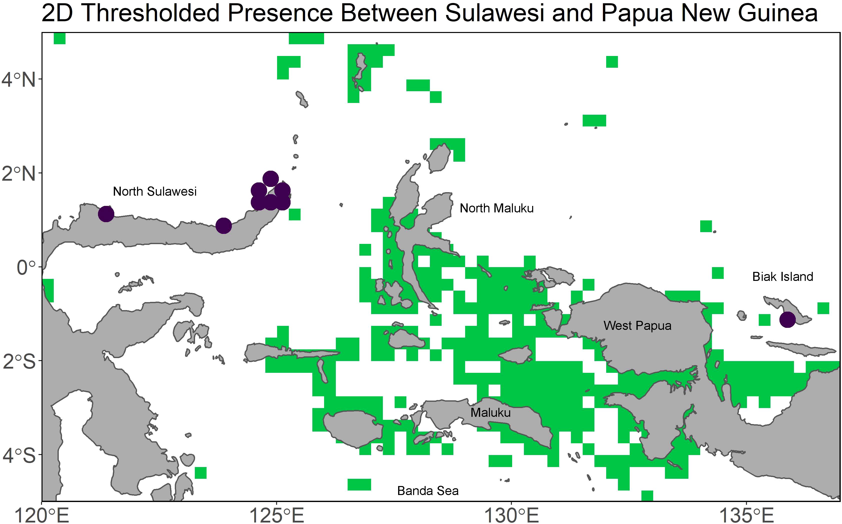
Figure 7. The 2D model projected into the Indo-Pacific and focused over Sulawesi and Biak island. Green indicates areas of predicted presence at the 0.95 sensitivity value, and the purple points are recorded L. menadoensis presences.

Figure 8. A bivariate chloropleth plot of suitable habitat predicted by the 3D L. chalumnae model when projected into the Indo-Pacific.
Further information about L. chalumnae distributions not used in the models above supports the validity of the 3D models. In particular, submersible expeditions off the Comoros between depths of 160 and 550 m (Fricke and Hissmann, 2000) document sightings around caves off the Southwest coast of Grand Comore, where individuals spent the majority of the daytime around volcanic caves between 160 and 250 m. Three large individuals tracked by acoustic transmitters were observed diving up to 550 m at night while hunting (Hissmann et al., 2000). The 3D model also predicts suitable habitat concentrated around the Comoros between 100 and 600 m (Figure 4B). L. chalumnae has also been sighted off the East coast of South Africa in the iSamangaliso Marine Protected Area on three submersible expeditions between 2002 and 2004, notably at depths roughly 100 m shallower than where they are often found in the Comoros (Hissmann et al., 2006). The 3D model predicts some suitability near the marine protected area close to the border with Mozambique at depths between 65 and 275 m, a result consistent with the depth ranges at which L. chalumnae has been observed in that area (Figure 4C). A live coelacanth photographed off the KwaZulu-Natal coast at a depth of 69 m in 2019 seems to support the idea that L. chalumnae has more suitable habitat off of South Africa in shallower waters, possibly because the thermocline separating warm surface waters from colder temperatures occurs at a much shallower depth (Fraser et al., 2020). As can be seen in Figure 4, temperatures do not dip below the coelacanth tolerance limit of 25°C in the Comoros until around 200 m (Figure 4D), while temperatures are already much lower at 50 m off Kwa-Zulu Natal (Figure 4E). The 3D model also predicts suitable habitat off the Southern cape between Capetown and Gqeberha at depths between 60 and 90 m; however, no specimens have ever been recorded that far south perhaps due to dispersal limitations. The 3D model also predicts a fairly consistent line of connectivity from Northern South Africa to Southern Somalia beginning at 100 m and fragmenting at 200 m, suggesting a possible area across which individuals of different African populations could potentially traverse. The model, however, suggests limited connectivity between the African continent, the Comoros, and Madagascar.
Presently, L. menadoensis has only been recorded off of Northern Sulawesi, Biak Island, and off West Papua (Kadarusman et al., 2020). While the model does predict connectivity between Biak and the intervening North Maluku Island beginning at 60 m, there is never a direct line of connectivity between North Sulawesi, North Maluku, and Biak. This raises the question of how the two sighting localities are connected, if at all - it is of course possible that the Sulawesi and Biak individuals belong to disjunct populations. An indirect ring of connectivity does form between Sulawesi and Biak through the islands of the Banda Sea at around 100 m, and this also connects to suitable habitat around the Lesser Sunda Islands and the Philippines. The islands of the Philippines from Luzon to Mindanao are predicted to host Coelacanth suitable habitat largely between 100 - 250 m and remains connected to Sulawesi throughout that depth range. The line of connectivity at this depth range even extends to the Western coast of Indonesia, again via the Banda Sea, as well as along the Northern Coasts of Papua and Papua New Guinea (Figure 6). Considering there is a very well-known ring of volcanic activity from West Sumatra to the Bismarck archipelago, as well as along the Lesser Sunda Islands where the Eurasian plate meets the Australian plate (Figure 9A), it is possible that the volcanic caves coelacanths prefer as daytime shelter are present in these areas of predicted suitability. The majority of suitable habitat is between 100 and 250 m (Figure 9B), and though the preferred temperature conditions of the coelacanth are restricted to a much narrower depth range in this area than in the Comores, between 75 and 250 m (Figure 9C), it is nonetheless habitable in the depth slices where the model predicts suitability. Given the predicted connectivity at the 100 - 250 m depth range and the relative proximity to North Sulawesi and Biak, these areas seem to be the most plausible localities in which to search for possible L. menadoensis populations.
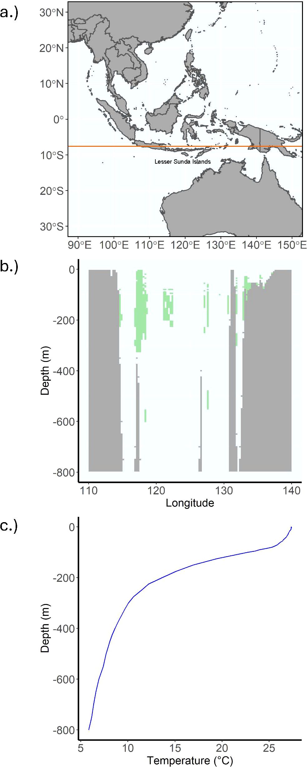
Figure 9. An example of L. chalumnae suitable habitat projected onto the Indo-Pacific. (A) is a map of the area of interest from Southeast Asia to Australia, where the orange line at latitude -7.625 corresponds to the following two plots. (B) depicts L. chalumnae suitable habitat by depth thresholded at the 0.8 sensitivity value in green, while grey corresponds to land or benthos. (C) is a plot of temperature by depth at a given longitude. The thermocline begins around 75 m, and suitable temperature conditions appear to drop off between 200 and 300 m, resulting in a shallower depth range than can be seen in the Comoros.
3D ENM is not without its challenges with regard to both calibration and validation. One particular issue is the greatly increased background compared to traditional 2D models. On the plus side, increased background often provides a broader set of environments for sampling, which can help model calibration. However, this greater background means that diagnostic metrics such as true skill scores converge towards sensitivity, thus weakening the metric’s discriminatory power (Wunderlich et al., 2019). This should be taken into account both during thresholding and model evaluation, either by appropriately adjusting TSS, or perhaps by using a metric more robust to changes in background size. Freer et al. (2020) used AUC, AICc, and TSS in order to quantify performance between 2D and 3D models, and while in their case they concluded that 2D modelling performed best, one should be wary about the applicability of these metrics when comparing the two modelling types. Additionally, AUC is context dependent to the input data of the model due to the representativeness effect (Jiménez-Valverde, 2022). For the same model, AUC can differ depending on how suitability values are distributed, which will likely differ between 2D and 3D. While AUC may inform performance between models trained and tested on the same data, it is not advisable as a discrimination metric between models trained on different datasets, as is the case when comparing 2D and 3D models.
While incorporating the depth axis into ENM construction and projection clearly enhances predictive success compared to traditional 2D modelling, the accuracy of these models could be further augmented by incorporating information relating to physiological and demographic processes. In particular, coelacanths are not able to survive in high water temperatures, are reliant on caves, and have low dispersal ability. Mechanistic or process-oriented modelling involving physiological and dispersal parameters may be necessary for more accurate predictions of potential new coelacanth populations, though these techniques also often require data which at present may be incomplete, especially at depth in marine systems. Depth-structured eDNA sampling would also be a useful supplement for such models, as the quick deterioration rate of eDNA in marine environments is advantageous to species detection (McCartin et al., 2022). Oliver et al. (2024) developed coelacanth specific primers which successfully detected coelacanth eDNA south of Jesser canyon in the iSamangaliso marine protected area. Seeing as these primers can amplify both species while excluding non-coelacanth fish, they could be deployed in areas predicted to be suitable by 3D ENMs as independent model validation.
ENMs which incorporate depth are necessary to make accurate predictions of suitable habitat in marine environments for species like the coelacanth. While traditional 2D models may be viable for species with restricted depth ranges, one is unlikely to accurately capture the suitable habitat of species with wide depth distributions without accounting for environmental variability along the vertical axis. Enhanced scale resolution of environmental data at the bottom may correct this issue for species like the coelacanth which inhabit steep slopes, but this kind of precision is not currently available. It is subsequently vital that infrastructure exists to investigate and project species distributions in the third dimension to properly understand marine community dynamics, patterns of biodiversity, biogeography and speciation, and areas of conservation concern. This infrastructure will become increasingly relevant as commercial operations expand into the deep sea and conservationists reevaluate how reserves are delimited regarding depth (Jacquemont et al., 2024). As in the case of L. chalumnae and L. menadoensis, 3D modelling can give us a more detailed and accurate idea of where to look for further occurrences, as well as what areas may be of conservation interest.
Publicly available datasets were analyzed in this study. This data can be found here: L. chalumnae inventory: https://biostor.org/reference/239560 L. menadoensis field survey: https://doi.org/10.34522/kmnh.17.0_49 NOAA WOA: https://www.ncei.noaa.gov/access/world-ocean-atlas-2018/ ETOPO global relief model: https://www.ncei.noaa.gov/products/etopo-global-relief-model Copernicus Marine Service Global Ocean Physics Analysis and Forecast: https://data.marine.copernicus.eu/product/GLOBAL_ANALYSISFORECAST_PHY_001_024/description.
ES: Conceptualization, Data curation, Formal analysis, Investigation, Methodology, Software, Validation, Visualization, Writing – original draft. HO: Conceptualization, Methodology, Software, Writing – review & editing. RG: Conceptualization, Data curation, Funding acquisition, Methodology, Project administration, Resources, Supervision, Writing – review & editing. GN: Conceptualization, Funding acquisition, Project administration, Resources, Supervision, Writing – review & editing.
The author(s) declare financial support was received for the research, authorship, and/or publication of this article. HO was supported under research grant no. 25925 from Villum Fonden.
Emaline Sheahan acknowledges support provided by a Graduate Research Fellowship from the University of Florida. We would also like to thank the Guralnick and Naylor labs for providing input on the project.
The authors declare that the research was conducted in the absence of any commercial or financial relationships that could be construed as a potential conflict of interest.
The author(s) declared that they were an editorial board member of Frontiers, at the time of submission. This had no impact on the peer review process and the final decision.
The author(s) declare that no Generative AI was used in the creation of this manuscript.
All claims expressed in this article are solely those of the authors and do not necessarily represent those of their affiliated organizations, or those of the publisher, the editors and the reviewers. Any product that may be evaluated in this article, or claim that may be made by its manufacturer, is not guaranteed or endorsed by the publisher.
The Supplementary Material for this article can be found online at: https://www.frontiersin.org/articles/10.3389/fmars.2025.1521474/full#supplementary-material
Abbott J. C., Bota-Sierra C. A., Guralnick R., Kalkman V., González-Soriano E., Novelo-Gutiérrez R., et al. (2022). Diversity of nearctic dragonflies and damselflies (Odonata). Diversity. 14, 575. doi: 10.3390/d14070575
Aiello-Lammens M. E., Boria R. A., Radosavljevic A., Vilela B. (2015). spThin: an R package for spatial thinning of species occurrence records for use in ecological niche models. Ecography. 38, 541–545. doi: 10.1111/ecog.2015.v38.i5
Allouche O., Tsoar A., Kadmon R. (2006). Assessing the accuracy of species distribution models: prevalence, kappa and the true skill statistic (TSS). J. Appl. Ecol. 43, 1223–1232. doi: 10.1111/j.1365-2664.2006.01214.x
Amante C., Eakins B. W. (2009). ETOPO1 1 Arc-Minute Global Relief Model: Procedures, Data Sources and Analysis. NOAA Technical Memorandum NESDIS NGDC-24 (Colorado: National Geophysical Data Center, NOAA). doi: 10.7289/V5C8276M
Bentlage B., Peterson A. T., Barve N., Cartwright P. (2013). Plumbing the depths: extending ecological niche modelling and species distribution modelling in three dimensions. Global Ecol. Biogeogr. 22, 952–961. doi: 10.1111/geb.2013.22.issue-8
Boyer T. P., Baranova O. K., Coleman C., Garcia H. E., Grodsky A., Locarnini R. A., et al. (2019). World Ocean Database 2018. Ed. Mishonov A. (Silver Spring, Maryland: NOAA Atlas NESDIS), 87.
Clement A. M., Cloutier R., Lee M. S. Y., King B., Vanhaesebroucke O., Bradshaw C. J. A., et al. (2024). A Late Devonian coelacanth reconfigures actinistian phylogeny, disparity, and evolutionary dynamics. Nat. Commun. 15, 7529. doi: 10.1038/s41467-024-51238-4
Cooke A., Bruton M. N., Ravololoharinjara M. (2021). Coelacanth discoveries in Madagascar, with recommendations on research and conservation. S. Afr. J. Sci. 117, 3–4. doi: 10.17159/sajs.2021/8541
Coro G., Pagano P., Ellenbroek A. (2013). ). Combining simulated expert knowledge with Neural Networks to produce Ecological Niche Models for Latimeria chalumnae. Ecol. Model. 268, 55–63. doi: 10.1016/j.ecolmodel.2013.08.005
Erdmann M. V. (1998). An account of the first living coelacanth known to scientists from Indonesian waters. Environ. Biol. Fishes. 54, 439–443. doi: 10.1023/A:1007584227315
Fraser M. D., Henderson B. A. S., Carstens P. B., Fraser A. D., Henderson B. S., Dukes M. D., et al. (2020). Live coelacanth discovered off the KwaZulu-Natal South Coast, South Africa. S Afr J. Sci. 116, 7806. doi: 10.17159/sajs.2020/7806
Freer J. J., Tarling G. A., Collins M. A., Partridge J. C., Genner M. J. (2020). Estimating circumpolar distributions of lanternfish using 2D and 3D ecological niche models. Mar. Ecol. Prog. Ser. 647, 179–193. doi: 10.3354/meps13384
Fricke H., Hissmann K. (2000). Feeding ecology and evolutionary survival of the living coelacanth Latimeria chalumnae. Mar. Biol. 136, 379–386. doi: 10.1007/s002270050697
Fricke H., Hissmann K., Froese R., Schauer J., Plante R., Fricke S. (2011). The population biology of the living coelacanth studied over 21 years. Mar. Biol. 158, 1511–1522. doi: 10.1007/s00227-011-1667-x
Fricke H., Schauer J., Hissmann K., Kasang L., Plante R. (1991). Coelacanth Latimeria chalumnae aggregates in caves: first observations on their resting habitat and social behavior. Environ. Biol. Fishes. 30, 281–285. doi: 10.1007/BF02028843
Froese R., Palomares M. L. D. (2000). Growth, natural mortality, length–weight relationship, maximum length and length-at-first-maturity of the coelacanth Latimeria chalumnae. Environ. Biol. Fishes. 58, 45–52. doi: 10.1023/A:1007602613607
Garcia H. E., Weathers K. W., Paver C. R., Smolyar I. V., Boyer T. P., Locarnini R. A., et al. (2019a). World Ocean Atlas 2018, Volume 3: Dissolved Oxygen, Apparent Oxygen Utilization, and Oxygen Saturation. Ed. Mishonov A. (Silver Spring, Maryland: NOAA Atlas NESDIS), 83.
Garcia H. E., Weathers K. W., Paver C. R., Smolyar I. V., Boyer T. P., Locarnini R. A., et al. (2019b). World Ocean Atlas 2018, Volume 4: Dissolved Inorganic Nutrients (phosphate, nitrate, silicate). Ed. Mishonov A. (Silver Spring, Maryland: NOAA Atlas NESDIS), 84.
Hijmans R. (2024). terra: Spatial Data Analysis. R package version 1. Available online at: https://github.com/rspatial/terra (Accessed October 13, 2024).
Hissmann K., Fricke H., Schauer J. (2000). Patterns of time and space utilisation in coelacanths (Latimeria chalumnae), determined by ultrasonic telemetry. Mar. Biol. 136, 943–952. doi: 10.1007/s002270000294
Hissmann K., Fricke H., Schauer J., Ribbink A. J., Roberts M., Sink K., et al. (2006). The South African coelacanths - an account of what is known after three submersible expeditions. S. Afr. J. Sci. 102, 491–500. doi: https://hdl.handle.net/10520/EJC96593
Holder M. T., Erdmann M. V., Wilcox T. P., Caldwell R. L., Hillis D. M. (1999). Two living species of coelacanths? Proc. Natl. Acad. Sci. 96, 12616–12620. doi: 10.1073/pnas.96.22.12616
Inoue J. G., Miya M., Venkatesh B., Nishida M. (2005). The mitochondrial genome of Indonesian coelacanth Latimeria menadoensis (Sarcopterygii: Coelacanthiformes) and divergence time estimation between the two coelacanths. Gene. 349, 227–235. doi: 10.1016/j.gene.2005.01.008
Iwata M., Yabumoto Y., Saruwatari T., Yamauchi S., Fujii K., Ishii R., et al. (2019). Field surveys on the Indonesian coelacanth, Latimeria menadoensis using remotely operated vehicles from 2005 to 2015. Bull. Kitakyushu Mus. Nat. Hist. Hum. Hist. Ser. A. 17, 49–56. doi: 10.34522/kmnh.17.0_49
Jacquemont J., Loiseau C., Tornabene L., Claudet J. (2024). 3D ocean assessments reveal that fisheries reach deep but marine protection remains shallow. Nat. Commun. 15, 4027. doi: 10.1038/s41467-024-47975-1
Jiménez-Valverde A. (2022). The uniform AUC: Dealing with the representativeness effect in presence–absence models. Methods Ecol. Evol. 13, 1224–1236. doi: 10.1111/2041-210X.13826
Johanson Z., Long J. A., Talent J. A., Janvier P., Warren J. W. (2006). Oldest coelacanth, from the early devonian of Australia. Biol. Lett. 2, 443–446. doi: 10.1098/rsbl.2006.0470
Kadarusman, Sugeha H. Y., Pouyaud L., Hocde R., Hismayasari I. B., Gunaisah E., et al. (2020). A thirteen-million-year divergence between two lineages of Indonesian coelacanths. Sci. Rep. 10, 192. doi: 10.1038/s41598-019-57042-1
Kass J. M., Muscarella R., Galante P. J., Bohl C. L., Pinilla-Buitrago G. E., Boria R. A., et al. (2021). ENMeval 2.0: Redesigned for customizable and reproducible modeling of species’ niches and distributions. Methods Ecol. Evol. 12, 1602–1608. doi: 10.1111/2041-210X.13628
Lampert K. P., Fricke H., Hissmann K., Schauer J., Blassmann K., Ngatunga B. P., et al. (2012). Population divergence in East African coelacanths. Curr. Biol. 22, PR439–PR440. doi: 10.1016/j.cub.2012.04.053
Locarnini R. A., Mishonov A. V., Baranova O. K., Boyer T. P., Zweng M. M., Garcia H. E., et al. (2019a). World Ocean Atlas 2018, Volume 1: Temperature. Ed. Mishonov A. (Silver Spring, Maryland: NOAA Atlas NESDIS), 81.
Locarnini R. A., Zweng M. M., Mishonov A. V., Baranova O. K., Reagan J. R., Seidov D., et al. (2019b). World Ocean Atlas 2018, Volume 5: In situ Density. Ed. Mishonov A. (Silver Spring, Maryland: NOAA Atlas NESDIS), 85.
McCartin L. J., Vohsen S. A., Ambrose S. W., Layden M., McFadden C. S., Cordes E. E., et al. (2022). Temperature Controls eDNA Persistence across Physicochemical Conditions in Seawater. Environ. Sci. Technol. 56, 8629–8639. doi: 10.1021/acs.est.2c01672
Melo-Merino S. M., Reyes-Bonilla H., Lira-Noriega A. (2020). Ecological niche models and species distribution models in marine environments: A literature review and spatial analysis of evidence. Ecol. Model. 415, 108837. doi: 10.1016/j.ecolmodel.2019.108837
Meunier F. J., Erdmann M. V., Fermon Y., Caldwell R. L. (2008). Can the comparative study of the morphology and histology of the scales of Latimeria menadoensis and L. chalumnae (Sarcopterygii: Actinistia, Coelacanthidae) bring new insight on the taxonomy and the biogeography of recent coelacanthids? Geol. Soc Spec. Publ. 295, 351–360. doi: 10.1144/SP295.17
Nulens R., Scott L., Herbin M. (2011). An updated inventory of all known specimens of the coelacanth, Latimeria spp. Smithiana Spec. Publ 3, 1–52.
Oliver J. C., Shum P., Mariani S., Sink K. J., Palmer R., Matcher G. F. (2024). Enhancing African coelacanth monitoring using environmental DNA. Biol. Lett. 20, 20240415. doi: 10.1098/rsbl.2024.0415
Owens H., Bentley A. C., Peterson A. T. (2012). Predicting suitable environments and potential occurrences for coelacanths (Latimeria spp.). Biodivers Conserv. 21, 577–587. doi: 10.1007/s10531-011-0202-1
Owens H., Rahbek C. (2023). voluModel: Modelling species distributions in three-dimensional space. Methods Ecol. Evol. 14, 841–847. doi: 10.1111/2041-210X.14064
Phillips S. J., Anderson R. P., Schapire R. E. (2006). Maximum entropy modeling of species geographic distributions. Ecol. Modell. 190, 231–259. doi: 10.1016/j.ecolmodel.2005.03.026
Pouyaud L., Wirjoatmodjo S., Rachmatika I., Tjakrawidjaja A., Hadiaty R., Hadie W. (1999). A new species of coelacanth. Genetic and morphological evidence. C. R. Acad. Sci. III. 322, 261–267. doi: 10.1016/S0764-4469(99)80061-4
Reagan J. R., Zweng M. M., Locarnini R. A., Seidov D., Mishonov A. V., Baranova O. K., et al. (2019). World Ocean Atlas 2018, Volume 6: Ocean Conductivity. Ed. Mishonov A. (Silver Spring, Maryland: NOAA Atlas NESDIS), 86.
Sillero N., Barbosa A. M. (2021). Common mistakes in ecological niche models. Int. J. Geogr. Inf. Sci. 35, 213–226. doi: 10.1080/13658816.2020.1798968
Wiens J. J. (2004). Speciation and ecology revisited: phylogenetic niche conservatism and the origin of species. Evolution. 58, 193–197. doi: 10.1111/j.0014-3820.2004.tb01586.x
Wunderlich R. F., Lin Y., Anthony J., Petway J. R. (2019). Two alternative evaluation metrics to replace the true skill statistic in the assessment of species distribution models. Nat. Conserv. 35, 97–116. doi: 10.3897/natureconservation.35.33918
Keywords: ecological niche models, coelacanth, 3D, 2D, species distribution
Citation: Sheahan E, Owens H, Guralnick R and Naylor G (2025) 3D ecological niche models outperform 2D in predicting coelacanth (Latimeria spp.) habitat. Front. Mar. Sci. 12:1521474. doi: 10.3389/fmars.2025.1521474
Received: 01 November 2024; Accepted: 03 February 2025;
Published: 06 March 2025.
Edited by:
Lionel Cavin, Natural History Museum of Geneva, SwitzerlandReviewed by:
Matteo Zucchetta, National Research Council (CNR), ItalyCopyright © 2025 Sheahan, Owens, Guralnick and Naylor. This is an open-access article distributed under the terms of the Creative Commons Attribution License (CC BY). The use, distribution or reproduction in other forums is permitted, provided the original author(s) and the copyright owner(s) are credited and that the original publication in this journal is cited, in accordance with accepted academic practice. No use, distribution or reproduction is permitted which does not comply with these terms.
*Correspondence: Emmaline Sheahan, c2hlYWhhbmVAdWZsLmVkdQ==
†These authors share last authorship
Disclaimer: All claims expressed in this article are solely those of the authors and do not necessarily represent those of their affiliated organizations, or those of the publisher, the editors and the reviewers. Any product that may be evaluated in this article or claim that may be made by its manufacturer is not guaranteed or endorsed by the publisher.
Research integrity at Frontiers
Learn more about the work of our research integrity team to safeguard the quality of each article we publish.