Antarctic krill habitat suitability variation in the Southern Ocean over 20 years

Antarctic krill (Euphausia superba) is a key species that sustains the biodiversity of the Southern Ocean and is a protected and restricted fishing target in this region. Considering the significant impacts of climate change on the ecological environment of the Southern Ocean, it is critical to understand the long-term spatio-temporal habitat distribution of Antarctic krill. This study integrates remote sensing and reanalysis data with Antarctic krill survey records to evaluate krill habitat suitability in the Southern Ocean. A novel habitat suitability model was developed using phytoplankton phenology and sea ice dynamics as key timing parameters, employing the Categorical Boosting (CatBoost) algorithm. This is the first time interannual variation in krill habitat distribution, spanning over 20 years (1997–2019), has been analyzed in relation to environmental parameters. Results show that the ice-free period in the Amundsen Sea has extended annually, while phytoplankton blooms have occurred earlier, lasted longer, and exhibited increasing chlorophyll a concentration (CHL), particularly in coastal regions. Additionally, the CatBoost model outperformed traditional species distribution models (SDMs) in handling large-scale presence-absence data (GCV = 0.16), demonstrating that bloom peak CHL and sea ice retreat timing are more effective indicators of krill habitat suitability than single-time environmental parameters. Based on long-term changes in highly suitable habitat areas for Antarctic krill and synchronized trends with the Southern Annular Mode (SAM) index, the overall area of suitable habitat for Antarctic krill in the Prydz sector has declined, likely linked to surface cooling caused by climate change. In contrast, the coastal region of the Atlantic sector, particularly the Western Antarctic Peninsula, a rapid warming area, has experienced an increase in krill habitat suitability. However, habitat suitability in the Weddell Sea has shown a marked decrease. Although climate change has produced mixed effects on krill habitats due to the varying responses of krill different life stages to environmental parameters, this study overall highlights a degradation of krill habitat in the Southern Ocean over the past two decades. These findings provide new insights into Antarctic krill habitat modeling and offer a long-term perspective on the climate change impacts, emphasizing the need for future under-ice investigations.

1 Introduction

Antarctic krill (Euphausia superba) is a small, pelagic crustacean inhabiting the Southern Ocean, known for its enormous biomass, which plays a crucial role in sustaining the Southern Ocean food web and biodiversity (Croxall et al., 1999; Trathan and Hill, 2016). By feeding on large amounts of phytoplankton and conducting diel vertical migrations, Antarctic krill accelerates the downward export and transport of particles, thereby promoting marine biogeochemical cycles (Cavan et al., 2019). Krill are also sensitive to climate and environmental changes, serving as an indicator species for the fragile habitat of the Southern Ocean. For instance, increasing CO₂ concentrations, rising temperatures, and sea ice melting can trigger responses in krill related to egg hatching, spatial distribution, and abundance (Kawaguchi et al., 2013). Antarctic krill is a major food source for Southern Ocean predators (Croxall et al., 1999; Trathan and Hill, 2016) and an important target for commercial fisheries (Meyer et al., 2020). To preserve the biodiversity of the Southern Ocean ecosystem, the Commission for the Conservation of Antarctic Marine Living Resources (CCAMLR) has designated Antarctic krill as a key species under protection and introduced precautionary fishing limits (Siegel, 2016). Therefore, in light of the significant ongoing changes in the Southern Ocean’s ecological environment, it is critical to assess the spatio-temporal distribution, trends, and habitat suitability of Antarctic krill.

Numerous studies have used environmental parameters derived from remote sensing and reanalysis models, in combination with krill population growth models, to predict habitat growth potential for Antarctic krill (Piñones and Fedorov, 2016) and assess habitat suitability in the Southern Ocean. Thorpe et al. (2019) developed a krill growth model for juveniles based on bathymetry, sea temperature, and sea ice concentration (SIC) data, finding that krill population growth in some nearshore areas is constrained by sea ice. Atkinson et al. (2006) incorporated remotely sensed chlorophyll concentrations (CHL) and sea surface temperature (SST) into a krill growth model, showing that remotely sensed CHL significantly improves the accuracy of daily krill growth rate predictions. Flores et al. (2012b) used mixed-layer depth (MLD) and related vertical profile parameters in a krill juvenile density prediction model, finding a positive correlation between juvenile krill density and MLD during the Antarctic summer when MLD is less than 12 m or ranges between 20-30 m. While these studies elucidate the relationships between Antarctic krill and environmental parameters, they lack discussions on the indicative role of temporal characteristics in habitat suitability. Some studies have explored the relationship between krill recruitment and sea ice phenology in the southwest Atlantic based on SIC-derived sea ice growth and retreat timing (Veytia et al., 2021), while others have provided distributions and trends of phytoplankton bloom phenological parameters in the Southern Ocean (Thomalla et al., 2023). These studies offer potential timing parameters for Antarctic krill habitat suitability models and phenological feature extraction.

The modeling and assessment of Antarctic krill habitat suitability are generally based on species distribution models (SDMs), including linear mixed models (LMM) (Kawaguchi et al., 2006; Brown et al., 2010; Candy, 2021), generalized additive models (GAMs) (Trathan et al., 2003; Murase et al., 2013; Trathan et al., 2022), and the maximum entropy model (Maxent) (Friedlaender et al., 2011; Nachtsheim et al., 2017; Lin et al., 2022), all of which have been applied in studies on krill distribution. These models have shown promising predictive and assessment outcomes, but their applicability and generalizability still require further improvement. Traditional SDM models, for instance, lack the ability to handle missing data, which is a common issue for environmental parameters such as CHL. And the missing data in CHL is in relation to krill density, as krill swarms could lead to zero values. Additionally, SDM models are subject to various limitations. Maxent, for example, is better suited for small presence-only datasets and is sensitive to spatial sampling bias and model complexity, which can result in prediction errors (Taylor et al., 2020; Lin et al., 2022). In this context, CatBoost (Categorical Boosting), a model capable of handling missing data, emerges as a suitable alternative. CatBoost is a gradient boosting framework, which is an ensemble learning technique that combines multiple decision trees to create a strong predictive model (Prokhorenkova et al., 2018). CatBoost automatically handles missing values in the input data by treating missing values as a separate category and learning a specific pattern for them during the training process. This approach allows CatBoost to capture the relationship between the missing values and the target variable, which can be particularly useful when the missingness itself carries important information. Therefore, CatBoost offers a novel approach for modeling the Antarctic krill habitat in the Southern Ocean, particularly under conditions where environmental variables are complex and contain missing values. Additionally, it addresses the issue of insufficient dataset matching that hampers larger-scale fitting. However, the application of CatBoost in species distribution modeling is still relatively limited.

Antarctic krill have a wide circum-Antarctic distribution, and their responses and adaptations to environmental changes are complex. Consequently, the response characteristics and mechanisms of krill distribution to environmental factors vary across different spatial and temporal scales. Existing studies have mainly focused on the Antarctic Peninsula and Scotia Sea in the western Southern Ocean, with relatively few studies evaluating habitat suitability in East Antarctica (Bibik et al., 1988; Lin et al., 2022). Research on the habitat suitability of Antarctic krill across the entire Southern Ocean primarily focuses on krill recruitment and their future responses to climate change, lacking historical reviews of krill habitat changes (Veytia et al., 2020). Moreover, few studies have assessed the spatio-temporal distribution of Antarctic krill habitat suitability based on long-term time series data (Candy, 2021).

This study, focusing on the entire Southern Ocean (45°S–90°S), integrates field observations and long-term remote sensing and reanalysis datasets spanning more than 20 years (1997-2019) at daily and 8-day averages. It introduces temporal parameters related to phytoplankton bloom phenology and sea ice dynamics to construct a krill habitat suitability model using the CatBoost algorithm. The study explores the relationship between krill spatial distribution and environmental factors through a systematic comparison of four sectors: the Atlantic sector, Lazarev sector, Prydz sector, and Ross sector, identifying similarities and differences in the spatio-temporal variation of krill and its interactions with the marine ecological environment.

2 Data and methods

2.1 Study region and survey data

The study area is located in the Southern Ocean, covering the region between 45°S and 90°S surrounding Antarctica. To investigate the regional differences and characteristics of Antarctic krill habitat suitability across various sectors of the Southern Ocean, the study area was divided into 4 sectors (Yang et al., 2021): Atlantic sector (90°W–10°W), Lazarev sector (10°W–60°E), Prydz sector (60°E–150°E), and Ross sector (150°E–90°W) (Figure 1A).

Figure 1

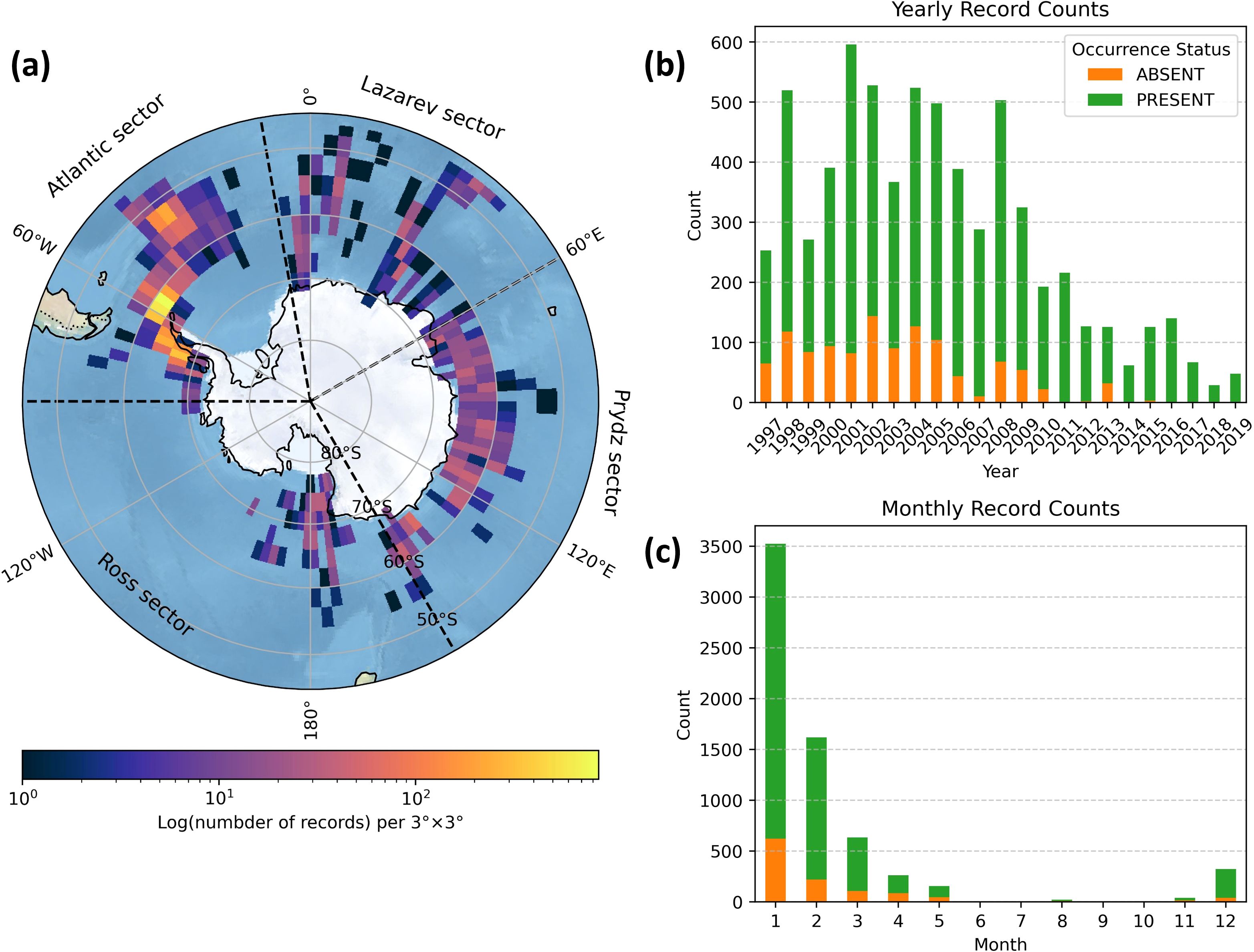
Figure 1. Antarctic krill survey data (A) density and Atlantic sector, Lazarev sector, Prydz sector, and Ross sector in the study region, and number of Antarctic krill survey records for (B) each year and (C) each month.

The Antarctic krill data used in this study were sourced from the Global Biodiversity Information Facility (GBIF, https://www.gbif.org/) database on Euphausia superba Dana, 1850. Based on the raw dataset from GBIF, we conducted a validation and filtering process. First, we restricted the dataset to records from 1997 to 2020 and excluded entries lacking date information, including those record flagged as “record date unlikely” and “record date mismatch.” Second, we retained only those records that contained latitude and longitude information, specifically within the latitude from 45°S to 90° S. Notably, some records were missing the negative sign for latitude; we corrected these by adding negative sign before retention. Next, we filtered the dataset to remove those data that were not derived from standardized observations (including acoustic and trawling investigation) or identified institutions (e.g. individual user-verified records from iNaturalist). We also examined the data source to exclude datasets that are not in situ observations, such as those related to stomach contents. We verified original source for each record to ensure the records pertained to Antarctic krill to avoid incorrect classification in GBIF. Finally, we removed duplicate records by merging them with identical dates and coordinates into a single one, retaining presence as occurrence status when both presence and absence data appear. Dataset after standardization is provided in the Supplementary Material (Supplementary Table 1).

Standardized dataset is composed of 12 original datasets and contains a total of 6,603 presence-absence records of Antarctic krill, with their distribution density across the Southern Ocean illustrated in Figure 1. Among these, there are 5,444 presence records and 1,143 absence records. The majority of the survey datasets present adult krill as dominant, with other life stages representing a smaller proportion. The sharp decline in the number of krill surveys after 2010 primarily stems from CCAMLR’s restrictions on Antarctic krill fishing (CCAMLR, 2008) (Figure 1B). Given that Antarctic krill migrate to surface waters during the Austral summer, making them easier to observe, this study focuses on the habitat suitability of Antarctic krill from November to April, during which 97.2% of the krill survey data were collected (Figure 1C).

2.2 Remote sensing data and reanalysis data

The remote sensing and reanalysis data used in this study are listed in Table 1. Sea surface temperature (SST) data were obtained from the Level 4 product of the Group for High-Resolution Sea Surface Temperature (GHRSST) dataset. This gridded product is derived from satellite, ship, and buoy observations, with the remote sensing data primarily sourced from the optimally interpolated global SST product based on the Advanced Very High-Resolution Radiometer (AVHRR) (Huang et al., 2021). The data are available at https://www.ncei.noaa.gov/data/sea-surface-temperature-optimum-interpolation.

Table 1

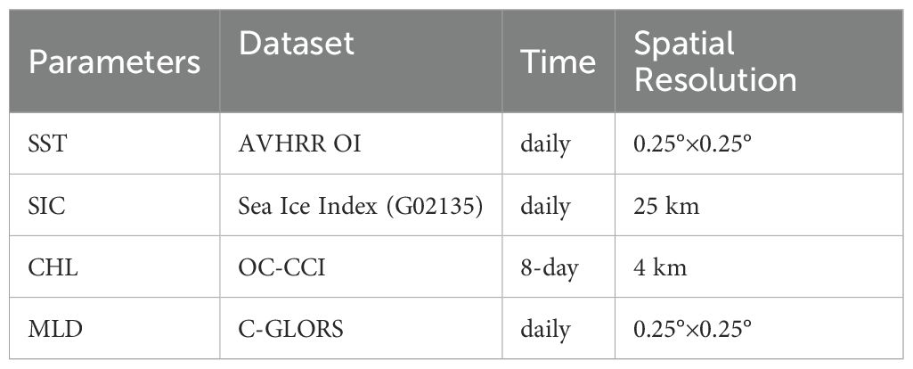
Table 1. Summary information of remote sensing data and reanalysis data used in this study.

Sea ice concentration (SIC) data were sourced from the National Snow and Ice Data Center (NSIDC). These data are obtained from observations by the Defense Meteorological Satellite Program (DMSP) and the Nimbus-7 satellite platform (Fetterer et al., 2017). Daily SIC products can be accessed at https://noaadata.apps.nsidc.org/NOAA/G02135/, and the product also provides the date of the minimum annual sea ice extent.

Sea surface chlorophyll concentration (CHL) data were obtained from the Ocean Colour Climate Change Initiative (OC-CCI), developed by the European Space Agency (ESA) Climate Change Initiative. This reanalysis dataset (version 5.0) integrates multi-sensor satellite observations, including data from MERIS, MODIS Aqua, Sentinel-3 OLC, SeaWiFS, and VIIRS, and is available at https://www.oceancolour.org/ (Sathyendranath et al., 2021). Due to significant interference from sea ice cover and clouds, there are substantial gaps in the ocean color data. To address this, we employed the gap-filling method developed by Thomalla et al. (2023) for the OC-CCI CHL product.

Mixed-layer depth (MLD) data were derived from the CMCC Global Ocean Physical Reanalysis System (C-GLORS) dataset. This dataset is produced using the NEMO ocean model coupled with the LIM2 sea ice model and calculated via the OceanVar data assimilation system (Storto and Masina, 2016). The data can be accessed at https://data.marine.copernicus.eu/product/.

2.3 Timing parameters of phytoplankton bloom and sea ice dynamics

2.3.1 Phytoplankton bloom timing parameters

Phytoplankton blooms refer to the rapid proliferation and accumulation of phytoplankton, during which chlorophyll-a (CHL) concentrations increase significantly. Previous studies have shown that bloom phenology can affect fishery yields. For instance, variations in the timing and duration of spring blooms are closely correlated with the survival and development of juvenile fish (Platt et al., 2003). Antarctic krill larvae exhibit similar characteristics in population growth models (Kohlbach et al., 2017). Bloom phenology parameters include the onset and termination dates within a year, the bloom peak, and its duration, among others (Thomalla et al., 2023). In this study, we used Antarctic krill occurrence records and the corresponding CHL time series to construct bloom phenology parameters and analyze their temporal correlations (i.e., time lags) with krill occurrence. The schematic diagram of the phytoplankton bloom timing parameters is presented in the Supplementary Material (Supplementary Figure 1a). We used the calculation methods from (Ferreira et al., 2022) for the key bloom phenology parameters, which are presented below (Equations 1–7):

$\begin{array}{ll}CH{L}_{BloomThreshold}=(CH{L}_{max}-CH{L}_{min})\times \mathbf{5}\%+CH{L}_{min}& (1)\end{array}$

In Equation 1, $CH{L}_{BloomThreshold}$ (mg·m^-3) was calculated from the maximum ($CH{L}_{max}$, mg·m^-3) and minimum ($CH{L}_{min}$, mg·m^-3) CHL of timeseries during observation period (from July 1 of each year to June 30 of the following year). The 5% threshold was established through research by Siegel et al. (2002), determining a chlorophyll-a concentration level that corresponds just above the median biomass value on the bloom initiation day.

$\begin{array}{ll}{t}_{BloomDur}=t_{BloomTerm}-t_{BloomInit}& (2)\end{array}$

In Equation 2, the bloom duration ($t_{BloomDur}$) is the duration between bloom initiation and termination. The time at which CHL first exceeds the bloom threshold ($CH{L}_{BloomThreshold}$) marks the initiation of the bloom ($t_{BloomInit}$). The bloom termination ($t_{BloomTerm}$) is defined as the time when CHL falls below the bloom threshold after reaching its peak. The peak value of CHL timeseries during bloom ($CH{L}_{\text{BloomPeak}}$) and the time ($t_{\text{BloomPeak}}$) when CHL peaks are identified using the Python function find_peaks, searching for peaks in the CHL time series (${\left\{CH{L}_t\right\}}_{t=1}^T$) during the bloom period. And the parameter “height” limits the minimum value of peak CHL.

$\begin{array}{ll}CH{L}_{BloomInteg}={\displaystyle \sum _{\mathit{i}=\mathbf{1}}^{t_{BloomDur}}CH{L}_i}& (3)\end{array}$

In Equation 3, the cumulative chlorophyll-a concentration during the bloom period is estimated using the trapezoidal rule to integrate CHL during bloom ($CH{L}_{BloomInteg}$).

$\begin{array}{ll}{t}_{DABloomInit}=t_{AKO}-t_{BloomInit}& (4)\end{array}$

$\begin{array}{ll}{t}_{DBBloomTerm}=t_{BloomTerm}-t_{AKO}& (5)\end{array}$

$\begin{array}{ll}{t}_{DBBloomPeak}=t_{BloomPeak}-t_{AKO}& (6)\end{array}$

In Equations 4, 5, to determine the temporal relationship between the phytoplankton bloom and Antarctic krill observations ($t_{AKO}$), the number of days between the krill observation date and the bloom initiation date ($t_{DABloomInit}$) is calculated. “DABloomInit” here refers to days after bloom initiation. This implies that we assume observations of Antarctic krill typically occur during phytoplankton bloom periods, which is consistent with the phenology of the Antarctic krill. Thus, the difference between the krill observation date and the bloom termination date is calculated as $t_{DBBloomTerm}$ referring to days before bloom termination. And the difference between the krill observation and the CHL peak time date is calculated as $t_{DBBloomPeak}$ referring to days before CHL peak time in Equation 6 .

$\begin{array}{ll}CH{L}_{BloomMean}=\frac{CH{L}_{BloomInteg}}{t_{BloomDur}}& (7)\end{array}$

Finally, in Equation 7, $CH{L}_{BloomMean}$ is calculated from $CH{L}_{BloomInteg}$ and $t_{BloomDur}$, representing mean CHL during phytoplankton bloom. The units and definitions of all the phytoplankton bloom timing parameters mentioned above can be found in Table 2.

Table 2

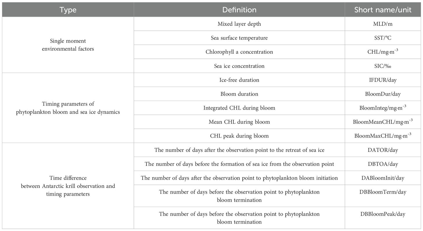
Table 2. Environmental parameters for Antarctic krill survey data.

2.3.2 Sea ice dynamics timing parameters

The sea ice phenology parameters, representing sea ice arrival and retreat, can be calculated from the SIC time series. The sea ice formation time, or time of arrival (TOA), is defined as the date when SIC first reaches or exceeds 15% in a given year; the sea ice retreat time, or time of retreat (TOR), is determined by searching backwards from the date of the minimum sea ice extent in the following year until SIC first reaches or exceeds 15% (Stammerjohn et al., 2008). The schematic diagram of the sea ice dynamics timing parameters is presented in the Supplementary Material (Supplementary Figure 1b). Since the Antarctic krill observations are primarily recorded in ice-free areas, the ice-free duration (IFDUR) is calculated to represent the length of time without sea ice. The time differences between sea ice dynamics and krill observations are calculated as the number of days after sea ice retreat (DATOR), measured as the days between krill occurrence ($t_{AKO}$) and the sea ice retreat time, and the number of days before sea ice formation (DBTOA), calculated as the days between krill occurrence and the sea ice arrival time. The sea ice phenology parameter calculations and their formulas are presented in Equations 8–10:

$\begin{array}{ll}{t}_{IFDUR}=t_{TOA}-t_{TOR}& (8)\end{array}$

$\begin{array}{ll}{t}_{DBTOA}=t_{TOA}-t_{AKO}& (9)\end{array}$

$\begin{array}{ll}{t}_{DATOR}=t_{AKO}-t_{TOR}& (10)\end{array}$

2.4 Suitability model development and validation

In this study, the CatBoost algorithm was used to construct a habitat suitability model for Antarctic krill. The selected parameters were divided into 3 categories: (a) conventional single-moment environmental parameters, (b) sea ice and phytoplankton bloom phenology parameters, and (c) the time differences between krill observations and timing parameters. A total of 14 parameters were selected. Antarctic krill survey records were matched with the 14 environmental data parameters based on latitude, longitude, and date to create a matched dataset. Genuine cross-validation (GCV) was employed to assess the model’s overall performance. This dataset was divided into 2 parts for developing CatBoost model: for each year (starting from July 1st to ensure data continuity), data from that year were excluded for validation, and the remaining data were input for training. The model’s performance is assessed by averaging the accuracy obtained from modeling and validating each year through a leave-one-out approach.

The model’s classification accuracy was evaluated using three metrics: (a) mean squared error (MSE), (b) Area Under the Curve (AUC) of the Receiver Operating Characteristic (ROC), and (c) True Skill Statistic (TSS). Factors with low contribution to the model and strong collinearity will be filtered out for re-modeling in order to identify the optimal model. Additionally, a limitation was imposed on the number of non-null environmental parameters input to reduce the uncertainty in prediction results caused by excessive missing values. The predictive accuracy in different experiments were compared to determine the optimal model for reconstructing Antarctic krill habitat suitability. Finally, since extended daylight during the Austral summer boosts phytoplankton blooms, causing krill to migrate to surface waters, which align with both coverage of our survey records and the focus of our study, the model outputs were limited to the period from November to April of the subsequent year. The model produced daily habitat suitability distributions for Antarctic krill in the Southern Ocean from 1997 to 2019. The entire workflow of the modeling process is illustrated in the Supplementary Material (Supplementary Figure 2).

2.4.1 Matchup dataset for suitability model

Based on the obtained MLD, SST, SIC, and gap-filled CHL products, along with the calculated timing parameters for phytoplankton bloom and sea ice dynamics, the corresponding values for each survey record were extracted by matching the latitude, longitude, and date (year, month, and day) of the survey with the relevant environmental data. This process was applied to each survey record. The abbreviations, definitions, and classifications of the 14 environmental parameters are summarized in Table 2.

2.4.2 CatBoost algorithms and model development

The CatBoost (Categorical Boosting) algorithm has demonstrated robust resistance to overfitting and strong feature extraction capabilities in species distribution models and other ecological and climate prediction studies (Hancock and Khoshgoftaar, 2020; Chang et al., 2023). Fundamentally, CatBoost is an implementation of the gradient boosting decision tree (GBDT) algorithm, optimized specifically for datasets containing a large number of categorical variables. Its handling of missing values involves treating them as a distinct category, allowing estimation during the model training process. During training, CatBoost employs decision trees as base models, and by introducing random permutations and sequential updates, it reduces prediction bias, thus improving model generalization. Additionally, it calculates gradients using the models trained in previous iterations, which helps prevent target leakage (Prokhorenkova et al., 2018). In this study, the CatBoost classifier from the Python CatBoost package was used. The target variable was set to 1 for presence and 0 for absence, with 14 environmental parameters as predictors. The modeling parameters were set as: iterations = 1000, learning_rate = 0.1, depth = 6, and loss_function = ‘Logloss’ to build the habitat suitability model.

2.4.3 Model validation

In species distribution model (SDM) research, the receiver operating characteristic (ROC) curve and the area under the curve (AUC) are commonly used to evaluate the classification ability and accuracy of SDMs based on presence-absence data. The ROC-AUC allows for the simultaneous evaluation of the model’s predictive accuracy for both presence and absence without requiring a threshold for positive and negative classifications (Manel et al., 2001). In this study, ROC-AUC was used to assess the model’s accuracy. The ROC curve is a plot of different classification thresholds, with the true positive rate (TPR) on the vertical axis and the false positive rate (FPR) on the horizontal axis, defined as follows:

$\begin{array}{ll}Sensitivity=TPR=\frac{TP}{TP+FN}& (11)\end{array}$

$\begin{array}{ll}FPR=\frac{FP}{FP+TN}& (12)\end{array}$

$\begin{array}{ll}\mathbf{\text{AUC}}={\displaystyle {\int }_{\mathbf{0}}^{\mathbf{1}}\text{TPR}(\text{FPR})d(\text{FPR})}& (13)\end{array}$

Here, AUC represents the area under the ROC curve, with values ranging from 0 to 1. The closer the AUC value is to 1, the stronger the model’s classification performance. TP refers to true positives, TN to true negatives, FP to false positives, and FN to false negatives.

Additionally, this study evaluated the model’s overall classification performance and its ability to distinguish negative classes using True Skill Statistic (TSS). TSS is a measure used to evaluate the performance of binary classification models, particularly useful for assessing imbalanced classes. The TSS ranges from -1 to 1, where 1 indicates perfect classification, 0 indicates the model’s performance is no better than random guessing, and negative values suggest performance worse than random predictions. The formulas are as follows:

$\begin{array}{ll}\mathbf{\text{Specificity}}=\frac{TN}{TN+FP}& (14)\end{array}$

$\begin{array}{ll}TSS=Sensitivity+Specificity-\mathbf{1}& (15)\end{array}$

Where, sensitivity (also known as True Positive Rate) is the proportion of actual positive cases correctly predicted by the model. Specificity (also known as True Negative Rate) is the proportion of actual negative cases correctly predicted by the model.

To evaluate the model’s generalization ability across different years and independent datasets, we calculated the mean values of three validation metrics for each experiment that employed a leave-one-out approach, incorporating different selections of input variables and non-null limitations. GCV is calculated as the mean squared error (MSE) of leave-one-out prediction errors (Kvile et al., 2018). We evaluated the modeling accuracy of each experiment using a combination of the three metrics and selected the optimal configuration for modeling and prediction.

3 Results

3.1 Environmental factors characteristics for Antarctic krill

3.1.1 Sea ice dynamics and bloom phytoplankton variation in the Southern Ocean

From 1997 to 2019, the average sea ice retreat time in the Southern Ocean ranged from August to February of the following year, showing an earlier retreat at lower latitudes and a later retreat at higher latitudes. Near the continental shelf, sea ice retreat times were concentrated in February, with the Weddell Sea having particularly late retreat times (Figure 2A). Over the same period, the Weddell Sea, Antarctic Peninsula, parts of the Bellingshausen Sea, and the D’Urville region experienced progressively later sea ice retreat, with a maximum delay of up to 4 days per year. In contrast, the Amundsen Sea showed a trend of earlier sea ice retreat, also with a maximum shift of 4 days per year, and certain areas in the Cosmonauts Sea exhibited a similar trend of earlier retreat (Figure 2D).

Figure 2

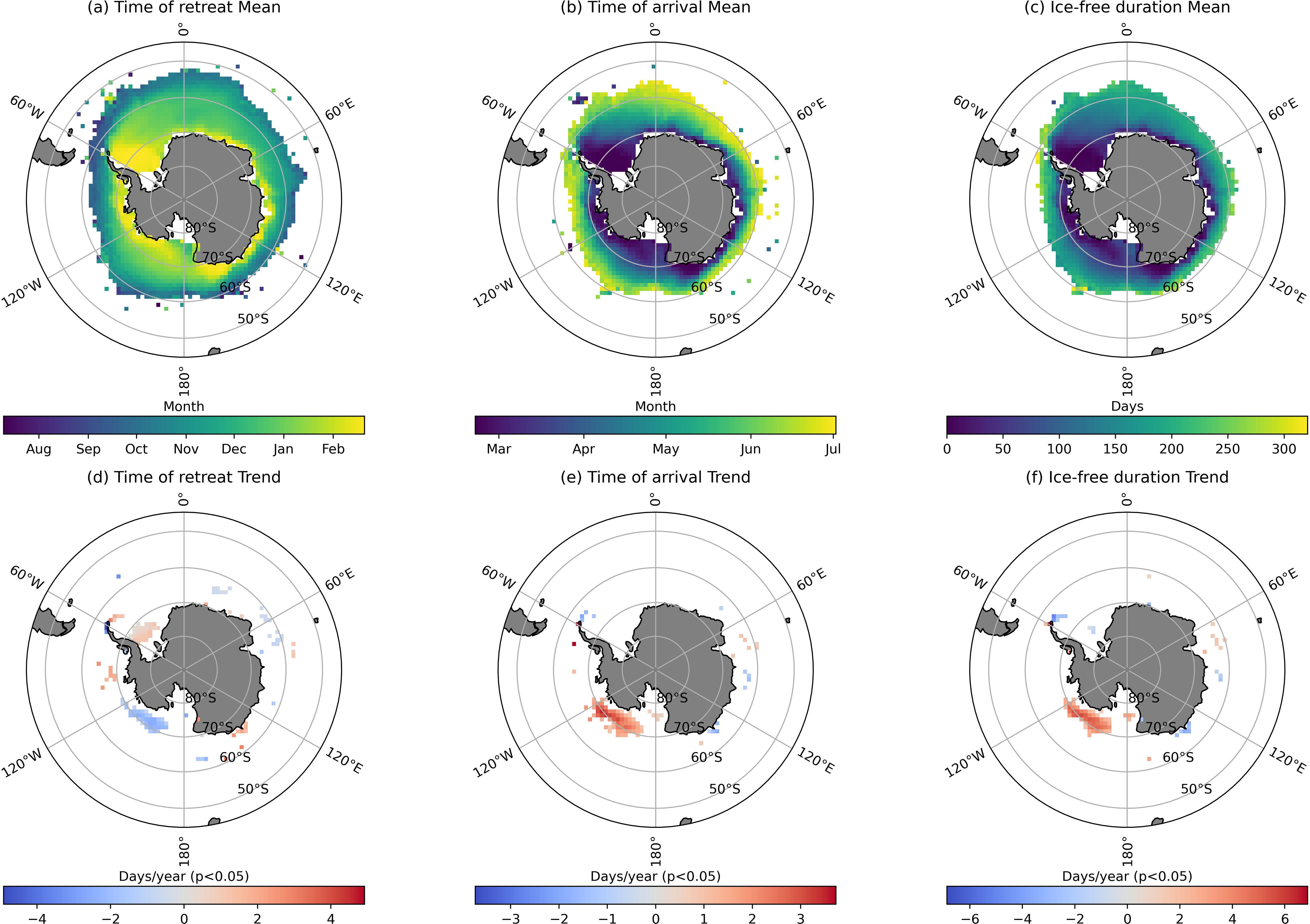
Figure 2. Mean and trend of sea ice dynamics timing parameters in 1997-2019. (A) Time of retreat annual mean. (B) Time of arrival annual mean. (C) Ice-free duration annual mean. (D) Time of retreat annual trend. (E) Time of arrival annual trend. (F) Ice-free duration annual trend.

The average sea ice formation time in the Southern Ocean from 1997 to 2019 ranged from March to July, with earlier formation near the coast and later formation in the open ocean (Figure 2B). Unlike the retreat time, sea ice formation in the Amundsen Sea showed a significant delay, with formation occurring 4 days later per year (Figure 2E). The average ice-free duration during this period indicated year-round ice coverage near the continental shelf, while regions closer to 60°S and farther north displayed ice-free conditions throughout the year (Figure 2C). Similarly, the Amundsen Sea showed a trend of increasing ice-free duration, with a maximum extension of 6 days per year (Figure 2F).

From 1997 to 2019, the average bloom initiation time in the Southern Ocean ranged from August to February of the following year, with later initiation near the coast and earlier initiation in the open ocean. In the southwestern Antarctic region, bloom initiation generally occurred around February (Figure 3A). The trend shows a significant advancement in bloom initiation at lower latitudes, with an average shift of 5 days per year (Figures 3B, C). The average bloom termination time ranged from October to May, with little spatial variation across the Southern Ocean, and was predominantly concentrated around March (Figure 3D). The bloom termination time did not exhibit a significant trend from 1997 to 2019 (Figure 3F), but in the 60°S-70°S region of the southwestern Antarctic and the D’Urville Sea, it advanced by approximately 5 days per year (Figure 3E). The average bloom duration was shorter near the coast and longer in the open ocean (Figure 3G). There was an extension in bloom duration at lower latitudes (north of 50°S), while the bloom duration near the continental shelf remained relatively unchanged (Figures 3H, I).

Figure 3

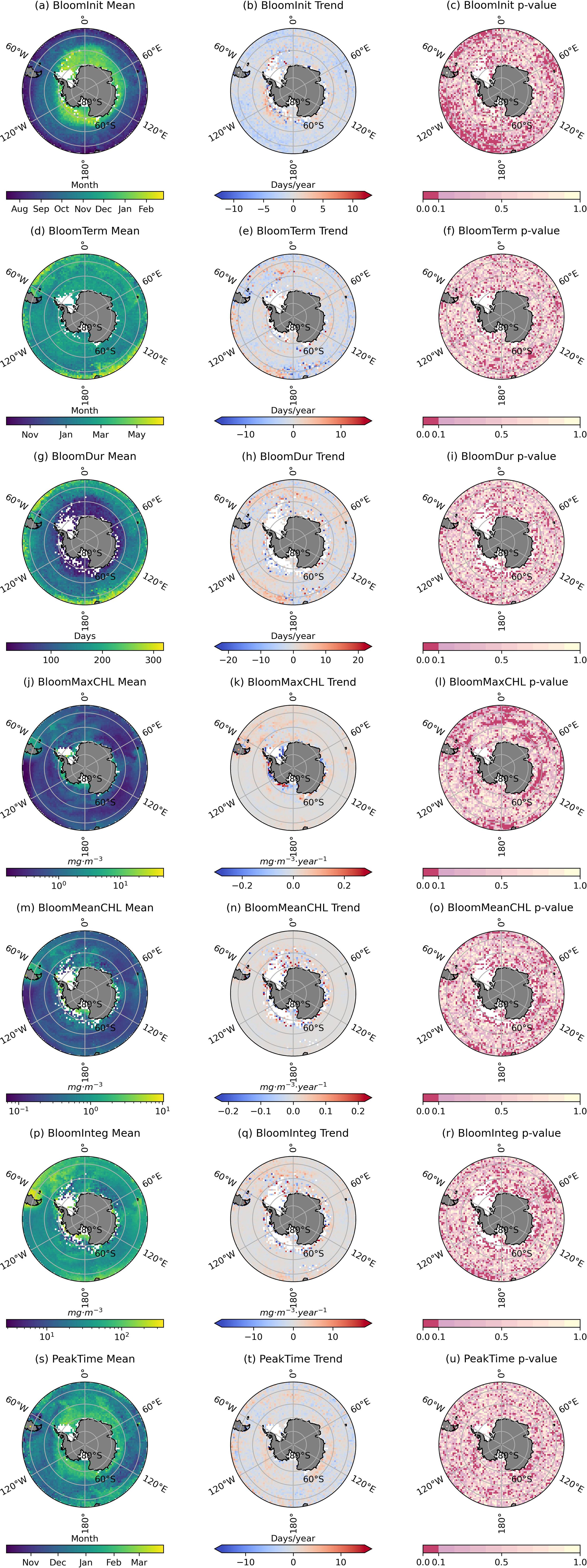
Figure 3. Mean and trend of algal bloom timing parameters in 1997-2019. (A–C) Bloom initiation date annual mean, trend, and p-value. (D–F) Bloom termination date annual mean, trend, and p-value. (G–I) Bloom duration annual mean, trend, and p-value. (J–L) Bloom maximum chlorophyll-a concentration annual mean, trend, and p-value. (M–O) Bloom mean chlorophyll-a concentration annual mean, trend, and p-value. (P–R) Bloom integrated chlorophyll-a concentration annual mean, trend, and p-value. (S–U) Bloom chlorophyll-a concentration peaking date annual mean, trend, and p-value.

During the 1997-2019 period, the peak, mean, and integrated CHL during the bloom were highest near the coast and lower in the open ocean (Figures 3J, M, P). Across the entire Southern Ocean, peak CHL during the bloom showed an upward trend, with a notable increase in the D’Urville Sea near the continental shelf, where the average CHL increased by approximately 0.05 mg·m^-3 per year (Figures 3K, L). Similarly, integrated CHL during the bloom showed a significant upward trend in the Mawson Sea (Figures 3Q, R). The peak timing of CHL during blooms in the Southern Ocean exhibits a pattern where coastal areas peak later than the open ocean. Typically, the peak date for coastal regions occurs around February (Figure 3S). At the same time, there is a notable delay in the peak timing of CHL during blooms in both the Amundsen Sea and the D'Urville Sea (Figures 3T, U).

3.1.2 Environmental factors characteristics for Antarctic krill presence

Based on the Antarctic krill presence data, matched with environmental parameters, kernel density plots were generated for four sectors (Figure 4). The results show that Antarctic krill generally appears when SST is between -2°C and 5°C. In the Ross sector, krill are concentrated in areas with SST below 0°C, with a peak at temperatures lower than 0°C. In the Lazarev sector, krill appear in both areas below 0°C and around 1°C. For the Prydz and Atlantic sectors, krill are found across a wider SST range. Specifically, in the Atlantic sector, krill are more commonly found in areas with SST above 1°C, while in the Prydz sector, krill tend to appear in areas with SST closer to 0°C (Figure 4A).

Figure 4

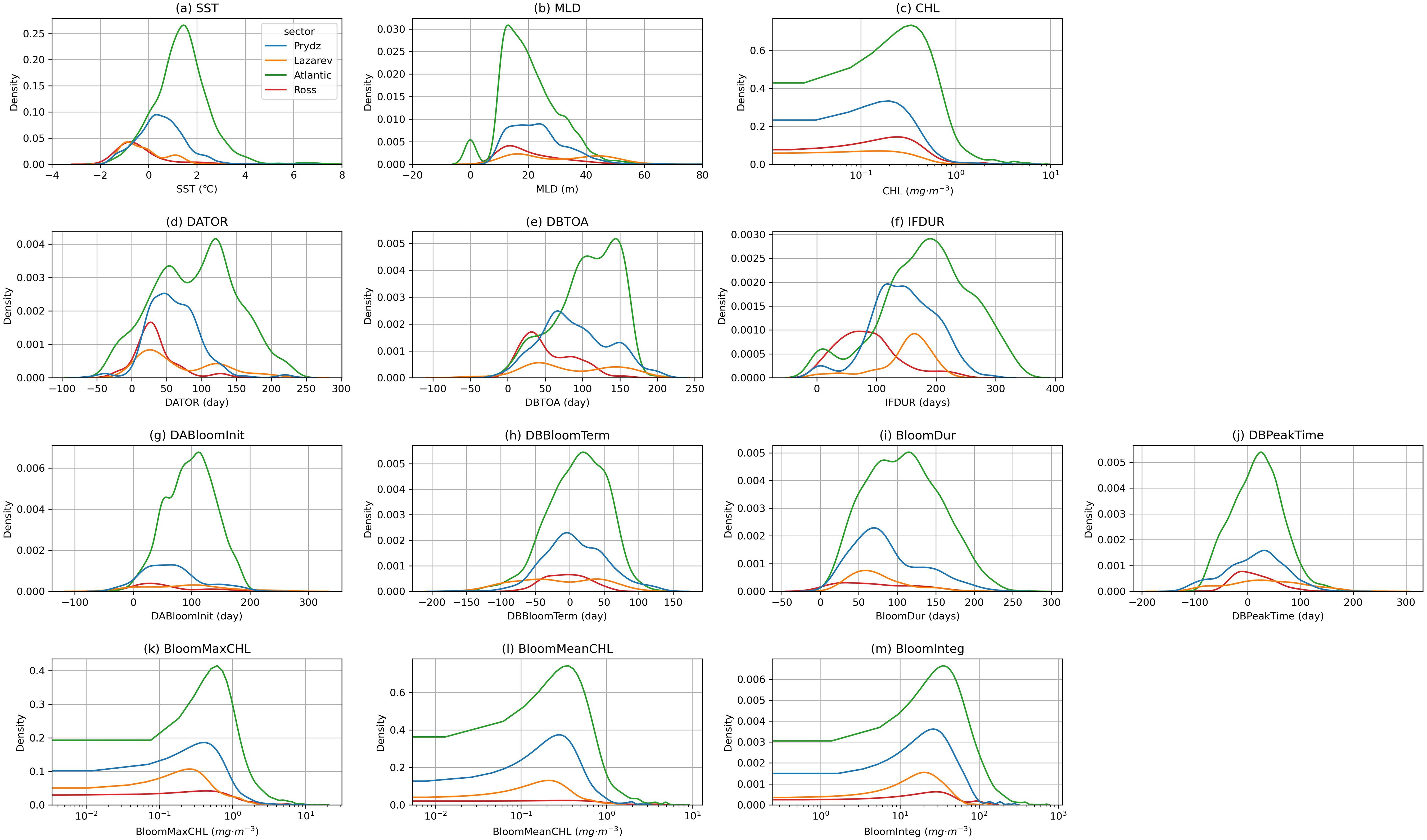
Figure 4. Kernal density estimation of krill presence matched environmental parameters: (A) SST, (B) MLD, (C) CHL, (D) DATOR, (E) DBTOA, (F) IFDUR, (G)DABloomInit, (H) DBBloomTerm, (I) BloomDur, (J) DBPeakTime, (K) BloomMaxCHL, (L) BloomMeanCHL, (M) BloomInteg.

For MLD, Antarctic krill in the Prydz sector are more frequently found in waters with an MLD less than 20 meters, while in the other three sectors, krill are predominantly found in areas where the MLD is greater than 20 meters (Figure 4B). In terms of CHL, krill in the Atlantic sector are typically found in areas with CHL around 0.3 mg·m^-3, in the Ross sector at around 0.2 mg·m^-3, and in the Prydz sector at around 0.1 mg·m^-3. The Lazarev sector does not show a distinct CHL peak (Figure 4C). It is important to note that krill surveys are usually conducted in ice-free regions, so the presence data are predominantly matched to areas with SIC near zero.

Regarding the time of sea ice retreat, Antarctic krill in the Ross and Lazarev sectors typically appear around 25 days after the sea ice has retreated, while in the Prydz sector, krill appear about 50 days after retreat. In the Atlantic sector, krill appear 50 to 120 days after sea ice retreat (Figure 4D). In relation to sea ice formation, krill in the Ross sector are observed about 30 days before ice formation, while in the Prydz sector, krill are found 60 days before formation. In the Atlantic sector, krill are observed 100 to 140 days before ice formation, while the Lazarev sector shows no clear peak (Figure 4E).

For the duration of the ice-free period, krill in the Ross sector experience the shortest duration, concentrated around 60 days. In contrast, krill in the Lazarev and Atlantic sectors experience the longest ice-free periods, around 180 days, while the Prydz sector has an ice-free period of approximately 150 days (Figure 4F).

In terms of phytoplankton bloom initiation, krill in the Atlantic sector typically appear about 100 days after bloom initiation, while in the Prydz sector, they appear around 75 days after bloom initiation. The other two sectors do not exhibit clear patterns (Figure 4G). Regarding bloom termination, krill in the Atlantic sector generally appear 20 to 50 days after bloom termination, while krill in the Prydz sector appear right as the bloom ends (Figure 4H). For bloom duration, krill in the Atlantic sector are more frequently found in areas where the bloom lasts 80 to 120 days, while in the Prydz sector, the bloom duration is around 75 days (Figure 4I). For the timing of CHL peaks during blooms, Antarctic krill in the Atlantic and Prydz sectors typically appear before the CHL peak, while in the Ross sector, they are observed after the CHL peak (Figure 4J).

When examining CHL peaks, mean values, and integrated CHL during the bloom, the results indicate the highest concentrations in the Atlantic sector, followed by the Prydz and Lazarev sectors, with the Ross sector showing no distinct peak (Figures 4K-M).

3.2 Suitability model validation and comparisons

For the original matched dataset, we tested the optimal combinations of 11–14 environmental parameters (with the minimum GCV for the same number of input parameters). Subsequently, we evaluated the optimal combination of environmental parameters by minimizing the number of non-null input factors required to predict suitability. Several model sets were constructed and compared for classification accuracy and generalization ability (Table 3). During the process of reducing the total number of input parameters to find the optimal variable combination, we observed that as the overall number of inputs decreased, the GCV continued to decline. However, when the input parameters were reduced from 12 to 11, both the AUC and TSS showed a decrease, indicating a decline in the model’s classification ability, while the GCV only improved by 0.0001. Therefore, we chose the optimal combination with 12 input parameters for further training. Compared to the original model with 14 environmental parameters, the model performance increase when the factors with strong collinearity, BloomDur, and IFDUR, were removed, leading to an decrease in GCV and increase in AUC and TSS.

Table 3

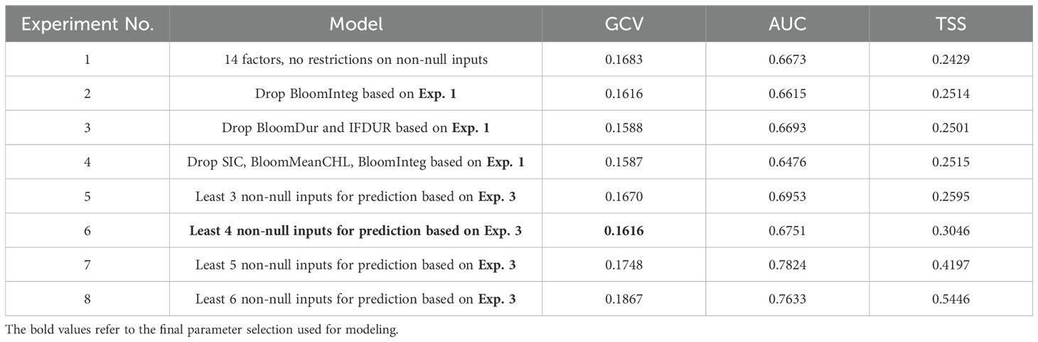
Table 3. ROC-AUC, TSS and genuine cross validation scores for each modeling experiment.

Since MLD, SIC, and SST had no missing data, we initially established a requirement of at least three non-null environmental variables for predicting suitability; otherwise, the output would be null. We gradually increased the minimum number of non-null input parameters from three to six and found that having at least four non-null values resulted in the lowest GCV (Table 3). Consequently, we set the final model to require a minimum of four non-null inputs from the optimal combination of 12 environmental parameters.

The final model, built using 12 environmental parameters, see Figure 5A for the detail inputs, which showed that the highest contributing factors were SST, TOR, BloomMaxCHL and MLD. Among them, the timing parameters of sea ice dynamics and phytoplankton bloom contributed significantly more to the model than single-time CHL and SIC values (Figure 5A). In contrast, BloomMeanCHL, BloomInteg, and SIC had the lowest contributions to the model. SIC has low effectiveness in distinguishing Antarctic krill habitats primarily because it consists mostly of zero values, particularly since most observational data were collected in areas without sea ice cover. Meanwhile, BloomMeanCHL and BloomInteg provide limited effective information due to their high collinearity with other chlorophyll parameters.

Figure 5

Figure 5. (A) Feature importance of CatBoost-based suitability model, (B) ROC curves from multiple time modeling, and (C) GCV-based model validation.

It is important to note that the optimal combinations of environmental parameters, under the constraint of a limited number of input variables, are derived from filtering all possible combinations based on the minimum GCV. Despite the AUC performing poorly according to the classification performance standards: failing (0.5–0.6), poor (0.6–0.7), fair (0.7–0.8), good (0.8–0.9), and excellent (0.9–1.0) (Phillips et al., 2006), some years could not calculate the AUC due to a single category and had a smaller MSE (Figure 5C). As a result, the actual classification accuracy should be AUC > 0.675 (Figure 5B). Overall, the model was effective in reconstructing the historical habitat suitability of Antarctic krill and could be reliably used for modeling their habitat suitability.

3.3 Predicted Antarctic krill habitat suitability

3.3.1 Highly suitable Antarctic krill habitat seasonal and annual variations

Based on the months included in the survey data and the life cycle of Antarctic krill, the habitat suitability model constructed using CatBoost was restricted to the period from November to April for reconstructing Antarctic krill habitat suitability. The monthly average habitat suitability for Antarctic krill from 1997 to 2019 was calculated (Figure 6). Habitat suitability was classified into four categories: Unsuitable (below 0.4), Marginally suitable (0.4-0.6), Moderately suitable (0.6-0.8), and Highly suitable (0.8-1.0).

Figure 6

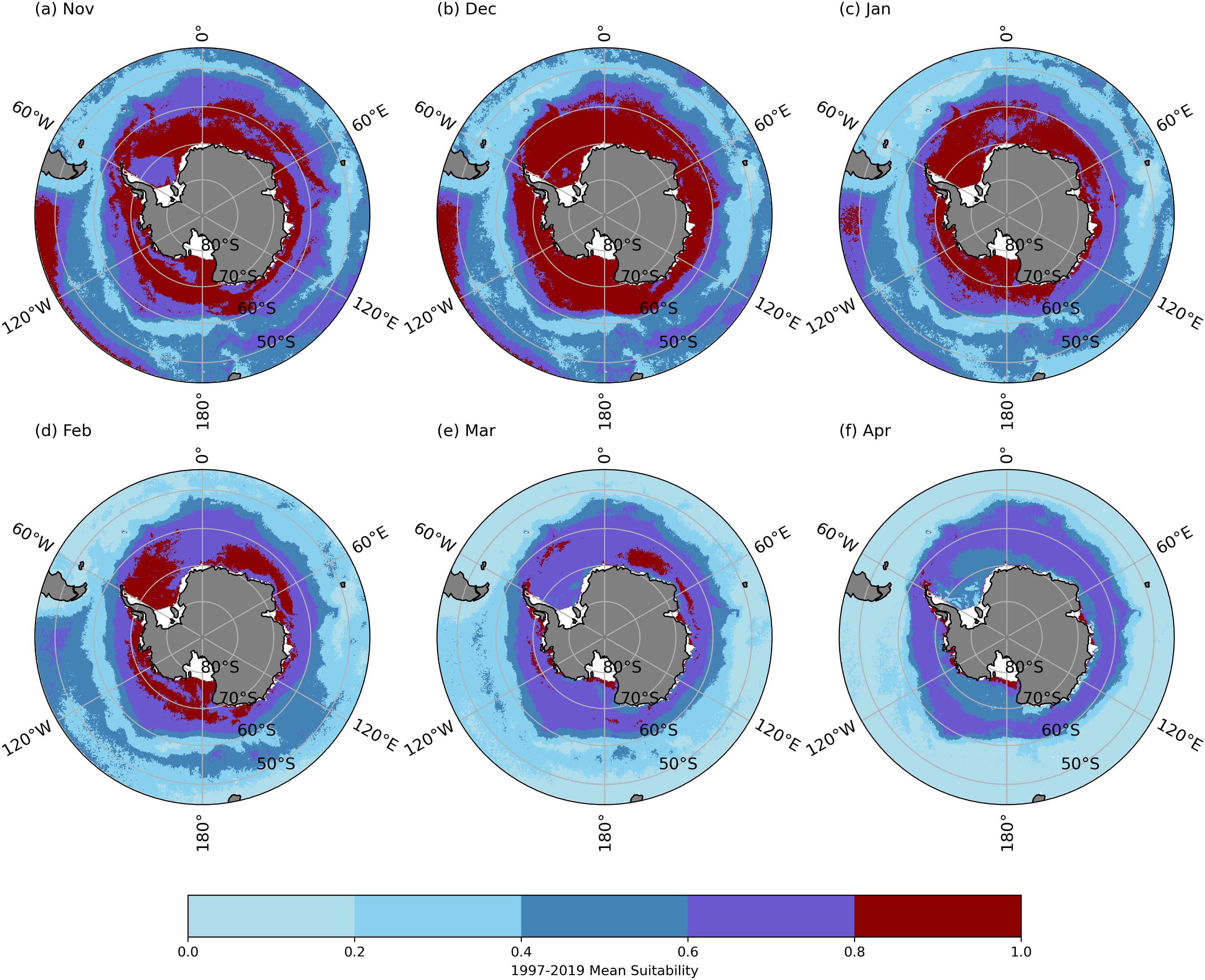
Figure 6. Monthly mean Antarctic krill habitat suitability in 1997-2019. (A) November; (B) December; (C) January; (D) February; (E) March; (F) April.

In November, the average habitat suitability for Antarctic krill in the Southern Ocean showed higher suitability near the continental shelf, lower suitability near the 60°S latitude, and higher suitability north of 60°S. By December, the region with lower suitability in the middle had increased (Figures 6A, B). From January to March, the highly suitable habitat for Antarctic krill consistently remained in the waters south of 60°S near the continental shelf, and the moderately suitable habitat between 60°W and 180°W exhibited a dynamic shift toward higher latitudes. In the D’Urville Sea, the suitability of krill habitats increased and contracted towards higher latitudes near the coast. By April, the most suitable krill habitats were concentrated around the Antarctic continental shelf (Figures 6C-F).

The highly suitable regions for Antarctic krill (Suitability > 0.8) were extracted, and the annual area of Antarctic krill habitat was calculated for the four sectors (Figure 7). Notably, the highly suitable habitat area for Antarctic krill in the Atlantic Sector reached its maximum extent in 2005 but exhibited a significant decline by 2019. Similarly, the Lazarev Sector reached its peak one year later, in 2006, followed by a noticeable reduction. In contrast, the highly suitable habitat area in the Prydz Sector demonstrated a more prolonged declining trend. Meanwhile, the Ross Sector showed a peak in its highly suitable habitat area at a time similar to that of the Atlantic and Lazarev Sectors.

Figure 7

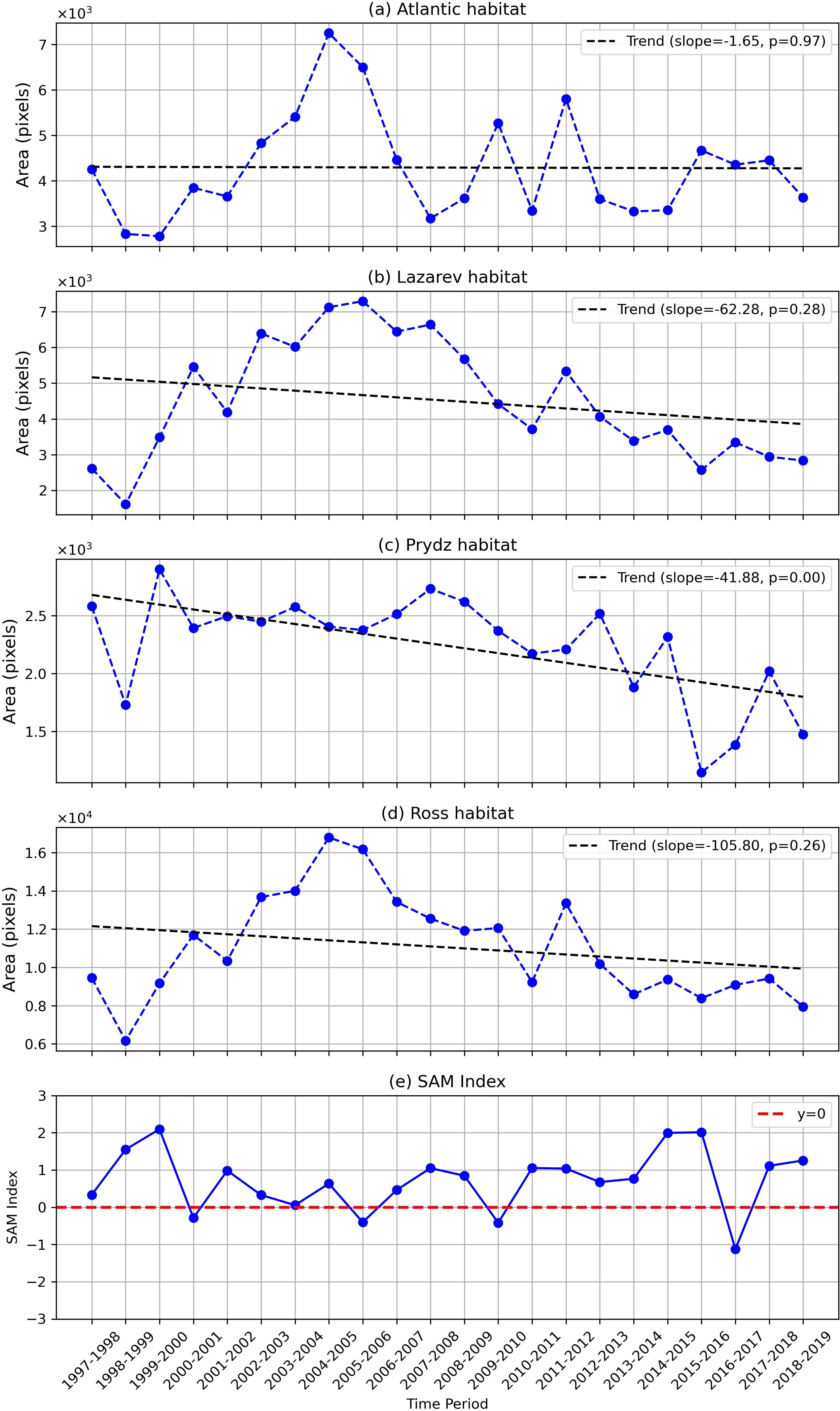
Figure 7. Antarctic krill highly suitable habitat area variation in 1997-2019 in 4 sectors: (A) Atlantic sector; (B) Lazarev sector; (C) Prydz sector; (D) Ross sector. (E) annual mean SAM index from November to April (calculated from Marshall, 2003).

SAM has remained in a positive phase after 2010 except for 2016 (Figure 7E), leading to intensified of zonal winds that enhance warm deep waters upwelling near the Antarctic coast, thereby reducing sea ice extent and supporting increased primary production (Fogt and Marshall, 2020; Greaves et al., 2020). Although the trends in the other three sectors were not significant, all four sectors displayed a pattern of initial increase followed by a decline, which corresponded with the annual trend of the SAM index. This indicates a decline in the suitability of Antarctic krill habitat that is related with the positive SAM index after 2010. It is worth noting that the area of highly suitable habitat for Antarctic krill in the Prydz sector demonstrated a significant overall declining trend from 1997 to 2019.

3.3.2 Antarctic krill habitat suitability spatio-temporal patterns

Using the habitat suitability model predicted by CatBoost, the daily habitat suitability of Antarctic krill from November to April during the period 1997-2019 was obtained. Based on the daily distribution of Antarctic krill habitat suitability, annual distributions of habitat suitability were calculated, along with the multi-year averages, variances, trends, and the significance of these trends (p-values) for the period from 1997 to 2019 (Figure 8). The distribution of habitat suitability showed higher values along the continental shelf and lower values toward lower latitudes. Notably, the habitat suitability for Antarctic krill exhibits distinct maxima in the coastal regions of the Ross Sea, Prydz Bay, Amundsen Sea, and the Western Antarctic Peninsula, while the habitat suitability in the Weddell Sea primarily indicates moderate suitability (Figure 8A). The zonal trend from the coastal regions towards lower latitudes shows a decrease in highly suitable habitat maxima, transitioning to moderately suitable habitats, followed by a gradual increase back to highly suitable habitats, before rapidly declining to marginally suitable habitats near 60°S. Moreover, the range of suitable habitat in the Southwestern Antarctic is significantly greater than that in the Southeastern Antarctic. Based on the multi-year variance of Antarctic krill habitat suitability, the differences in habitat suitability within the sea ice extent and the Antarctic Circumpolar Current (ACC) range are smaller compared to the variations observed at the ice edge (Figure 8B).

Figure 8

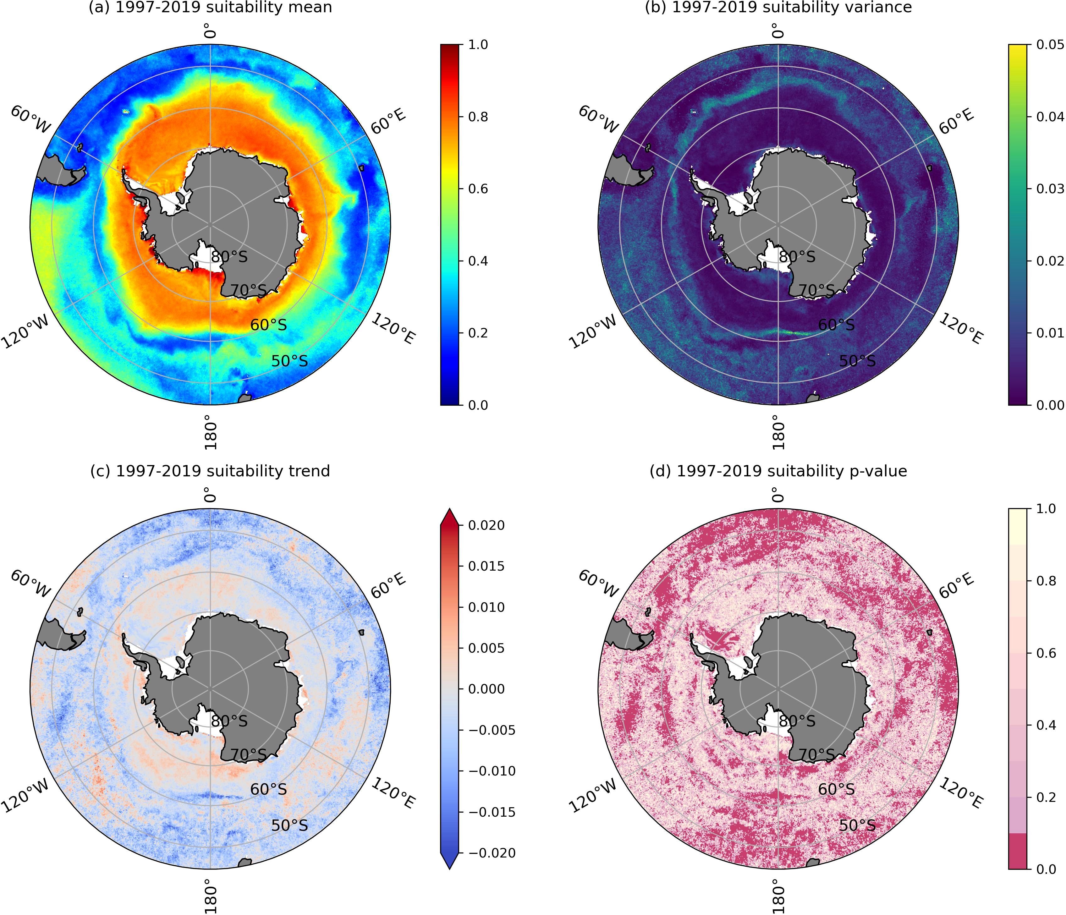
Figure 8. Mean (A), variance (B), trend (C), and p-value (D) of Antarctic krill habitat suitability from 1997 to 2019.

The trend analysis of annual mean habitat suitability for Antarctic krill from 1997 to 2019 reveals a non-significant increase in habitat suitability in the Southwestern Antarctic (Figures 8C, D). Significantly, habitat suitability has increased along the coastal region of the Western Antarctic Peninsula, Amundsen Sea, as well as in the nearshore areas of the Somov Sea. In contrast, the Weddell Sea exhibits a significant declining trend in habitat suitability. Besides, the habitat change trends in most other areas are not significant (Figure 8D).

4 Discussion

This study proposed a novel workflow for reconstructing the historical habitat suitability of Antarctic krill. Using remote sensing and reanalysis products, we calculated sea ice and phytoplankton bloom timing parameters and conducted multi-year trend analyses. Additionally, based on Antarctic krill survey data, we evaluated the habitat suitability characteristics of different regions in the Southern Ocean. For the first time, the CatBoost algorithm was applied to construct a species distribution model, offering a new approach for habitat suitability research and demonstrating the critical role of timing parameters among environmental drivers. Furthermore, we conducted a trend analysis of habitat changes over more than 20 years and identified a declining trend in Antarctic krill habitat suitability.

4.1 Impact of climate change on sea ice dynamics and phytoplankton bloom timing in the Southern Ocean

Based on the calculated sea ice parameters for 1997-2019, it was observed that the ice-free period in the Amundsen Sea has been extending (Figure 2F). Previous studies have shown that the sea ice in this region has been consistently decreasing during the Antarctic summer from 1979 to 2014 (Hobbs et al., 2016), with the timing of sea ice retreat advancing each year (Figure 4D). Although no direct cause has been identified for the earlier sea ice retreat and reduction in the Amundsen Sea, the phenomenon is closely linked to the influence of Southern Annular Mode (SAM), El Niño-Southern Oscillation (ENSO), and the Amundsen Sea low (ASL) on atmospheric circulation over the Southern Ocean (Hosking et al., 2013). Additionally, under the combined effects of ENSO and SAM, the extent of summer sea ice in the Southern Ocean is expected to increase (Pezza et al., 2012), which could explain the shortened ice-free period in the D’Urville Sea. Thus, further research of environmental factors interaction is necessary to better understand the specific physical processes and climate change effects on sea ice dynamics in different regions of the Southern Ocean in the future.

Regarding the phytoplankton bloom timing parameters from 1997 to 2019, it was found that the onset of blooms in the Southern Ocean advanced (Figure 3D), the duration of blooms lengthened (Figure 3F), and CHL during blooms increased (Figures 3J-L). These trends are consistent with the previous research, although our study only calculated bloom parameters for the Antarctic krill investigated month rather than the entire year. Nevertheless, the parameterization of phytoplankton bloom timing during this period could regulate the primary food sources (e.g. diatoms, large dinoflagellates, and other armored flagellates) availability for Antarctic krill (Flores et al., 2012a). The increase in CHL during blooms is primarily associated with rising sea surface temperatures and deeper summer mixed layers (Thomalla et al., 2023). It should be noted that although the OC-CCI products have been interpolated, there are still missing values in the coastal area due to factors like sea ice coverage. As a result, the characteristics of phytoplankton blooms in that region can’t be fully identified to provide references for predicting the distribution of Antarctic krill. Additionally, research on the Antarctic Peninsula has shown that the bloom initiation and peak dates of CHL during phytoplankton bloom in the marginal ice zone and shelf areas are delayed, which could be attributed to enhanced light limitation resulting from deeper mixing induced by increased wind speeds during spring (Turner et al., 2024). Ungapped CHL products covering the coastal areas of the Southern Ocean needs to be developed to better understand phytoplankton bloom variation.

The declining trend in SST in the Southern Ocean since 1980, attributed by many studies to SAM, contributes to Antarctic sea-ice expansion (Kostov et al., 2017; Kang et al., 2023). However, this surface cooling process in the Southern Ocean is more pronounced in the marginal ice zone in the Ross Sector (Kusahara et al., 2017; Kang et al., 2023), leading Antarctic krill in the Ross Sector stayed with lower SST. In the Lazarev Sector, while the surface cooling process in this region is not prominent, studies in the Lazarev Sea and Cosmonauts Sea have indicated that Antarctic krill in these areas are temperature-limited, tending to inhabit environments with sea temperatures below 0°C (Meyer et al., 2009; Lin et al., 2022). Simultaneously, Antarctic krill in these two sectors appear earlier following sea ice retreat compared to the other two sectors, indicating the critical role of the under-ice habitat as a primary residence and its importance in providing a colder thermal environment (Figure 4D). Antarctic krill in the Ross Sector typically inhabit areas with shorter ice-free periods (Figure 4F), despite the prolonged ice-free season in the Amundsen Sea, suggests a preference for environments with sea ice cover.

The Atlantic Sector has the most Antarctic krill survey records (Figure 1A). While fewer sampling records in the Weddell Sea due to fishing restrictions, Antarctic krill investigations in the western Antarctic Peninsula and Scotia Sea regions are abundant. Many studies indicate that the Antarctic Peninsula, a region of rapid warming influenced by atmospheric circulation and oceanic anomalies, is distinguished from other sectors of the Southern Ocean by the retreat of sea ice and rising sea surface temperatures (Li et al., 2014; Sato et al., 2021). Therefore, in the Atlantic Sector, Antarctic krill appear at higher temperature ranges (1-2°C), experience the longest ice-free period, and the warmer seawater extends the duration of phytoplankton blooms. The Prydz Sector encompasses the waters of East Antarctica, and existing studies have reflected SST warming from 1996 to 2013 through diatoms collected in sediment cores from Prydz Bay (Huang et al., 2023). The anomalous warming in this region during 2016-2017 is also noteworthy, as it is expected to have a direct impact on the Antarctic krill populations in the area (Sabu et al., 2021). Meanwhile, the ice shelf melt in the D’Urville Sea cools and freshens the subsurface ocean while warming the upper layers (Huot et al., 2021). Therefore, the suitable temperature range for Antarctic krill in the Prydz Sector is second only to that in the Atlantic Sector, and the characteristics of sea ice and phytoplankton blooms follow a similar pattern.

4.2 The impact mechanisms of environmental drivers on the Antarctic krill habitat suitability

Based on the extracted habitat suitability of Antarctic krill (Figure 8), Pearson correlation coefficients were calculated between habitat suitability and the key environmental variables identified in the CatBoost model: SST, BloomMaxCHL, TOR, and MLD. SST showed varying correlations with krill habitat suitability across regions. In coastal areas along the continental shelf, lower sea surface temperatures were associated with higher habitat suitability, while south of 60°S, higher SST correlated with higher habitat suitability. Moreover, a negative correlation between krill and SST is observed in coastal areas, while the suitability of krill south of 60°S is positively correlated with SST (Figure 9A). Krill larvae prefer stable temperatures around −1-0°C for hatching, whereas adult krill thrive in warmer waters near 1°C or higher (Thorpe et al., 2019). Thus, while rising ocean temperatures may negatively affect krill hatching, they could benefit adult krill growth. This balance explains why the warming or cooling of sea surface in different sectors of the Southern Ocean from 1997 to 2019 did not result in a significant change in the suitable habitat area for Antarctic krill (Figure 7).

Figure 9

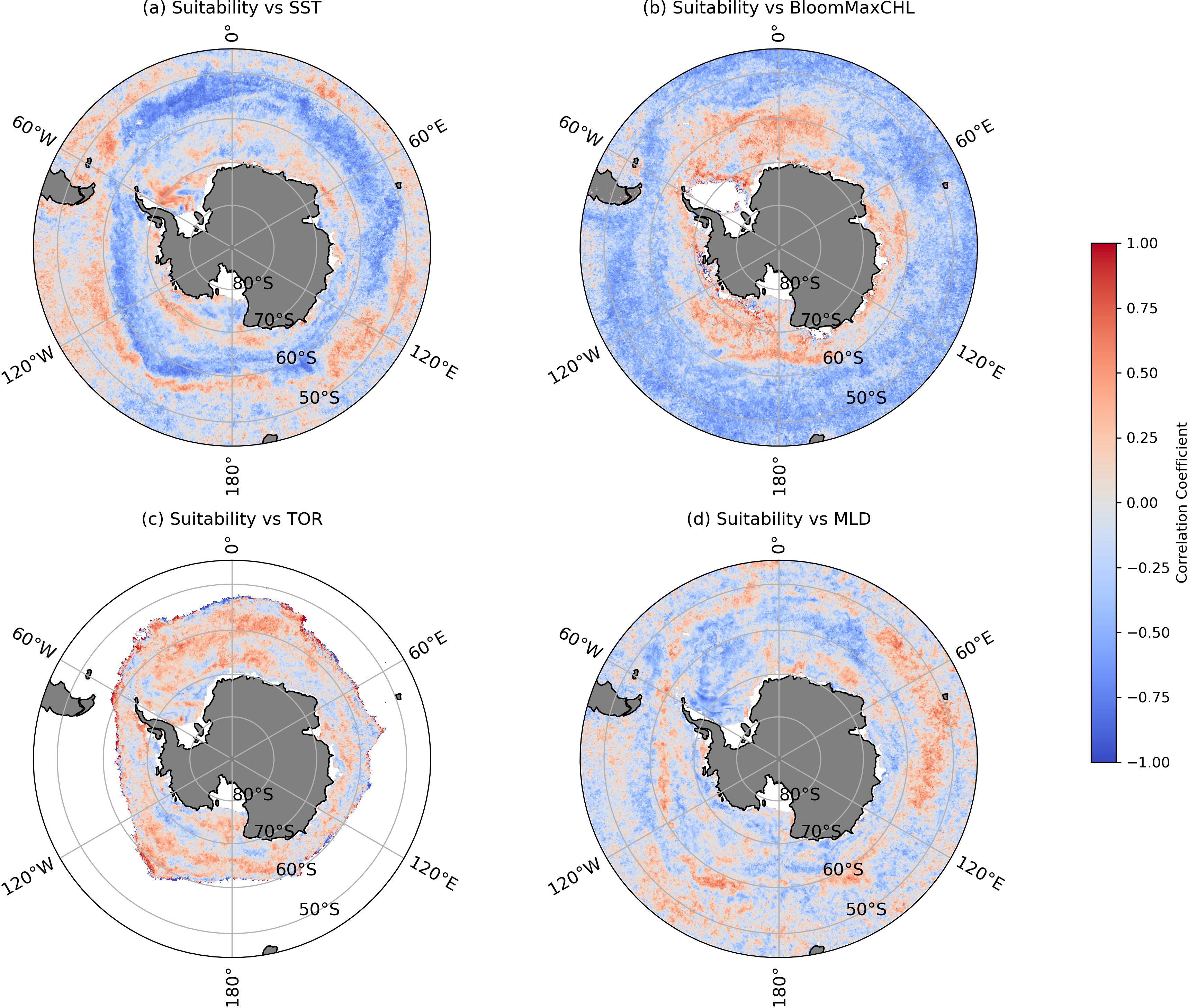
Figure 9. Key environmental factors correlation with Antarctic krill total presence days in 1997-2019: (A) SST, (B) BloomMaxCHL, (C) TOR, (D) MLD.

A positive correlation was also found between the BloomMaxCHL and krill habitat suitability south of 60°S, indicating that higher food availability supports higher habitat suitability. In contrast, in lower-latitude open ocean regions, significant negative correlations between BloomMaxCHL and krill suitability has been shown (Figure 9B). According to previous research, Antarctic krill exhibit distinct dietary structures between nearshore and open water environments: in nearshore areas, krill predominantly rely on diatoms as their primary food source, while in open waters, diatoms do not serve as the main food source for krill (Cleary et al., 2018). Although this does not rule out the possibility that Antarctic krill in open ocean environments may select diatoms as a primary food source when they are abundant, it is evident that krill gradually shift to copepods as their main food source after the postlarval growth stage (Schmidt et al., 2014). Therefore, we have reason to believe that the habitat suitability of Antarctic krill in open waters north of 60°S is less influenced by the overall abundance of phytoplankton, such as diatoms, due to their selective foraging, which is shaped by the foraging area, their growth stage, and the time of year. Seasonal variations significantly affect primary production and the accessibility of various phytoplankton groups throughout the year: when pelagic phytoplankton stocks, detected by satellite, are low, krill are more likely to seek alternative food sources such as sea ice algae, copepods, and detritus (Meyer et al., 2017).

Sea ice plays a crucial role in supporting phytoplankton reproduction, which in turn boosts krill larvae abundance in sea ice covered areas (Marrari et al., 2008). In the Weddell and Amundsen Seas, positive correlations were between sea ice retreat and habitat suitability, suggesting that later sea ice retreat corresponds to higher habitat suitability (Figure 9C). Longer durations of sea ice cover result in higher krill recruitment, as sea ice provides a source of overwintering influence and refuge for Antarctic krill larvae (Veytia et al., 2021). However, the early retreat of sea ice in the Amundsen Sea indicates a decrease in krill habitat suitability in this region. For larvae, sea ice serves as an essential food source, while it has less impact on adult krill (Walsh et al., 2020). However, the timing of sea ice retreat also determines the timing of phytoplankton blooms, making it a critical factor. The response of Antarctic krill to sea ice retreat may vary across different life stages, potentially even exhibiting opposite effects. This further highlights the differences in krill population structure between the Ross and Atlantic sectors compared to the other two sectors.

Regarding MLD, a positive correlation with krill habitat suitability was observed across most regions of the Southern Ocean, except for the Ross and Weddell Seas, where a negative correlation was found (Figure 9D). This could be caused by strong warming, leading to increased stratification and shallower MLD, which inhibits vertical mixing and limits the supply of oxygenated surface waters to deeper layers, restricting the habitat and reproductive activities of subsurface organisms (Schmidtko et al., 2017; Levin, 2018). Although studies have evaluated the relationship between MLD and krill abundance in the Ross Sea, they have not fully addressed the interannual variability of these factors (Davis et al., 2017). Furthermore, since the habitable range of MLD for Antarctic krill is often an inconsistent range in research studies, the specific biophysical processes in certain areas require further investigation.

Based on the responses of Antarctic krill habitat suitability to the 4 key variables across different regions, we can interpret the trends in Antarctic krill habitat suitability from 1997 to 2020 and their distribution characteristics in the Southern Ocean (Figure 8B). In the Atlantic Sector, the habitat suitability of Antarctic krill exhibited a growing trend in the Weddell Sea and the Antarctic Peninsula from 1997 to 2020. Although the Antarctic Peninsula is a region experiencing rapid warming, leading to a negative hatching environment for krill larvae due to rising sea temperatures, the increase in phytoplankton caused by these temperature rises has provided more food resources for Antarctic krill. In the Ross Sector, due to limitations in the Ross Sea data and the lack of a clear trend, we cannot ascertain the changes in Antarctic krill in this region. However, the suitable habitat area for Antarctic krill in this sector did experience an initial increase followed by a decrease from 1997 to 2020 (Figure 7D). In the Amundsen Sea, a region affected by climate change, despite surface cooling, the earlier retreat of sea ice has led to a decreasing trend near the continental shelf. Conversely, in the open waters at 60°S, Antarctic krill are showing an increasing trend. The reduction in sea ice provides a more prolonged growth window for phytoplankton (Arrigo et al., 2012), which can offer additional food resources for Antarctic krill in this area.

In the Lazarev Sector and Prydz Sector, the habitat suitability trend of Antarctic krill exhibits a pattern of increase, decrease, and then increase from coastal to open waters. The southeastern Antarctic region is experiencing surface cooling, which indicates an expansion of sea ice extent, a shortening of the ice-free period, and a reduction in the duration of summer phytoplankton blooms, ultimately leading to a decline in primary productivity of phytoplankton (Ludescher et al., 2019). Previous studies have documented a shift in the phytoplankton community in the Cosmonaut Sea towards smaller phytoplankton species, which may result in a transition in the zooplankton community structure from krill to salps (Li et al., 2024). Consequently, a declining trend in Antarctic krill is observed between 60°S and 70°S in the southeastern Antarctic, with a more pronounced reduction in habitat suitability for krill in the Prydz Sector since 2011 (Figure 7C). Therefore, the increasing trend of Antarctic krill habitat suitability in coastal areas and at 60°S may indicate a latitudinal migration of krill away from regions with declining phytoplankton productivity.

Overall, the impacts of climate change on the four sectors vary, resulting in different responses from Antarctic krill, making it challenging to explain these changes using a single response model. In the Atlantic Sector, warming and phytoplankton blooms have led to an increase in Antarctic krill. In the Ross Sector, the environmental dynamics of the Amundsen Sea are complex; it is influenced not only by climate factors such as the Southern Annular Mode (SAM) but is also experiencing surface cooling. Observations indicate that the timing of sea ice retreat is occurring earlier, and the ice-free period is extending, contributing to a decline in the krill population. In the Lazarev Sector and Prydz Sector, these areas follow the overall trend observed in the southeastern Antarctic, characterized by surface cooling and an increase in sea ice extent. The limited growth window for phytoplankton in these regions fails to provide adequate food resources for Antarctic krill, leading to a decrease in their population and a latitudinal migration. Although surface cooling is evident throughout the Southern Ocean, except in the Atlantic Sector, the response to sea ice varies by region; overall, however, these changes present an unfavorable trend for the Antarctic krill population.

4.3 Influence of sea ice on the Antarctic krill distribution of different life stages

The Antarctic krill survey data used in this study were not modeled to assess the habitat of Antarctic krill based on their life stages. This limitation primarily arises from the scarcity of robust data on krill life stages, as well as the challenges in achieving accuracy and consistency in the observation methods. Consequently, there was insufficient data available to train the model with the target metric requiring information such as body length. In this study, a larger amount of available survey data without specifically considering the individual life stages was collected and standardized in order to review the historical habitat suitability of Antarctic krill. Thus, the applicability of this model is subject to specific limitations. By refining relevant indices such as growth potential and recruitment index, as done in other studies (Veytia et al., 2020, 2021), and distinguishing between life stages in the model, we could further improve the capability of the model and obtain a more detailed mechanistic interpretation. Additionally, the influence of sea ice coverage on habitat selection by Antarctic krill is critical; however, the sea ice parameters used in this study are limited. More parameters, such as those related to the marginal ice zone (MIZ), need to be incorporated into the model to enhance the interpretability of sea ice effects (Veytia et al., 2021).

As mentioned earlier, the majority of surveys in this study indicate that adults constitute the primary composition of trawl survey data, compared to the larval and juvenile stages. Eggs and furcilia are likely to occur in open waters as part of their developmental ascent, whereas juveniles are typically found in coastal areas where they are sheltered by sea ice. Given the strong dependency of these life stages on under-ice habitats, the lack of sufficient under-ice survey data in this study hinders a thorough analysis of habitat suitability for juvenile Antarctic krill in nearshore regions. Thus, the inclusion of under-ice survey data is essential in Antarctic krill research. Although previous studies have investigated under-ice environments and their impact on krill distribution (Flores et al., 2012b; Meyer et al., 2017), there remains a lack of integrated long-term data and standardized research from different datasets regarding under-ice surveys. Therefore, the use of autonomous platforms capable of observing hard-to-reach areas like the under-ice environment is necessary. This approach would extend our temporal coverage of krill observations and is required to gain accurate assessments of the relationship between krill and sea ice.

4.4 The CatBoost-based suitability model for presence-absence data

This study utilized the CatBoost algorithm, based on presence-absence data, to construct a habitat suitability model for Antarctic krill and classify their habitat suitability. Previous studies have primarily used the Maxent model with presence-only data to evaluate krill habitat suitability, which led to different classification criteria (Lin et al., 2022). Although Maxent has been widely applied in species distribution modeling (SDM) for krill, it is more suited to regional-scale studies, often failing to converge when applied to larger-scale habitat reconstructions.

Many existing models and predictions for Antarctic krill are based on abundance data, such as the Krill Recruitment Index or growth potential models. However, abundance data often lacks sufficient coverage across life stages and is difficult to standardize, while occurrence data, as used in this study, provides a more comprehensive dataset for model training (Thorpe et al., 2019; Veytia et al., 2021). Most krill abundance models focus on future distribution trends under various climate scenarios, with little focus on historical habitat reconstructions. However, historical reconstructions of Antarctic krill habitat are important as they help to reveal shifts in biogeochemical cycling and predator-prey relationships (Michelson et al., 2023), constrain models of future ecological changes, enhancing predictions about the impacts of ongoing climate change (Strugnell et al., 2022), and aid in managing the expanding krill fishery, ensuring that critical spawning areas are protected (Green et al., 2021). Thus, this study aims to address this gap by offering a broader evaluation of Antarctic krill habitat suitability (Veytia et al., 2020; Lin et al., 2022; Green et al., 2023).

Nevertheless, CatBoost also has limitations in habitat suitability assessment, particularly in the classification of suitability and its relation to abundance or biomass. Further comparisons with other SDM algorithms and validation using actual sampling data are needed to refine the model. Additionally, addressing under-sampled areas in the Southern Ocean is crucial for improving the accuracy and performance of habitat suitability models for Antarctic krill.

5 Conclusion

This study integrates remote sensing and reanalysis data with Antarctic krill survey records to assess habitat suitability for Antarctic krill in the Southern Ocean. Using phytoplankton bloom and sea ice dynamics as timing parameters, a habitat suitability model was constructed using the CatBoost algorithm. For the first time, the long-term interannual variation of Antarctic krill habitat suitability over a span of more than 20 years was obtained. By combining long-term data of Antarctic environmental parameters, the study reveals the mechanisms through which environmental changes influence krill distribution and habitat suitability.

From 1997 to 2019, the ice-free period in the Amundsen Sea extended annually. Simultaneously, the onset of phytoplankton blooms advanced, their duration lengthened, and chlorophyll concentrations (CHL) during bloom periods steadily increased, particularly in coastal regions. These shifts in bloom timing and sea ice dynamics suggest that climate change is progressively impacting the Southern Ocean ecosystem. The habitat suitability of Antarctic krill is closely tied to these environmental parameters. Specifically, krill prefer areas with lower sea surface temperatures (SST), later sea ice retreat, and higher CHL during bloom periods. Krill juvenile, especially in coastal regions, are highly dependent on these conditions.

Compared to the traditional species distribution model (e.g. Maxent), CatBoost demonstrated superior ability to handle large-scale presence-absence data and provided more stable suitability predictions. The model revealed that timing parameters of bloom phenology and sea ice dynamics were more effective in explaining krill habitat suitability than conventional single-time environmental parameters. For the entire Southern Ocean, the contribution of bloom peak CHL was more indicative of krill habitat suitability than mean CHL, and sea ice retreat timing was more informative than sea ice concentration (SIC).

Model results show varying spatial and temporal trends in krill habitat suitability across different regions of the Southern Ocean between 1997 and 2019. For the four sectors, the area of high suitable habitat of Antarctic krill has shown a decline prior to Southern Annular Mode (SAM) remaining consistently positive. This trend is consistent with the positive state of SAM index. Notably, the area of highly suitable habitat for Antarctic krill in the Prydz sector has shown a significant overall decline over 20 years. The habitat suitability for Antarctic krill is generally higher in coastal areas, with a more extensive range often observed in the southwest Antarctic. In this context, the Weddell Sea has exhibited a noticeable downward trend in habitat suitability, while the Western Antarctic Peninsula has shown a significant upward trend, likely due to its status as a region experiencing rapid warming. The mechanisms of climate change effects in other sectors differ; the surface cooling that leads to increased sea ice and changes in phytoplankton communities has had varied impacts across different sectors.

In this study, we have calculated timing parameters of phytoplankton bloom and sea ice dynamic and developed a CatBoost-based suitability habitat model, reconstructing historical habitat suitability of Antarctic krill in the Southern Ocean over 20 years. The trends and patterns of phytoplankton bloom and sea ice dynamic in the Southern Ocean were identified, while also collecting characteristics on the environmental conditions associated with Antarctic krill presence. Based on predictions of historical habitat suitability, we analyze variations and trends in suitable habitat for Antarctic krill over the years, as well as their responses to climate change impacts, with a focus on four distinct sectors of the Southern Ocean. This study streamlines the standardization process of Antarctic krill survey data and employs innovative machine learning techniques to provide historical reconstruction of Antarctic krill habitat dynamics and fresh insights into the feedback mechanisms of Antarctic krill in response to climate change. By utilizing this approach, future survey data, regardless of the observational methods employed, can be integrated to reconstruct a comprehensive dataset of Antarctic krill observations in the Southern Ocean. This integration will yield a valuable overview of Antarctic krill habitats, inform fisheries management policies and protected area planning, and lay the groundwork for predicting changes in population dynamics and migrations of Antarctic krill under various climate change scenarios. Nevertheless, the application of CatBoost in species distribution modeling research can be further compared with other models to explore its suitability. In the future, under-ice Antarctic krill surveys should be widely utilized to construct a more complete dataset on the life cycle of Antarctic krill for habitat research.

Data availability statement

The original contributions presented in the study are included in the article/Supplementary Material. Further inquiries can be directed to the corresponding author.

Author contributions

YT: Conceptualization, Data curation, Formal analysis, Methodology, Software, Validation, Visualization, Writing – original draft, Writing – review & editing. YB: Conceptualization, Methodology, Writing – review & editing.

Funding

The author(s) declare financial support was received for the research, authorship, and/or publication of this article. This work was supported by the Impact and Response of Antarctic Seas to Climate Change program (grant number IRASCC2020-2022-No. 01-01-03A) and the National Naturel Science Foundation of China under Grant 42176177.

Acknowledgments

We would like to thank the Group for High-Resolution Sea Surface Temperature (GHRSST) for providing SST data (https://www.ncei.noaa.gov/data/sea-surface-temperature-optimum-interpolation), the National Snow and Ice Data Center (NSIDC) for SIC data (https://noaadata.apps.nsidc.org/NOAA/G02135/), and the European Space Agency (ESA) for Ocean Colour Climate Change Initiative (OC-CCI) products (https://www.oceancolour.org/). We also acknowledge the CMCC Global Ocean Physical Reanalysis System (C-GLORS) for providing MLD data (https://data.marine.copernicus.eu/product/) and the Global Biodiversity Information Facility (GBIF) for the Antarctic krill survey data (https://www.gbif.org/). We would also like to thank the staff of the satellite ground station, satellite data processing and sharing center, and marine satellite data online analysis platform (SatCO2) of the State Key Laboratory of Satellite Ocean Environment Dynamics, Second Institute of Oceanography, Ministry of Natural Resources of China (SOED/SIO/MNR) for their help with data processing. Finally, we sincerely thank the reviewers for their valuable comments and suggestions, which greatly improved the quality of this manuscript.

Conflict of interest

The authors declare that the research was conducted in the absence of any commercial or financial relationships that could be construed as a potential conflict of interest.

Generative AI statement

The author(s) declare that no Generative AI was used in the creation of this manuscript.

Publisher’s note

All claims expressed in this article are solely those of the authors and do not necessarily represent those of their affiliated organizations, or those of the publisher, the editors and the reviewers. Any product that may be evaluated in this article, or claim that may be made by its manufacturer, is not guaranteed or endorsed by the publisher.

Supplementary material

The Supplementary Material for this article can be found online at: https://www.frontiersin.org/articles/10.3389/fmars.2025.1513013/full#supplementary-material

References

Arrigo K. R., Lowry K. E., Van Dijken G. L. (2012). Annual changes in sea ice and phytoplankton in polynyas of the Amundsen Sea, Antarctica. Deep Sea Res. Part II: Topical Stud. Oceanography 71-76, 5–15. doi: 10.1016/j.dsr2.2012.03.006

Crossref Full Text | Google Scholar

Atkinson A., Shreeve R. S., Hirst A. G., Rothery P., Tarling G. A., Pond D. W., et al. (2006). Natural growth rates in Antarctic krill (Euphausia superba): II. Predictive models based on food, temperature, body length, sex, and maturity stage. Limnology Oceanography 51, 973–987. doi: 10.4319/lo.2006.51.2.0973

Crossref Full Text | Google Scholar

Bibik V., Maslennikov V., Pelevin A., Petrova N., Samyshev E., Soli͡Ankin E., et al. (1988). Distribution of Euphausia Superba Dana in Relation to Environmental Conditions in the Commonwealth and Cosmonaut Seas. Moscow: VNIRO Publishers.

Google Scholar

Brown M., Kawaguchi S., Candy S., Virtue P. (2010). Temperature effects on the growth and maturation of Antarctic krill (Euphausia superba). Deep Sea Res. Part II: Topical Stud. Oceanography 57, 672–682. doi: 10.1016/j.dsr2.2009.10.016

Crossref Full Text | Google Scholar

Candy S. G. (2021). Long-term trend in mean density of Antarctic krill (Euphausia superba) uncertain. Annu. Res. Rev. Biol. 36, 27–43. doi: 10.9734/arrb/2021/v36i1230460

Crossref Full Text | Google Scholar

Cavan E. L., Belcher A., Atkinson A., Hill S. L., Kawaguchi S., Mccormack S., et al. (2019). The importance of Antarctic krill in biogeochemical cycles. Nat. Commun. 10, 4742. doi: 10.1038/s41467-019-12668-7

Crossref Full Text | Google Scholar

CCAMLR (2008). Precautionary Catch Limitation on Euphausia superba in Statistical Division 58.4.2 (Hobart, Australia: CCAMLR). Available at: https://cm.ccamlr.org/en/measure-51-03-2008 (Accessed January 06, 2024).

Google Scholar

Chang W., Wang X., Yang J., Qin T. (2023). An improved catBoost-based classification model for ecological suitability of blueberries. Sensors 23 (4), 1811. doi: 10.3390/s23041811

PubMed Abstract | Crossref Full Text | Google Scholar

Cleary A. C., Durbin E. G., Casas M. C. (2018). Feeding by Antarctic krill Euphausia superba in the West Antarctic Peninsula: differences between fjords and open waters. Mar. Ecol. Prog. Ser. 595, 39–54. doi: 10.3354/meps12568

Crossref Full Text | Google Scholar

Croxall J. P., Reid K., Prince P. A. (1999). Diet, provisioning and productivity responses of marine predators to differences in availability of Antarctic krill. Mar. Ecol. Prog. Ser. 177, 115–131. doi: 10.3354/meps177115

Crossref Full Text | Google Scholar

Davis L. B., Hofmann E. E., Klinck J. M., Piñones A., Dinniman M. S. (2017). Distributions of krill and Antarctic silverfish and correlations with environmental variables in the western Ross Sea, Antarctica. Mar. Ecol. Prog. Ser. 584, 45–65. doi: 10.3354/meps12347

Crossref Full Text | Google Scholar

Ferreira A., Brito A. C., Mendes C. R. B., Brotas V., Costa R. R., Guerreiro C. V., et al. (2022). OC4-SO: A new chlorophyll-a algorithm for the western Antarctic peninsula using multi-sensor satellite data. Remote Sens. 14 (5), 1052. doi: 10.3390/rs14051052

Crossref Full Text | Google Scholar

Fetterer F., Knowles K., Meier W. N., Savoie M., Windnagel A. K. (2017). Sea Ice Index, Version 3 Sea ice concentration (Boulder, Colorado USA: National Snow and Ice Data Center).

Google Scholar

Flores H., Atkinson A., Kawaguchi S., Krafft B. A., Milinevsky G., Nicol S., et al. (2012a). Impact of climate change on Antarctic krill. Mar. Ecol. Prog. Ser. 458, 1–19. doi: 10.3354/meps09831

Crossref Full Text | Google Scholar

Flores H., Van Franeker J. A., Siegel V., Haraldsson M., Strass V., Meesters E. H., et al. (2012b). The association of Antarctic krill Euphausia superba with the under-ice habitat. PloS One 7, e31775. doi: 10.1371/journal.pone.0031775

PubMed Abstract | Crossref Full Text | Google Scholar

Fogt R. L., Marshall G. J. (2020). The Southern Annular Mode: Variability, trends, and climate impacts across the Southern Hemisphere. WIREs Climate Change 11, e652. doi: 10.1002/wcc.v11.4

Crossref Full Text | Google Scholar

Friedlaender A. S., Johnston D. W., Fraser W. R., Burns J., Patrick N H., Costa D. P. (2011). Ecological niche modeling of sympatric krill predators around Marguerite Bay, Western Antarctic Peninsula. Deep Sea Res. Part II: Topical Stud. Oceanography 58, 1729–1740. doi: 10.1016/j.dsr2.2010.11.018

Crossref Full Text | Google Scholar

Greaves B. L., Davidson A. T., Fraser A. D., Mckinlay J. P., Martin A., Mcminn A., et al. (2020). The Southern Annular Mode (SAM) influences phytoplankton communities in the seasonal ice zone of the Southern Ocean. Biogeosciences 17, 3815–3835. doi: 10.5194/bg-17-3815-2020

Crossref Full Text | Google Scholar

Green D. B., Bestley S., Corney S. P., Trebilco R., Lehodey P., Hindell M. A. (2021). Modeling Antarctic krill circumpolar spawning habitat quality to identify regions with potential to support high larval production. Geophysical Res. Lett. 48, e2020GL091206. doi: 10.1029/2020GL091206

Crossref Full Text | Google Scholar

Green D. B., Titaud O., Bestley S., Corney S. P., Hindell M. A., Trebilco R., et al. (2023). KRILLPODYM: a mechanistic, spatially resolved model of Antarctic krill distribution and abundance. Front. Mar. Sci. 10. doi: 10.3389/fmars.2023.1218003

Crossref Full Text | Google Scholar

Hancock J. T., Khoshgoftaar T. M. (2020). CatBoost for big data: an interdisciplinary review. J. Big Data 7, 94. doi: 10.1186/s40537-020-00369-8

PubMed Abstract | Crossref Full Text | Google Scholar

Hobbs W. R., Massom R., Stammerjohn S., Reid P., Williams G., Meier W. (2016). A review of recent changes in Southern Ocean sea ice, their drivers and forcings. Global Planetary Change 143, 228–250. doi: 10.1016/j.gloplacha.2016.06.008

Crossref Full Text | Google Scholar

Hosking J. S., Orr A., Marshall G. J., Turner J., Phillips T. (2013). The influence of the Amundsen–Bellingshausen seas low on the climate of west Antarctica and its representation in coupled climate model simulations. J. Climate 26, 6633–6648. doi: 10.1175/JCLI-D-12-00813.1

Crossref Full Text | Google Scholar

Huang B., Liu C., Banzon V., Freeman E., Graham G., Hankins B., et al. (2021). Improvements of the daily optimum interpolation sea surface temperature (DOISST) version 2.1. J. Climate 34, 2923–2939. doi: 10.1175/JCLI-D-20-0166.1

Crossref Full Text | Google Scholar

Huang Y., Ma R., Li J., Tu S. (2023). Sea surface temperature changes reflected by diatoms in the P6-10 core from 1893 to 2013 from Prydz bay, Antarctica. J. Mar. Sci. Eng. 11 (7), 1428. doi: 10.3390/jmse11071428

Crossref Full Text | Google Scholar

Huot P.-V., Fichefet T., Jourdain N. C., Mathiot P., Rousset C., Kittel C., et al. (2021). Influence of ocean tides and ice shelves on ocean–ice interactions and dense shelf water formation in the D’Urville Sea, Antarctica. Ocean Model. 162, 101794. doi: 10.1016/j.ocemod.2021.101794

Crossref Full Text | Google Scholar

Kang S. M., Yu Y., Deser C., Zhang X., Kang I.-S., Lee S.-S., et al. (2023). Global impacts of recent Southern Ocean cooling. Proc. Natl. Acad. Sci. 120, e2300881120. doi: 10.1073/pnas.2300881120

PubMed Abstract | Crossref Full Text | Google Scholar

Kawaguchi S., Ishida A., King R., Raymond B., Waller N., Constable A., et al. (2013). Risk maps for Antarctic krill under projected Southern Ocean acidification. Nat. Climate Change 3, 843–847. doi: 10.1038/nclimate1937

Crossref Full Text | Google Scholar

Kawaguchi S., Steven G. C., Robert K., Mikio N., Stephen N. (2006). Modelling growth of Antarctic krill. I. Growth trends with sex, length, season, and region. Mar. Ecol. Prog. Ser. 306, 1–15. doi: 10.3354/meps306001

Crossref Full Text | Google Scholar

Kohlbach D., Lange B. A., Schaafsma F. L., David C., Vortkamp M., Graeve M., et al. (2017). Ice algae-produced carbon is critical for overwintering of Antarctic krill Euphausia superba. Front. Mar. Sci. 4. doi: 10.3389/fmars.2017.00310

Crossref Full Text | Google Scholar

Kostov Y., Marshall J., Hausmann U., Armour K. C., Ferreira D., Holland M. M. (2017). Fast and slow responses of Southern Ocean sea surface temperature to SAM in coupled climate models. Climate Dynamics 48, 1595–1609. doi: 10.1007/s00382-016-3162-z

Crossref Full Text | Google Scholar

Kusahara K., Williams G. D., Massom R., Reid P., Hasumi H. (2017). Roles of wind stress and thermodynamic forcing in recent trends in Antarctic sea ice and Southern Ocean SST: An ocean-sea ice model study. Global Planetary Change 158, 103–118. doi: 10.1016/j.gloplacha.2017.09.012

Crossref Full Text | Google Scholar

Kvile K.Ø., Ashjian C., Feng Z., Zhang J., Ji R. (2018). Pushing the limit: Resilience of an Arctic copepod to environmental fluctuations. Global Change Biol. 24, 5426–5439. doi: 10.1111/gcb.2018.24.issue-11

PubMed Abstract | Crossref Full Text | Google Scholar

Levin L. A. (2018). Manifestation, drivers, and emergence of open ocean deoxygenation. Annu. Rev. Mar. Sci. 10, 229–260. doi: 10.1146/annurev-marine-121916-063359

PubMed Abstract | Crossref Full Text | Google Scholar

Li X., Holland D. M., Gerber E. P., Yoo C. (2014). Impacts of the north and tropical Atlantic Ocean on the Antarctic Peninsula and sea ice. Nature 505, 538–542. doi: 10.1038/nature12945

PubMed Abstract | Crossref Full Text | Google Scholar

Li Y., Zhao J., Li D., Pan J., He J., Hu J., et al. (2024). Factors controlling the phytoplankton crops, taxonomic composition, and particulate organic carbon stocks in the Cosmonaut Sea, East Antarctica. J. Oceanology Limnology. 42, 1859–1908. doi: 10.1007/s00343-024-3198-6

Crossref Full Text | Google Scholar

Lin S., Zhao L., Feng J. (2022). Predicted changes in the distribution of Antarctic krill in the Cosmonaut Sea under future climate change scenarios. Ecol. Indic. 142, 109234. doi: 10.1016/j.ecolind.2022.109234

Crossref Full Text | Google Scholar

Ludescher J., Yuan N., Bunde A. (2019). Detecting the statistical significance of the trends in the Antarctic sea ice extent: an indication for a turning point. Climate Dynamics 53, 237–244. doi: 10.1007/s00382-018-4579-3

Crossref Full Text | Google Scholar

Manel S., Williams H. C., Ormerod S. J. (2001). Evaluating presence–absence models in ecology: the need to account for prevalence. J. Appl. Ecol. 38, 921–931. doi: 10.1046/j.1365-2664.2001.00647.x

Crossref Full Text | Google Scholar

Marrari M., Daly K. L., Hu C. (2008). Spatial and temporal variability of SeaWiFS chlorophyll a distributions west of the Antarctic Peninsula: Implications for krill production. Deep Sea Res. Part II: Topical Stud. Oceanography 55, 377–392. doi: 10.1016/j.dsr2.2007.11.011

Crossref Full Text | Google Scholar

Marshall G. J. (2003). Trends in the Southern Annular Mode from observations and reanalyses. J. Clim. 16, 4134>–4143. doi: 10.1175/1520-0442(2003)016<4134:TITSAM>2.0.CO;2

Crossref Full Text | Google Scholar

Meyer B., Atkinson A., Bernard K. S., Brierley A. S., Driscoll R., Hill S. L., et al. (2020). Successful ecosystem-based management of Antarctic krill should address uncertainties in krill recruitment, behaviour and ecological adaptation. Commun. Earth Environ. 1, 28. doi: 10.1038/s43247-020-00026-1

Crossref Full Text | Google Scholar

Meyer B., Freier U., Grimm V., Groeneveld J., Hunt B. P. V., Kerwath S., et al. (2017). The winter pack-ice zone provides a sheltered but food-poor habitat for larval Antarctic krill. Nat. Ecol. Evol. 1, 1853–1861. doi: 10.1038/s41559-017-0368-3

PubMed Abstract | Crossref Full Text | Google Scholar

Meyer B., Fuentes V., Guerra C., Schmidt K., Atkinson A., Spahic S., et al. (2009). Physiology, growth, and development of larval krill Euphausia superba in autumn and winter in the Lazarev Sea, Antarctica. Limnology Oceanography 54, 1595–1614. doi: 10.4319/lo.2009.54.5.1595

Crossref Full Text | Google Scholar

Michelson C. I., Polito M. J., Wunder M. B., Emslie S. D., Mccarthy M. D., Patterson W. P., et al. (2023). Holocene climate change shifted Southern Ocean biogeochemical cycling and predator trophic dynamics. Limnology Oceanography 68, 2642–2653. doi: 10.1002/lno.v68.12

Crossref Full Text | Google Scholar

Murase H., Kitakado T., Hakamada T., Matsuoka K., Nishiwaki S., Naganobu M. (2013). Spatial distribution of Antarctic minke whales (Balaenoptera bonaerensis) in relation to spatial distributions of krill in the Ross Sea, Antarctica. Fisheries Oceanography 22, 154–173. doi: 10.1111/fog.2013.22.issue-3

Crossref Full Text | Google Scholar

Nachtsheim D. A., Jerosch K., Hagen W., Plötz J., Bornemann H. (2017). Habitat modelling of crabeater seals (Lobodon carcinophaga) in the Weddell Sea using the multivariate approach Maxent. Polar Biol. 40, 961–976. doi: 10.1007/s00300-016-2020-0

Crossref Full Text | Google Scholar

Pezza A. B., Rashid H. A., Simmonds I. (2012). Climate links and recent extremes in antarctic sea ice, high-latitude cyclones, Southern Annular Mode and ENSO. Climate Dynamics 38, 57–73. doi: 10.1007/s00382-011-1044-y

Crossref Full Text | Google Scholar

Phillips S. J., Anderson R. P., Schapire R. E. (2006). Maximum entropy modeling of species geographic distributions. Ecol. Model. 190, 231–259. doi: 10.1016/j.ecolmodel.2005.03.026

Crossref Full Text | Google Scholar

Piñones A., Fedorov A. V. (2016). Projected changes of Antarctic krill habitat by the end of the 21st century. Geophysical Res. Lett. 43, 8580–8589. doi: 10.1002/2016GL069656

Crossref Full Text | Google Scholar

Platt T., Fuentes-Yaco C., Frank K. T. (2003). Spring algal bloom and larval fish survival. Nature 423, 398–399. doi: 10.1038/423398b

PubMed Abstract | Crossref Full Text | Google Scholar

Prokhorenkova L., Gusev G., Vorobev A., Dorogush A. V., Gulin A. (2018). CatBoost: unbiased boosting with categorical features. Adv. Neural Inf. Process. Syst. 31, 6639–6649. doi: 10.5555/3327757.3327770

Crossref Full Text | Google Scholar

Sabu P., Subeesh M. P., Sivakrishnan K. K., Anilkumar N. (2021). Causes and impacts of anomalous warming in the Prydz Bay, East Antarctica during austral summer 2016-17. Polar Sci. 30, 100660. doi: 10.1016/j.polar.2021.100660

Crossref Full Text | Google Scholar

Sathyendranath S. J., Brockmann C., Brotas V., Calton B., Chuprin A., Clements O., et al. (2021). ESA Ocean Colour Climate Change Initiative (Ocean_Colour_cci): Version 5.0 Data. 5.0 ed (NERC EDS Centre for Environmental Data Analysis). United Kingdom: Plymouth Marine Laboratory (Science Lead), Germany: Brockmann Consult and HEREON, France: Joint Research Centre in the EU, HYGEOS, Italy: CNR, Portugal: Foundation of the Faculty of Sciences of the University of Lisbon. doi: 10.5285/1dbe7a109c0244aaad713e078fd3059a

Crossref Full Text | Google Scholar

Sato K., Inoue J., Simmonds I., Rudeva I. (2021). Antarctic Peninsula warm winters influenced by Tasman Sea temperatures. Nat. Commun. 12, 1497. doi: 10.1038/s41467-021-21773-5

PubMed Abstract | Crossref Full Text | Google Scholar

Schmidt K., Atkinson A., Pond D. W., Ireland L. C. (2014). Feeding and overwintering of Antarctic krill across its major habitats: The role of sea ice cover, water depth, and phytoplankton abundance. Limnology Oceanography 59, 17–36. doi: 10.4319/lo.2014.59.1.0017

Crossref Full Text | Google Scholar

Schmidtko S., Stramma L., Visbeck M. (2017). Decline in global oceanic oxygen content during the past five decades. Nature 542, 335–339. doi: 10.1038/nature21399

PubMed Abstract | Crossref Full Text | Google Scholar

Siegel V. (2016). “Introducing Antarctic krill Euphausia superba Dan,” in Biology and Ecology of Antarctic Krill (Springer International Publishing, Cham), 1–19.

Google Scholar

Siegel D. A., Doney S. C., Yoder J. A. (2002). The north Atlantic spring phytoplankton bloom and Sverdrup’s critical depth hypothesis. Science 296, 730–733. doi: 10.1126/science.1069174

PubMed Abstract | Crossref Full Text | Google Scholar

Stammerjohn S. E., Martinson D. G., Smith R. C., Yuan X., Rind D. (2008). Trends in Antarctic annual sea ice retreat and advance and their relation to El Niño–Southern Oscillation and Southern Annular Mode variability. J. Geophysical Research: Oceans 113, C03S90. doi: 10.1029/2007JC004269

Crossref Full Text | Google Scholar

Storto A., Masina S. (2016). C-GLORSv5: an improved multipurpose global ocean eddy-permitting physical reanalysis. Earth Syst. Sci. Data 8, 679–696. doi: 10.5194/essd-8-679-2016

Crossref Full Text | Google Scholar

Strugnell J. M., Mcgregor H. V., Wilson N. G., Meredith K. T., Chown S. L., Lau S. C. Y., et al. (2022). Emerging biological archives can reveal ecological and climatic change in Antarctica. Global Change Biol. 28, 6483–6508. doi: 10.1111/gcb.v28.22

PubMed Abstract | Crossref Full Text | Google Scholar

Taylor A. T., Hafen T., Holley C. T., González A., Long J. M. (2020). Spatial sampling bias and model complexity in stream-based species distribution models: A case study of Paddlefish (Polyodon spathula) in the Arkansas River basin, USA. Ecol. Evol. 10, 705–717. doi: 10.1002/ece3.v10.2

PubMed Abstract | Crossref Full Text | Google Scholar

Thomalla S. J., Nicholson S.-A., Ryan-Keogh T. J., Smith M. E. (2023). Widespread changes in Southern Ocean phytoplankton blooms linked to climate drivers. Nat. Climate Change 13, 975–984. doi: 10.1038/s41558-023-01768-4

Crossref Full Text | Google Scholar

Thorpe S. E., Tarling G. A., Murphy E. J. (2019). Circumpolar patterns in Antarctic krill larval recruitment: an environmentally driven model. Mar. Ecol. Prog. Ser. 613, 77–96. doi: 10.3354/meps12887

Crossref Full Text | Google Scholar

Trathan P. N., Brierley A. S., Brandon M. A., Bone D. G., Goss C., Grant S. A., et al. (2003). Oceanographic variability and changes in Antarctic krill (Euphausia superba) abundance at South Georgia. Fisheries Oceanography 12, 569–583. doi: 10.1046/j.1365-2419.2003.00268.x

Crossref Full Text | Google Scholar

Trathan P. N., Fielding S., Warwick-Evans V., Freer J., Perry F. (2022). Seabird and seal responses to the physical environment and to spatio-temporal variation in the distribution and abundance of Antarctic krill at South Georgia, with implications for local fisheries management. ICES J. Mar. Sci. 79, 2373–2388. doi: 10.1093/icesjms/fsac168

Crossref Full Text | Google Scholar

Trathan P. N., Hill S. L. (2016). “The importance of krill predation in the Southern Ocean,” in Biology and Ecology of Antarctic Krill. Ed. Siegel V. (Springer International Publishing, Cham), 321–350.

Google Scholar

Turner J. S., Dierssen H., Schofield O., Kim H. H., Stammerjohn S., Munro D. R., et al. (2024). Changing phytoplankton phenology in the marginal ice zone west of the Antarctic Peninsula. Mar. Ecol. Prog. Ser. 734, 1–21. doi: 10.3354/meps14567

Crossref Full Text | Google Scholar

Veytia D., Bestley S., Kawaguchi S., Meiners K. M., Murphy E. J., Fraser A. D., et al. (2021). Overwinter sea-ice characteristics important for Antarctic krill recruitment in the southwest Atlantic. Ecol. Indic. 129, 107934. doi: 10.1016/j.ecolind.2021.107934

Crossref Full Text | Google Scholar

Veytia D., Corney S., Meiners K. M., Kawaguchi S., Murphy E. J., Bestley S. (2020). Circumpolar projections of Antarctic krill growth potential. Nat. Climate Change 10, 568–575. doi: 10.1038/s41558-020-0758-4

Crossref Full Text | Google Scholar

Walsh J., Reiss C. S., Watters G. M. (2020). Flexibility in Antarctic krill Euphausia superba decouples diet and recruitment from overwinter sea-ice conditions in the northern Antarctic Peninsula. Mar. Ecol. Prog. Ser. 642, 1–19. doi: 10.3354/meps13325

Crossref Full Text | Google Scholar

Yang G., Atkinson A., Hill S. L., Guglielmo L., Granata A., Li C. (2021). Changing circumpolar distributions and isoscapes of Antarctic krill: Indo-Pacific habitat refuges counter long-term degradation of the Atlantic sector. Limnology Oceanography 66, 272–287. doi: 10.1002/lno.11603

Crossref Full Text | Google Scholar