Enhancing water depth inversion accuracy via SAR and variable window sliding segmentation

The utilization of synthetic aperture radar (SAR) for depth inversion is crucial for accurate underwater mapping. However, current SAR-based techniques face challenges in segmentation accuracy, which directly affects inversion precision and spatial resolution. Traditional segmentation methods lack efficiency and often result in low-resolution outcomes. To address these issues, we propose a novel SAR water depth inversion method based on variable window sliding segmentation. This method optimizes nearshore image utilization by dynamically adjusting the pixel size and preventing coastline encroachment, leading to more precise swell wavelength measurements. When applied to the eastern sea off Naraha, Japan, our method achieved a minimum mean relative error (MRE) of 9.2% for shallow waters (0 to 20 m depth) and 4.9% for deeper waters (80 to 100 m depth). These results significantly improve upon those of traditional methods, which typically show MREs ranging from 10% to 30%. Additionally, our method achieves a maximum spatial resolution of 5.5 m, a notable advancement in nearshore depth measurement. The study also revealed that different depth ranges and function types, particularly linear and atanh functions, impact measurement performance, demonstrating superior accuracy across multiple metrics.

1 Introduction

Depth inversion is a crucial area of research in marine geology and ocean resource development. With the continuous advancement of marine science and technology and the increasing demand for applications, depth inversion technology has become key in fields such as marine mapping, ocean resource exploration, and environmental monitoring. Synthetic aperture radar (SAR) technology, as a remote sensing tool, has demonstrated unique advantages and broad application prospects in depth inversioncit (Loor and Hulten, 1978; Loor, 1981; McLeish et al., 1981; Valenzuela et al., 1983).

Traditional depth measurement methods mainly include lead-line sounding and sonar sounding (Wu et al., 2013). Lead-line sounding, which measures depth by lowering a weighted line to the seabed, is a simple but inefficient method suitable for local shallow water measurements. Sonar sounding, which uses sound wave propagation characteristics, can be divided into single-beam sonar and multibeam sonar (Yang et al., 2023; Qi et al., 2023). Single-beam sonar has limited coverage and lower efficiency, whereas multibeam sonar offers broader and more accurate measurements but is expensive and complex to operate. Additionally, side-scan sonar, which is primarily used for seabed topography mapping, can also assist in depth measurement.

With the development of remote sensing technology, depth inversion methods have garnered increasing attention. Optical remote sensing, which analyzes multispectral images acquired by satellites or aircraft and combines empirical models to estimate depth, is suitable for clear, shallow waters but is affected by water transparency and suspended particles (Jay and Guillaume, 2016). Airborne light detection and ranging (LiDAR) bathymetry, which uses laser pulses to measure depth, is suitable for high-precision measurements in shallow waters and coastlines but is limited by depth, high costs and operational complexity (Wang et al., 2022). Despite the achievements of these methods, their limitations are apparent.

As SAR technology evolves and has broader applications (Mao et al., 2022; Zhou et al., 2023; Zhang et al., 2024a, b; Cao et al., 2024), the use of SAR data for depth inversion has emerged as a new, effective method (Alpers and Hennings, 1984; Zheng et al., 2006). SAR technology, through the transmission and reception of microwave signals, can acquire surface reflection signals without being constrained by weather, time, and light conditions, thereby obtaining sea surface characteristic information (Mao et al., 2021). Compared with optical remote sensing, SAR technology offers all-weather, all-time observation capabilities, making it particularly suitable for ocean regions with poor atmospheric transparency or severe cloud cover. Thus, using SAR technology for depth inversion overcomes the natural condition limitations of traditional methods, enabling efficient and accurate ocean depth detection.

In depth inversion study, SAR technology derives depth information mainly by analyzing sea surface reflection signals. Given the relationships between depth and factors such as ocean surface waves and tides, analyzing wave characteristics and reflection intensity in SAR images can reveal depth distribution patterns (Zheng et al., 2012; Li et al., 2009). Traditional inversion methods are based on complex physical equations and radar backscatter models and achieve shallow sea topography inversion by directly solving the SAR imaging process (Alpers and Hennings, 1984; Shuchman et al., 1985). This approach performs well in areas with continuous seabed terrain variations but requires high-quality SAR images. The complexity of the marine environment and the impact of SAR image noise limit the practical application of this method (Huang et al., 2000). Methods based on strong tidal currents and local seabed interactions, while theoretically innovative, face challenges such as computational complexity, sensitivity to initial depth accuracy, and relatively low detection resolution.

Therefore, continuous exploration of new techniques and methods is necessary to improve inversion accuracy and reliability in shallow sea topography. Currently, a method that relies on the refraction and shoaling of long surface gravity waves propagating toward the coast, establishing a direct relationship between swell and depth, is gradually being applied for depth inversion (Boccia et al., 2015; Bian et al., 2020; Brusch et al., 2011). With the advancement of spaceborne SAR technology, more SAR satellite data are being used for shallow sea topography detection. Using the fast Fourier transform to calculate wave information and combining it with the linear dispersion relation for depth inversion has yielded good results (Pleskachevsky et al., 2011; Misra et al., 2020). Satellites such as ERS-2, RESAT-1, HJ-1C SAR, and Sentinel-2 have been applied in depth detection experiments, demonstrating the feasibility of depth detection on the basis of swell characteristics and linear dispersion relationships (Fan et al., 2008; Mishra et al., 2014; Bian et al., 2016; de Michele et al., 2021).

The use of the linear dispersion relation to obtain water depth from SAR data has significantly enhanced the precision and efficiency of depth inversion, offering a powerful tool for mapping seabed topography. However, this method still faces several challenges that need to be addressed to improve its accuracy, especially in regions with uneven or complex seabed terrain. One of the primary challenges lies in the accurate extraction of wave wavelength information, which is central to depth inversion via the linear dispersion relation. The size and segmentation of image units are crucial factors in this wavelength extraction process. Previous studies have often relied on fixed image unit sizes ranging from 5 to 10 times the wavelength (Huang et al., 2021). While this approach may work in relatively stable environments, it becomes problematic when the wavelength varies with depth erratically. Applying a constant image unit size across the entire remote sensing image assumes that the wavelength varies uniformly, which is rarely the case, particularly in areas with significant variations in water depth. This leads to decreased accuracy and efficiency, as wavelength information may be distorted or inaccurately captured. Furthermore, human activities and irregular coastlines introduce additional complexities in nearshore areas. Coastal development, such as ports, breakwaters, and underwater infrastructure, can significantly alter wave patterns and complicate the segmentation process. Irregular coastal terrains, combined with rapidly changing seabed features, make applying a fixed image unit size difficult, further reducing the method’s reliability in regions with dynamic or complex coastal changes. To overcome these challenges, more adaptive and sophisticated algorithms are required to dynamically adjust image unit size and segmentation parameters to accommodate the local variations in wavelength and depth.

To address these issues, we propose a depth inversion method based on variable window image unit segmentation. This method dynamically adjusts the size of image units during segmentation, determines unit changes via linear functions, atanh functions, and their symmetric functions to accurately extract wavelength information in different areas, avoiding complex manual judgments and enhancing segmentation efficiency and inversion accuracy. For irregular coastlines, this method increases the utilization rate of image depth inversion in nearshore areas by transforming the starting point along the coastline and extending outward. We applied and tested this method in the sea area east of Naraha, Japan, with satisfactory results.

2 Materials and methods

2.1 Study area and materials

The eastern coast of Japan, situated in the northwestern Pacific Ocean, is closely connected to the broader Pacific Ocean. This coastal region exhibits significant variability in water depth and presents complex topographical features. The relatively shallow coastal waters provide a rich habitat for marine life, making this area one of Japan’s essential fishing centers. Geologically, the eastern coast lies at the boundary between the Pacific Plate and the Philippine Sea Plate, resulting in frequent geological activities such as earthquakes and volcanic eruptions. Additionally, coastlines are highly irregular, forming numerous excellent harbors and ports that facilitate marine trade and transportation.

As shown in Figure 1, The study area selected for this research is the waters near Naraha, a city in Fukushima Prefecture, Japan, located along the eastern coast. Naraha’s coastline stretches approximately 50 km and is characterized by its winding and variable nature, with complex topography. The surrounding mountains and hilly terrain cause the coastline to be sinuous and undulating, creating many natural bays and ports. Owing to its location in a seismic zone, frequent geological activity may lead to changes in the coastline. Additionally, influenced by the Pacific climate, the coastline may experience variations due to monsoons and oceanic fluctuations, affecting coastal topography.

Figure 1

Figure 1. Study area. The dashed box represents the depth inversion area in this study.

The Gaofen-3 (GF-3) satellite is a high-resolution radar satellite from China that was successfully launched on August 10, 2016, at the Taiyuan Satellite Launch Center. The GF-3 satellite boasts 12 imaging modes, making it the satellite with the most imaging modes among SAR satellites globally (Liang et al., 2024). In depth inversion, the GF-3 satellite has exceptional technical advantages. First, it offers a spatial resolution of up to 1 meter, enabling the satellite to precisely capture minute details of the sea surface, providing fine-grained data crucial for depth inversion. Additionally, the application of multipolarization SAR technology allows the satellite to obtain more comprehensive sea surface scattering information. These parameters are essential for improving the accuracy and reliability of depth inversion.

In this study, we utilized the Fine Stripmap 1 mode of the GF-3 satellite, which achieves a resolution of 5 m and a swath width of 50 km, with dual-polarization capabilities. Compared with other satellites, GF-3 has a strong ability to observe sea surface fluctuations. As shown in Figure 2, the entire remote sensing image was extracted to analyze surface wave patterns across different coastal regions. Subfigures 2(B) to 2(E) display areas within the red dashed box, progressively moving farther from the coastline, with each subfigure highlighting the swell characteristics at varying distances from the shore. Specifically, Figure 2B illustrates the region closest to the coast, where the swell is most prominent, exhibiting strong and well-defined patterns typical of the nearshore environment. Figure 2C captures a slightly offshore area where the swell patterns remain visible, albeit with reduced intensity as the distance from the shore increases. Figure 2D shows a more distant offshore region, where the swell is still detectable, though it appears less pronounced and more dispersed, indicating the influence of deeper waters. Finally, Figure 2E depicts the furthest offshore area, where the swell is subtle but still discernible, demonstrating the persistence of wave propagation over large distances from the coastline. The variations in pattern across these different distances are crucial for depth inversion, as they provide valuable insights into wave dynamics, which are essential for understanding depth features.

Figure 2

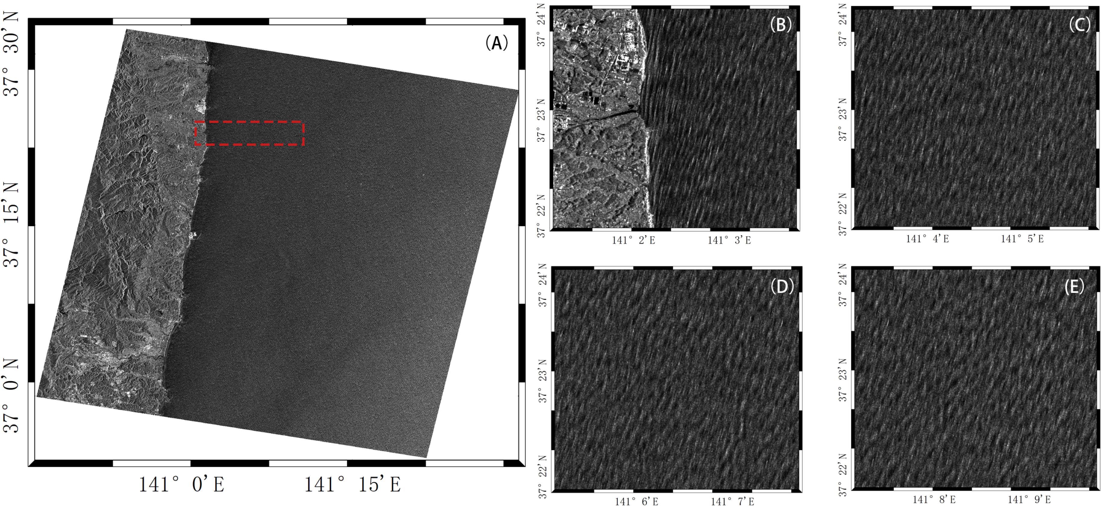
Figure 2. High-resolution SAR remote sensing image from the GF-3 satellite, acquired on March 8, 2018. (B–E) depict images gradually moving away from the coastline outlined in (A).

2.2 Image segmentation method

To perform depth inversion, a single remote sensing image needs to be segmented into multiple small image elements, each processed individually to determine the corresponding water depth. However, given that the variation in water depth is relatively small compared with the wide range of remote sensing images, manual selection of image elements during segmentation can reduce the inversion efficiency. Therefore, choosing image elements is fundamental to depth inversion and crucial for accuracy.

Previous studies have examined the influence of image elements on depth inversion and suggested appropriate ranges for these elements. However, as the observation capabilities of different remote sensing images vary, finer adjustments to the image elements are needed. Considering that the wavelength of surface waves is positively correlated with shallow water depth, the image elements should also vary during segmentation. Traditional segmentation methods are usually fixed or manually determined, significantly reducing efficiency. Such ambiguous segmentation methods often hinder reproducibility when wave information is used for depth inversion. Therefore, this study proposes a variable window sliding segmentation method for image segmentation. As illustrated in Figure 3, the process is as follows:

Figure 3

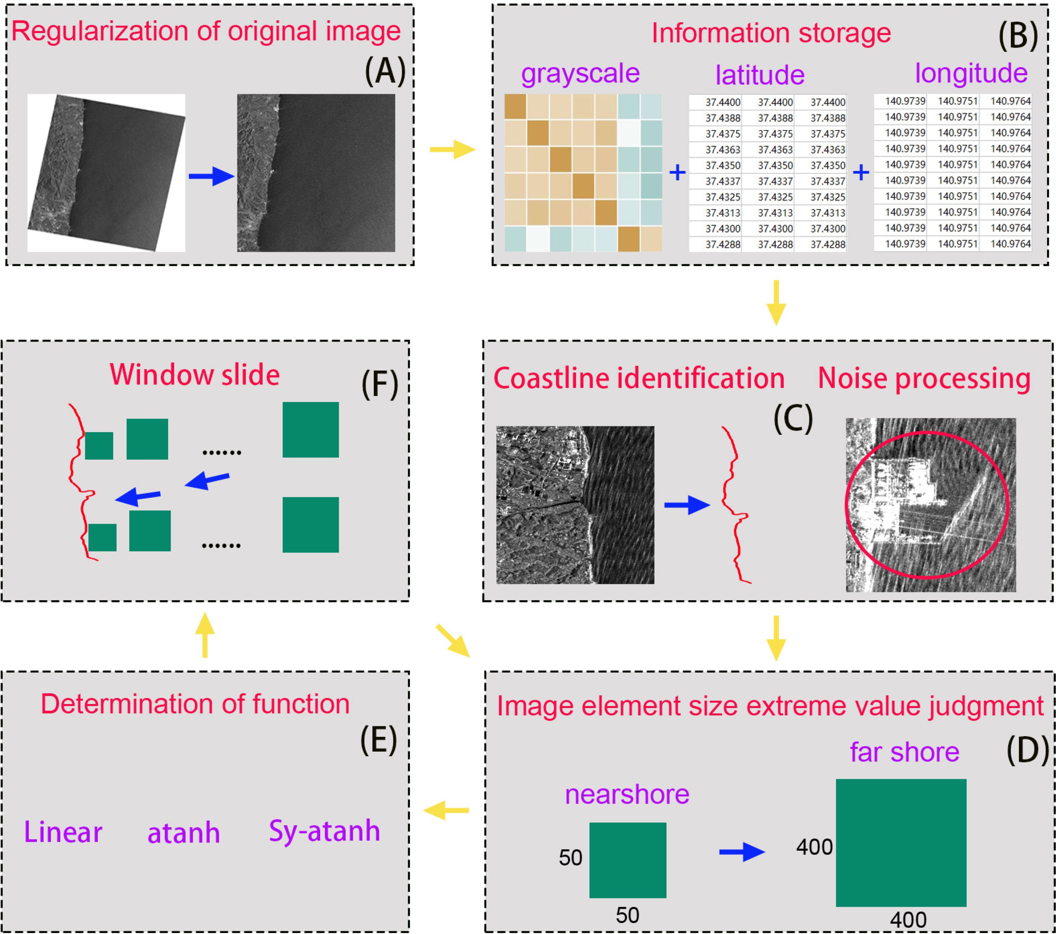
Figure 3. Process of the remote sensing image segmentation method. (A–E) correspond to each step in the method, including regularization of original image, information storage, coastline identification and noise processing, image element size extreme value judgment, determination of function, and window slide.

2.2.1 Image preprocessing

The irregular remote sensing image is adjusted to obtain a regular image, as shown in Figure 3A. The original image is not a regular rectangle, leading to some null values at the edges during segmentation. These null values introduce errors into the image unit spectrum. The adjustment aims to eliminate the influence of edge null values, thereby improving the depth inversion accuracy at the image edges.

2.2.2 Information storage

A remote sensing image is stored as an intensity information matrix and a position information matrix via software. Separating the two types of data ensures that only the intensity information matrix is manipulated during sliding window image segmentation. This separation also makes it easier to retrieve corresponding latitude and longitude information for the varying image units, thereby enhancing segmentation efficiency.

2.2.3 Coastline identification and noise processing

Software or programs are used to identify coastlines and coastal obstacles, such as ports and ships, in remote sensing images, avoiding the introduction of external interference. The impact of the coastline and external interference on the spectrum is mainly observed in shallow water areas because the image units are smaller in these areas, making the influence of the coastline and noise more noticeable. Thus, it is necessary to determine the coastline shape before image unit segmentation to provide a starting point for subsequent segmentation. Ships, oil slicks, internal waves, and other factors are considered noise when extracting wave length information of surface waves, and these areas are typically masked during the processing stage to prevent them from interfering with the analysis. Noise is reduced by averaging surrounding pixels, thus minimizing inversion errors.

2.2.4 Image unit extremum determination

The dynamic adjustment of image units requires a clear range. An appropriate segmentation range allows for more accurate retrieval of wavelength distribution information. A rough range can be obtained through simple trials. In this study, as shown in Figure 4, the image unit size increases gradually from the coastline to the open sea, with the smallest unit being 50×50 pixels and the largest being 400×400 pixels.

Figure 4

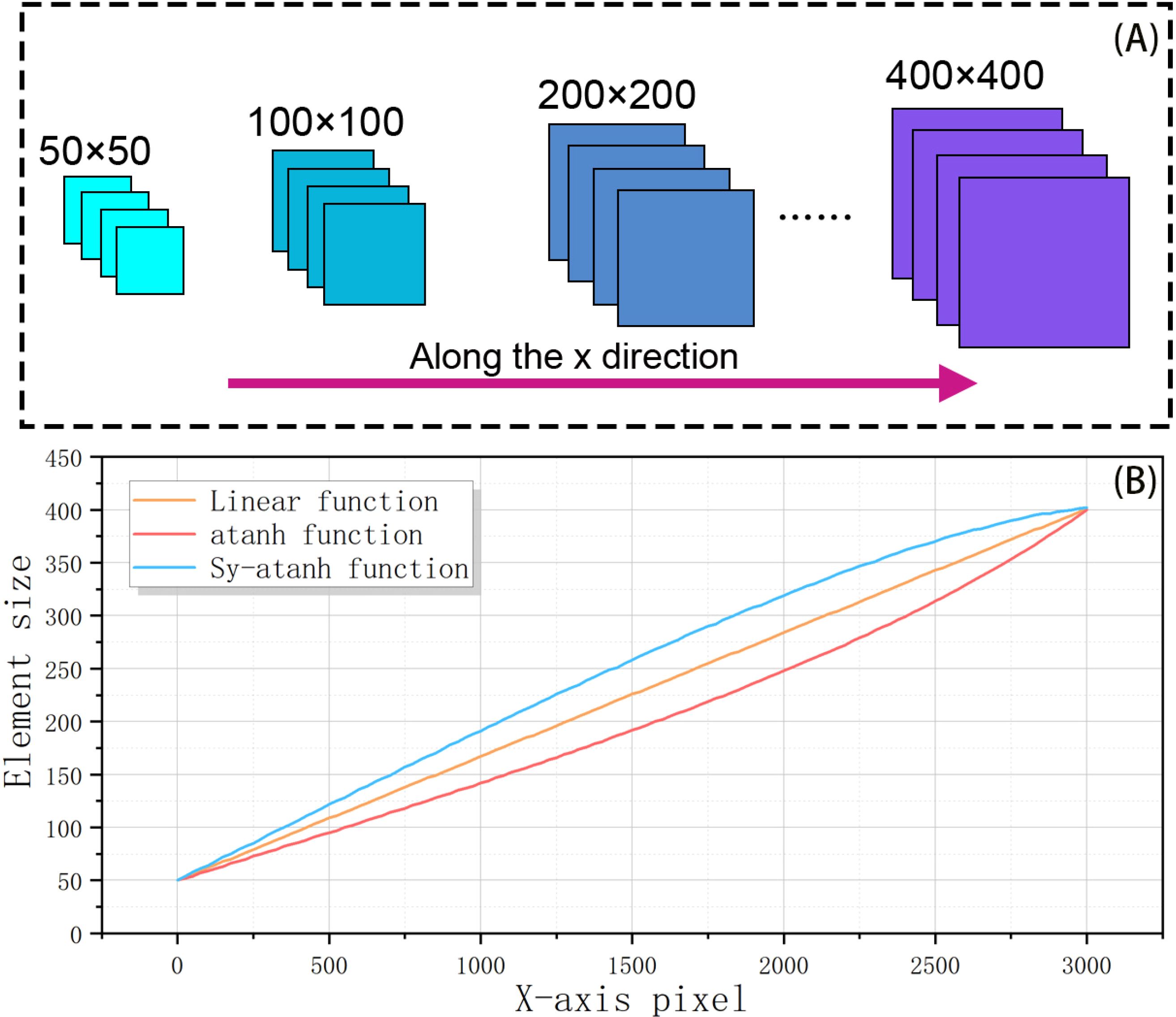
Figure 4. Remote sensing image segmentation method. (A) shows the result of segmentation along the x-direction at the coastline. (B) illustrates the curve that represents the variation in image element size with respect to x-pixels. This provides a detailed explanation of the fifth section in Figure 3.

2.2.5 Determining the image unit variation function

The relationship between wavelength and depth is nonlinear, and the depth characteristics vary in different areas. Thus, the image unit variation function can be diverse. An accurate variation function should align with the spatial variation in the swell wavelength, but determining this function is challenging because of the variable nature of wavelength information. Therefore, only an approximate variation function can be sought. However, a dynamic window is always more accurate and efficient than a fixed window. In this study, the image unit size variation from minimum to maximum is determined on the basis of three functions: a linear function, an atanh function, and a symmetric function of atanh with respect to the linear function(Sy-atanh). The choice of atanh is based on the relationship between depth and the swell wavelength, as illustrated in Figure 4B.

2.2.6 Window sliding

After determining the starting point on the coastline, image unit segmentation is performed along the x-direction of the coastline with a sliding step of 25 pixels. This step size is specifically chosen to address the challenge posed by the small coverage of high-resolution SAR images, which can affect the accuracy of depth inversion. By using a step size of 25 pixels, we aim to balance both the image resolution and the need for effective segmentation, ensuring that the method is robust enough to work with high-resolution images that have limited coverage. Once segmentation reaches the end of a segment, the next starting point is moved along the y-direction of the coastline, and steps 3-5 are repeated. For complex coastlines, an image unit expansion method is applied throughout the segmentation process to retrieve additional units as needed. This approach increases the utilization of image data near the coastline, helping to avoid inversion errors caused by the coastline intruding into image units during segmentation.

Due to the irregularity of coastlines, the wave-based method for depth inversion struggles with accurately segmenting images near the shore, leading to challenges in accurately inverting nearshore water depths. Typically, depth inversion areas are defined at a fixed distance from the coastline to overcome segmentation issues, or interpolation methods are used. However, these approaches often result in inaccurate depth inversion along the coastline. To address this challenge and improve the resolution of depth inversion, we propose a specialized method for handling starting points on the coastline. Taking Figure 5A as an example, the first step is to extract the coastline from the image, as shown in Figure 5B. After identifying the starting points along the coastline, we extend these points diagonally in both the upper-right and lower-right directions, thereby forming pixels that fully utilize the available image information. Next, we check whether the coastline intersects any newly formed pixels. If the coastline does intrude into the pixel area, we exclude these pixels from the depth inversion process, as illustrated in Figures 5C–E. By doing so, we ensure that only the most relevant regions, free from the interference of the coastline, are used for depth inversion. This approach enhances the resolution of depth inversion by accurately defining the region of interest near the coastline. It eliminates the inaccuracies introduced by interpolation or arbitrary distance-based segmentation and allows for more precise depth inversion, especially in areas where traditional methods struggle.

Figure 5

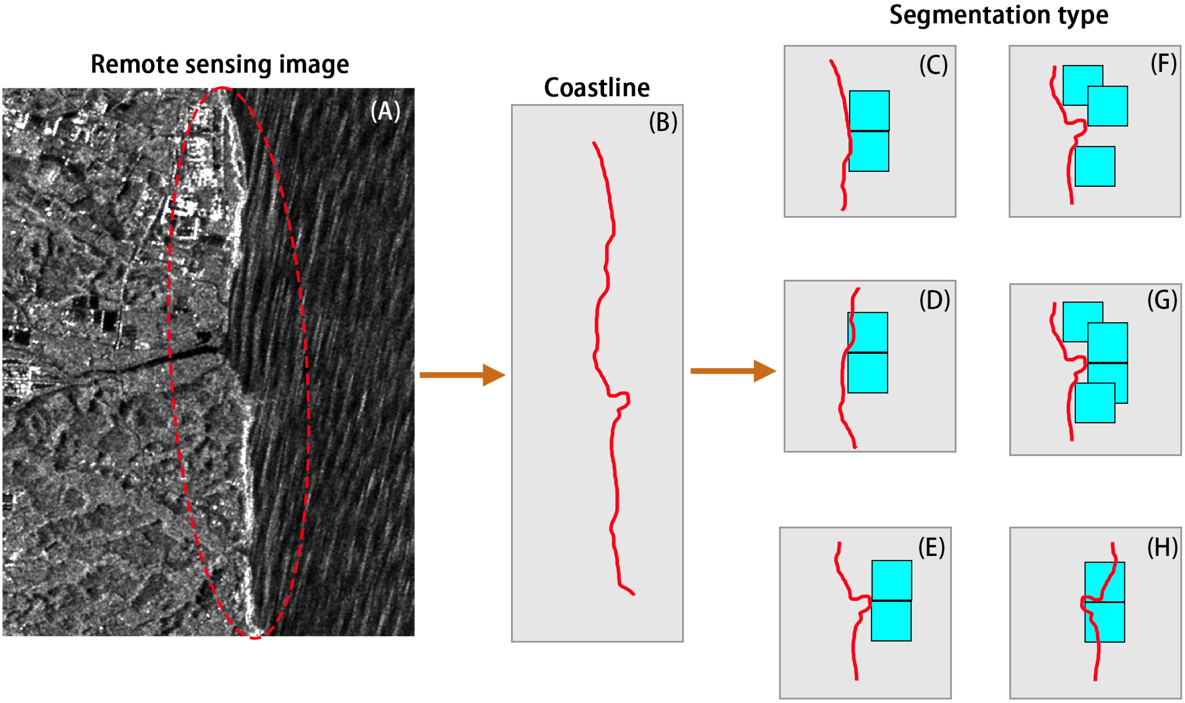
Figure 5. Coastal line processing method. Extracting the coastline from the remote sensing image in (A) yields (B). (C, D) depict two curved coastline segmentation methods. (E) shows the segmentation method where the coastline protrudes outward at the critical position. (F, G) illustrate how different segmentation methods for curved coastlines can lead to reduced resolution. (H) represents the segmentation method where the coastline concaves inward at the critical position.

Initially, to avoid the intrusion of the coastline into the pixels, we considered determining different extension methods according to the slope of the coastline. However, this approach results in segmentation gaps when there are corners in the coastline, as shown in Figure 5F. One potential solution involves allowing the starting points to extend upward and downward at the corners, but this requires identifying the corners, adding complexity to the process. Therefore, we adopted the approach of extending in two directions for each starting point pixel, which is more efficient and convenient. This method also effectively avoids introducing errors caused by the complete intrusion of the coastline, as shown in Figure 5H.

2.3 Theory of depth inversion methods

The theory of depth inversion based on wave dynamics, also referred to as linear wave theory or Airy theory, provides analytical solutions to the momentum and mass conservation equations that describe the velocity field and pressure along a water column. This theory establishes a relationship between wave speed, wave frequency, and water depth (the linear dispersion relationship) (Svendsen, 2006), which can be expressed as follows:

$\begin{array}{ll}\text{λ}={\text{λ}}_0\text{ tanh }(kh)& (1)\end{array}$

where ${\text{λ}}_0=g{T}^2/2\pi$, T is the wave period, ɡ is the acceleration due to gravity, k is the wavenumber, and h is the water depth. The influence of the mean flow is neglected in (1). The water depth is expressed as follows:

$\begin{array}{ll}h=\frac{\text{λ}}{2\pi }\text{atanh }(\text{λ}/{\text{λ}}_0)& (2)\end{array}$

Using the two-dimensional FFT, the wavelength of the pixels segmented in Section 3.1 is obtained while simultaneously recording the latitude and longitude information of the pixel centers (Santos et al., 2020). The wavelength information is then incorporated into (2) for depth inversion, and the inversion results are filtered via a Gaussian filter.

Equations 1, 2 show that the accuracy of λ₀ significantly influences the inversion results. When λ₀ is overestimated, the estimated depth h is typically too shallow; conversely, an underestimated λ₀ leads to an overestimation of h. The determination of λ₀ is inherently linked to the initial depth estimation. Inaccurate initial depth values can introduce substantial errors in the inversion process, particularly in deep-water regions. To minimize these errors, using multiple data sets and computing their average to determine the initial depth and λ₀ is common practice.

3 Results

3.1 Depth inversion results under fixed window segmentation

Initially, we selected six fixed window sizes for bathymetric inversion in the study area to observe the inaccuracies of fixed window inversion and to determine the appropriate range for the windows. Figures 6A–F show the wavelength calculation results for window sizes of 50, 100, 150, 200, 300, and 400 pixels, respectively. When the window is small, the wavelength resolution in shallow areas (near the coastline) is better, but it worsens as the distance from the coastline increases. This is clearly observed in the green area in Figure 6A. As the fixed window size increases, the wavelengths in areas far from the coast become more distinguishable. However, the wavelengths near the coast, while somewhat resolvable, are larger than those in the calculations with smaller windows.

Figure 6

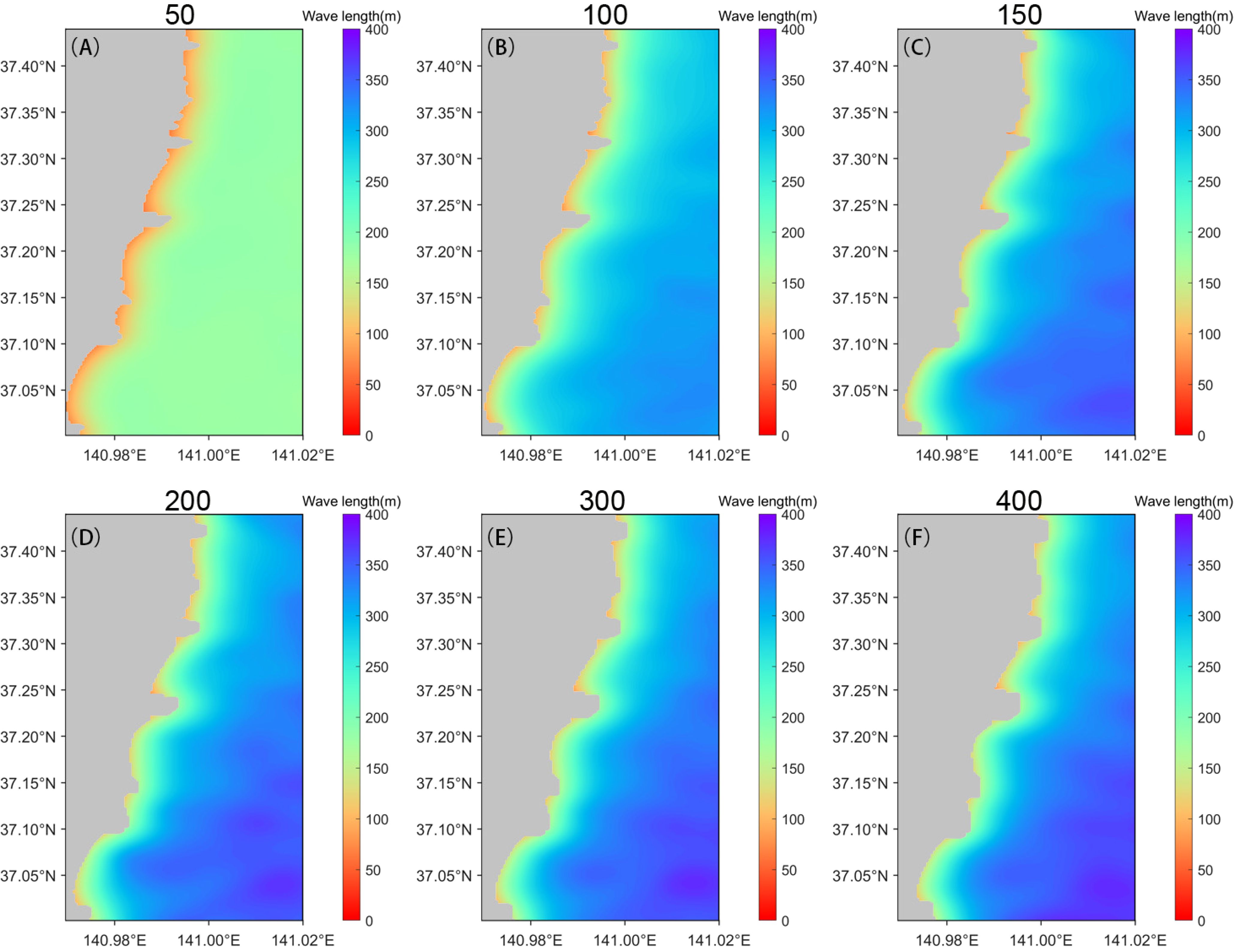
Figure 6. Wavelength inversion results are obtained through fixed-window processing. (A–F) display the results for varying window widths of 50, 100, 150, 200, 300, and 400 pixels, respectively. These different window sizes demonstrate the influence of spatial resolution on the accuracy and quality of wavelength inversion, emphasizing how the choice of window width can affect the precision of the results. Smaller window sizes are better suited for nearshore areas, while larger windows are more appropriate for offshore regions. However, a fixed window size is insufficient to accurately calculate surge wave wavelengths, particularly in cases where spatial variation is significant.

The wavelengths of swells near the coast are shorter and change more rapidly spatially. A larger window encompasses too much image information, including more wavelength data, which is evidently inaccurate for capturing nearshore swell wavelengths. Conversely, for areas far from the coast where swell wavelengths are longer, a small window might not even contain a complete wave period. Hence, smaller windows must be used near the coast, whereas larger windows are necessary farther offshore, underscoring the need for the dynamic window approach we propose.

Furthermore, as the window size increases, the left boundary of the calculation area shifts away from the coastline, significantly deforming the boundary line compared with the original coastline. This phenomenon is understandable, as the center points of windows near the coast move farther offshore as larger windows expand outward, causing the inversion area’s left boundary to shift rightward. The deformation occurs because larger windows, with fixed sliding steps, have greater distances between their center points, weakening the boundary resolution and deforming the coastline. This deformation does not occur with smaller windows. Additionally, our proposed outward expansion method was also applied with fixed windows. This method allows for the generation of an approximate irregular coastline even with unsuitable windows, whereas previous studies typically smoothed the bathymetry near the coastline into a curve.

We utilized (2) to perform depth inversion using the calculated wavelengths, and the inversion results are shown in Figure 7. Overall, the depth inversion results from smaller windows tend to be smaller. This is because in areas far from the coastline, where the wavelengths are smaller, fixed smaller wavelengths lead to overall smaller inversion results. As the window size increases, the water depth away from the coast gradually becomes more regular, and the range of water depths in the inversion increases, approaching the actual situation. However, issues in wavelength calculations persist in the depth inversion results.

Figure 7

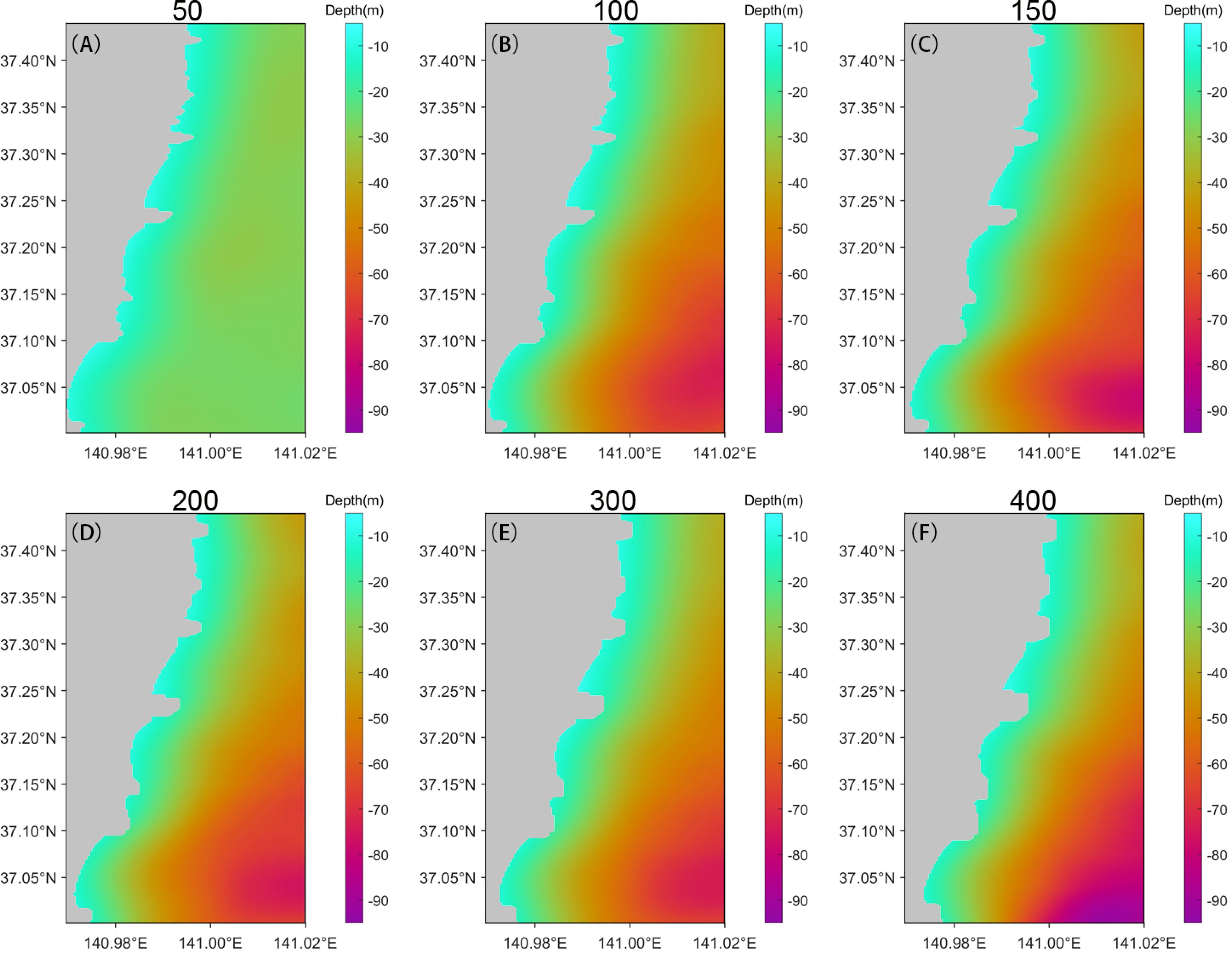
Figure 7. Water depth inversion results are obtained through fixed-window processing. (A–F) correspond to window widths of 50, 100, 150, 200, 300, and 400 pixels, respectively. The inverted water depth data clearly reflects the limitations of wave wavelength extraction using fixed windows. Smaller windows cannot capture information from deeper water, while larger windows may lead to data omission in nearshore areas. These results highlight the challenges of using a fixed window size for accurate water depth inversion across varying spatial scales.

Additionally, we observed that with larger window sizes, the spatial resolution of the inversion results decreases, which is more evident in the shape of the coastline. Therefore, the fixed window segmentation method inevitably introduces various issues, affecting both the inversion accuracy and spatial resolution. Moreover, manual judgment involvement in different segmentations of remote sensing images consumes considerable manpower and resources.

3.2 Depth inversion results using variable window segmentation

We also present the results of the wavelength calculation and depth inversion under the sliding variable window segmentation method employed in this study, as shown in Figure 8. The inversion results under the three types of window variation curves used in this study are closely aligned with the coastline identified in the remote sensing images, as the left boundary of the inversion area did not shift in all three cases. Compared with the fixed window segmentation method, the wavelengths obtained via the sliding variable window method are more suitable for each region of the entire area, as shown in Figures 8A–C. In the nearshore area, the wavelengths are smaller and gradually increase as we move away from the coastline. Additionally, the shape of the coastline remains unchanged under all three scenarios.

Figure 8

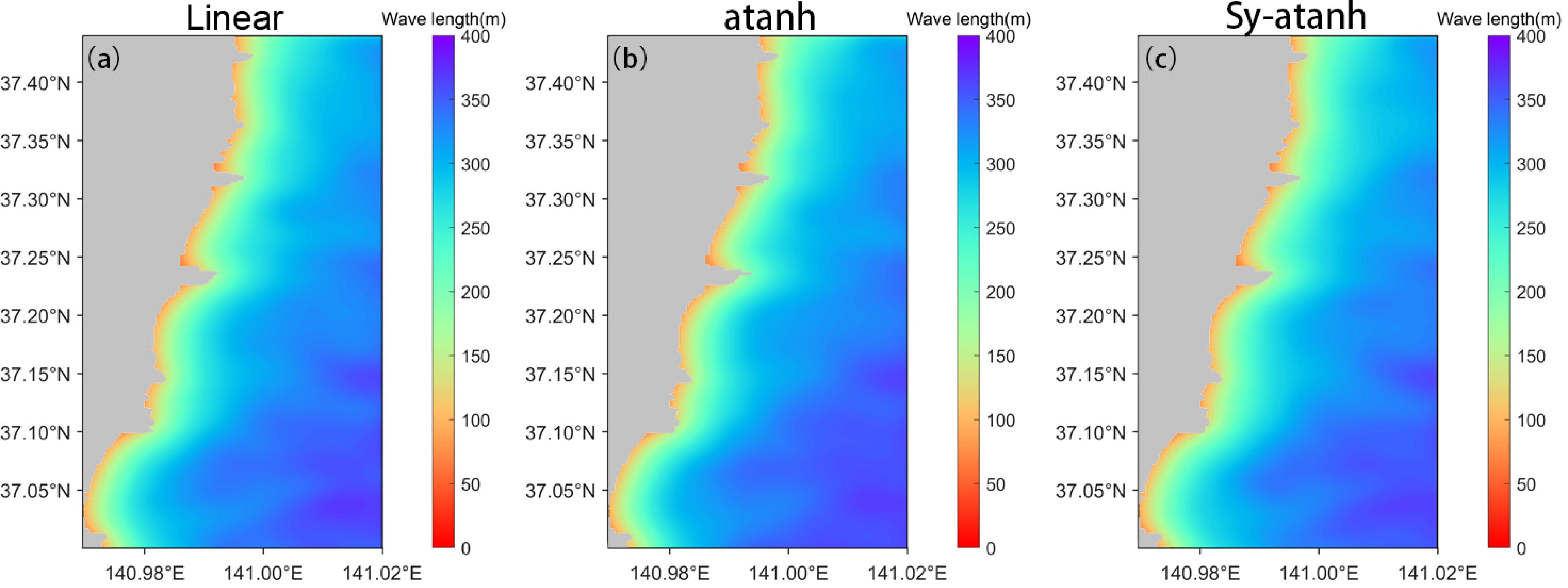
Figure 8. Wavelength inversion results after sliding window processing (A–C), and the functions used are Linear, atanh, and Sy-atanh, respectively.

Similarly, using (1) and (2), we derived the bathymetric distribution and compared it with the results obtained from fixed window sizes, as shown in Figure 9. Compared with those under small window segmentation, the inversion results under the three variation functions show clear depth resolution in areas far from the coast. Compared with those of larger windows, the inversion results under the three variation functions demonstrate higher resolution at the coastline, avoiding boundary shifts and maintaining good resolution.

Figure 9

Figure 9. Comparison of depth inversion results after fixed window processing (A–C) and sliding window processing (D–F). The results demonstrate that the sliding-window approach effectively addresses the limitations observed in the fixed-window method, providing more accurate water depth inversion across the entire area, particularly in nearshore regions. This improvement highlights the advantages of the sliding-window technique in overcoming spatial resolution challenges inherent to fixed-window processing.

Overall, the inversion results from the sliding segmentation with variable windows inherit the advantages of both small and large windows. The dynamic variable windows enable the segmented image to better adapt to the wavelength information of different regions. This results in bathymetric inversion with more pronounced spatial detail than fixed windows do. For example, the bathymetric changes in Figures 9A–C are smoother, whereas those in Figures 9D–F show noticeable differences, which we analyze in the following sections. While manually adjusting the window size is possible, it greatly depends on the operator’s expertise and is time-consuming, especially for wider swath images and long time series images. Therefore, our proposed method effectively addresses these issues.

The overall distribution of the water depth obtained is close to that of the Earth Topography One Arc-Minute Global Relief Model (ETOPO2022) data. However, the maximum spatial resolution of the water depth obtained in this study reaches 5.5 m, which is crucial for nearshore water depth inversion. To better illustrate the inversion’s reliability, we matched this study’s inversion results with the ETOPO2022 data because their spatial resolutions differ. As shown in Figure 10, the comparison between the two datasets reveals that the determination coefficient for all three inversion results is 0.98, with a root mean square error (RMSE) of less than 6 m, a mean relative error (MRE) of less than 14%, and a mean absolute error (MAE) of less than 5 m. The fit between the two datasets remains relatively stable for water depths less than 50 m. However, when the water depth exceeds 50 m, the inversion results of the linear function curve tend to be underestimated. In contrast, those of the symmetric atanh function curve tend to be overestimated. Only the inversion results of the atanh function curve exhibit a slightly better fit than the other two, with the smallest RMSE and MRE among the three, at 4.8 m and 9.8%, respectively. Previous depth inversion methods have been difficult to verify on a large scale, with MREs typically between 10% and 30% (Pleskachevsky et al., 2011; Santos et al., 2021; Pereira et al., 2019). The spatial resolution typically ranges from hundreds of m to kilometers, making remote sensing data near coastlines nearly unusable. In comparison, our proposed method is efficient, has high precision, and offers high utilization.

Figure 10

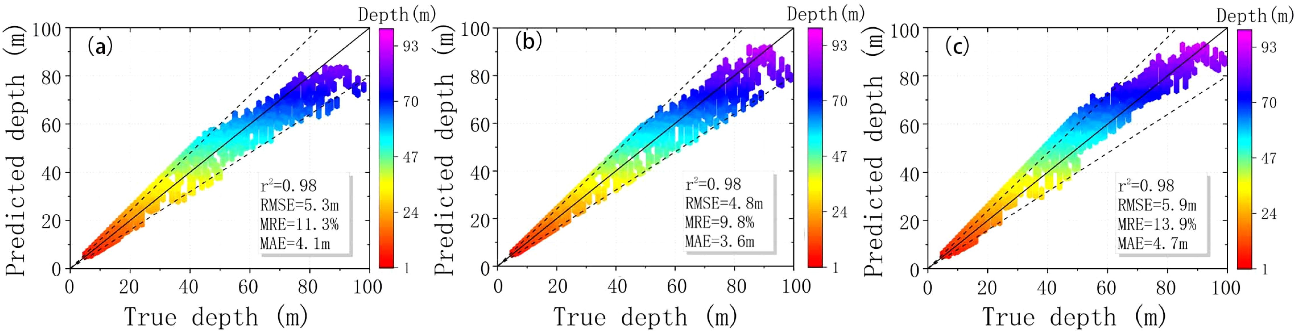
Figure 10. Comparison of depth inversion results after sliding window processing and ETOPO2022 data. The functions used are Linear (A), atanh (B), and Sy-ATANH (C).

To observe the inversion capability of this method across different water depths, we divided the inversion results into ranges with intervals of 20 m, ranging from 1 to 100 m. The specific errors are shown in Table 1. Concerning the relative error, the inversion results under the three window change functions exhibited significant relative errors between 20 m and 60 m, as depicted in Figure 11A. Among them, the inversion results of the symmetric atanh function were the poorest, showing unstable inversion capabilities with significant variations in relative error. Conversely, the results obtained from the linear function and atanh were relatively close. With respect to the absolute error, as shown in Figure 11B, as the water depth increased, the absolute error of the inversion results from the linear function gradually increased. However, for symmetric atanh and atanh, their absolute errors decreased gradually for water depths exceeding 60 m. Overall, the results obtained from the atanh function corresponding to the window transformation yielded slightly better outcomes, as evident from the variation curve of the RMSE in Figure 11C.

Table 1

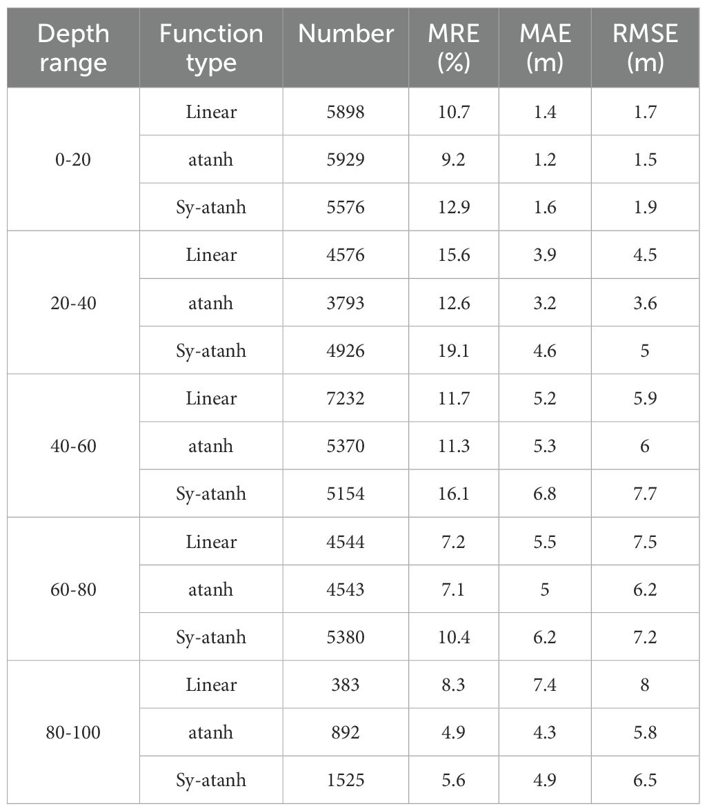
Table 1. The specific inversion results of the three variation functions at different depth ranges.

Figure 11

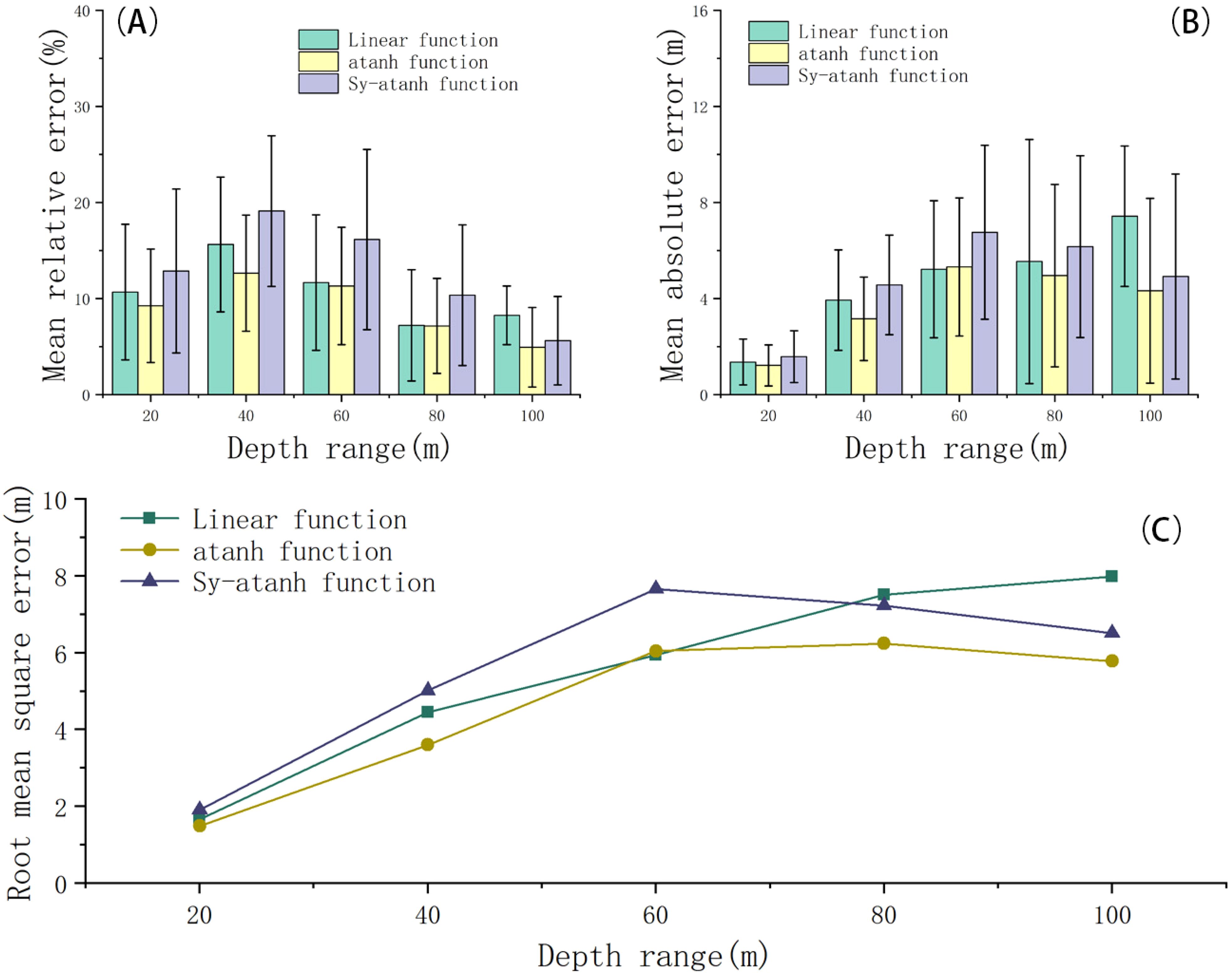
Figure 11. Analysis of the error in water depth inversion after sliding window processing. (A, B) show the MRE and MAE in different water depth ranges, with the numerical value on the horizontal axis representing the end point of the water depth range. (C) shows the RMSE of the water depth inversion in different water depths.

To further analyze the inversion results, we isolate the inversion results segmented by the atanh function curve window transformation. After the spatial resolution is reduced, the overall consistency between the inversion results and the ETOPO2022 data becomes more evident, as shown in Figures 12A, B. Statistical analysis revealed that the maximum water depth in the study area is 92 m, and the minimum depth is 5 m, with an average depth of 37 m, as shown in Figure 12C. The values are distributed mainly between 10 m and 50 m. Notably, the quantity of inverted values is related to both the characteristics of the water depth distribution in the study area and the properties of the window. The deeper the water depth is, the larger the data interval and the larger the window. Overall, the northern part of the study area has relatively shallow water depths, primarily within 50 m. In contrast, the southern part experiences drastic changes in water depth, gradually approaching the Japan Trench.

Figure 12

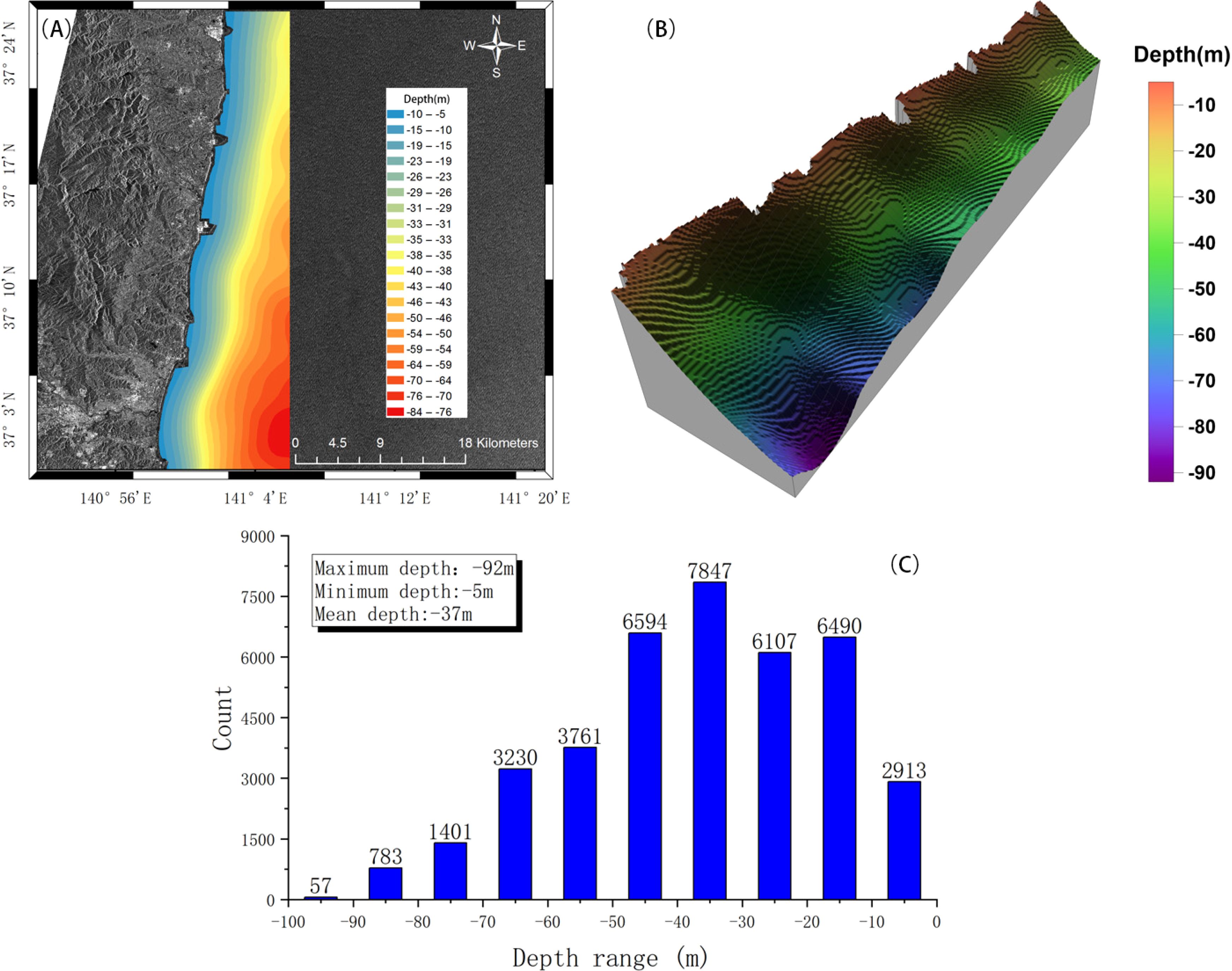
Figure 12. Water depth distribution (A) and three-dimensional representation of water depth (B) under the atanh segmentation function. (C) shows the numerical statistics of the water depth.

4 Discussion

We calculated the gradient of water depth changes to demonstrate variations in the inversion results. As shown in Figure 13A, the gradient of the water depth along the east–west direction reveals a distinct band of intense depth changes not far from the shore (enclosed by the solid green line in Figure 13A), where the maximum depth gradient reaches 9.2 m per kilometer. Additionally, in the southeastern region of the study area, two circular areas with significant gradients are observed (enclosed by the solid blue circles in Figure 13A). Moreover, the changes in the north–south gradient in the inversion results are relatively small, as depicted in Figure 13B. However, within the band of intense east–west gradient changes, three regions with significant north–south gradient changes are identified (enclosed by the dashed green lines in Figure 13B). The two regions with pronounced north–south gradient changes are consistent with the locations of the circular depressions shown in Figure 12C, which are more readily observable because of the reduced resolution in Figure 12A. This highlights the importance of enhancing spatial resolution in remote-sensing-based inversions. The appearance of these depressions may be related to underwater seismic activity (Booth et al., 2020), which requires further investigation.

Figure 13

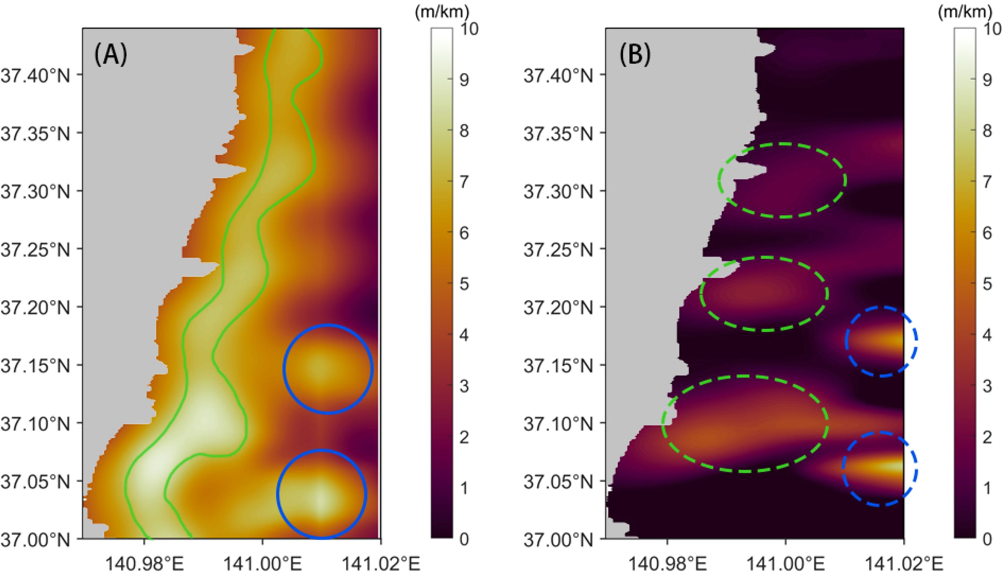
Figure 13. Variation in the water depth gradient in the east–west direction (A) and north–south direction (B). The green solid and dashed lines enclose the regions with relatively large gradients near the coastline. The blue solid and dashed lines enclose the regions with relatively large gradients far from the coastline.

In fact, the SAR bathymetric inversion method proposed in this paper has broad applications in real-world scenarios, including coastal management, maritime navigation, and disaster response. High-precision SAR bathymetric inversion technology can be used for regular monitoring of coastline depth changes, thereby assessing beach erosion and accretion. For example, in areas prone to erosion, this technology can help managers identify severely eroded regions and develop protective strategies accordingly. Additionally, in maritime navigation, high-precision SAR bathymetric inversion technology can be used for route planning and obstacle detection, accurately measuring channel depths to ensure that vessels avoid shallow areas and underwater reefs during navigation.

The dynamic window sliding segmentation method proposed in this paper is our preliminary work, and we will further refine it in future studies. By dynamically adjusting the window size, we have enhanced the accuracy of bathymetric inversion and increased the method’s utilization and resolution of remote sensing images through outward expansion. However, there is no universally applicable method for determining the variation function, and we have only conducted preliminary attempts, considering the varying depth and wavelength distributions in different marine areas. This, we believe, is a key factor in further improving the inversion accuracy and resolution.

In future work, integrating optical methods with SAR inversion for multisource data fusion presents several challenges that need to be addressed. One major challenge is the difference in the types of information provided by each sensor. SAR data, which captures surface characteristics and dynamics, often struggles with shallow water due to surface roughness and wave effects. In contrast, optical imagery provides high spatial resolution and can capture underwater features directly in clear water but is limited by environmental conditions such as cloud cover and water turbidity. Thus, combining these two data sources requires careful alignment of the information extracted from each sensor type. To address this, one potential solution is the development of advanced fusion algorithms that can effectively combine the complementary strengths of both datasets. These algorithms should account for differences in resolution, spectral range, and environmental sensitivities. For example, SAR data can provide detailed surface information, while optical data can improve the accuracy of bathymetric models by filling in gaps in the shallow-water depths and providing higher resolution for the seafloor. Another challenge is the need for robust data preprocessing to correct various distortions and discrepancies between the data sources. Techniques like image registration, normalization, and co-registration will be critical in accurately aligning the SAR and optical images.

5 Conclusions

This study addresses critical challenges in SAR-based depth inversion techniques and proposes a method based on variable window image element segmentation. This method significantly enhances the accuracy and efficiency of depth inversion in regions with complex underwater terrain. Through an analysis of SAR images along the coast of Naraha, we successfully extracted accurate wavelength information and derived water depth distributions via linear dispersion relationships. Compared with traditional fixed window size segmentation methods, the variable window image segmentation method can more accurately adapt to changes in wave characteristics under different water depth conditions, thus improving the accuracy of depth inversion. The coast of Naraha, characterized by frequent geological activity and complex water depth variations, demands greater precision and reliability in depth inversion techniques. The method adopted in this study enables effective depth detection in regions with irregular coastlines and uneven underwater terrain, with RMSE and MRE values of 4.8 m and 9.8%, respectively, and a maximum spatial resolution of 5.5 m. This provides new technological support for marine mapping, marine resource exploration, and ocean environmental monitoring. Furthermore, the results of this study further validate the feasibility of depth inversion on the basis of wave characteristics and linear dispersion relationships, expanding the application scope of SAR technology in marine science. With the continuous development of spaceborne SAR technology and the acquisition of more high-resolution SAR satellite data, we believe that SAR depth inversion methods based on variable window image element segmentation will play a more critical role in future ocean exploration, providing more accurate and reliable data support for scientific marine research. In future, further improvements in segmentation algorithms and the integration of multisource data could enhance depth inversion in more challenging environments. Additionally, the development of automated, real-time depth inversion systems for large-scale monitoring could broaden the applicability of this method.

Data availability statement

The datasets presented in this study can be found in online repositories. The names of the repository/repositories and accession number(s) can be found in the article/supplementary material.

Author contributions

MZ: Writing – original draft, Methodology, Software, Validation. CQ: Writing – original draft, Methodology, Validation. FY: Writing – review & editing, Formal Analysis, Methodology. RW: Writing – review & editing, Methodology, Validation. SP: Writing – review & editing, Formal Analysis.

Funding

The author(s) declare financial support was received for the research, authorship, and/or publication of this article. This work was supported by the Natural Science Foundation of Shandong Province under Grant ZR2022MD002, the National Natural Science Foundation of China under Grant 42304051 and 41930535, and the Hainan Province Science and Technology Special Fund under Grant ZDYF2023GXJS005.

Acknowledgments

The authors would like to acknowledge the provision of GF-3 images by the China Centre for Resources Satellite Data and Application.

Conflict of interest

The authors declare that the research was conducted in the absence of any commercial or financial relationships that could be construed as a potential conflict of interest.

Generative AI statement

The author(s) declare that no Generative AI was used in the creation of this manuscript.

Publisher’s note

All claims expressed in this article are solely those of the authors and do not necessarily represent those of their affiliated organizations, or those of the publisher, the editors and the reviewers. Any product that may be evaluated in this article, or claim that may be made by its manufacturer, is not guaranteed or endorsed by the publisher.

References

Alpers W., Hennings I. (1984). A theory of the imaging mechanism of underwater bottom topography by real and synthetic aperture radar. J. Geophysical Res. 89, 10529. doi: 10.1029/JC089iC06p10529

Crossref Full Text | Google Scholar

Bian X., Shao Y., Tian W., Zhang C. Y. (2016). Estimation of shallow water depth using hj-1c s-band sar data. J. Navigation 69, 113–126. doi: 10.1017/S0373463315000454

Crossref Full Text | Google Scholar

Bian X., Shao Y., Zhang C. Y., Xie C., Tian W. (2020). The feasibility of assessing swell-based bathymetry using sar imagery from orbiting satellites. ISPRS J. Photogrammetry Remote Sens. 168, 124–130. doi: 10.1016/j.isprsjprs.2020.08.006

Crossref Full Text | Google Scholar

Boccia V., Renga A., Rufino G., D'Errico M., Moccia A., Aragno C., et al. (2015). Linear dispersion relation and depth sensitivity to swell parameters: Application to synthetic aperture radar imaging and bathymetry. Sci. World J. 2015, 374579. doi: 10.1155/tswj.v2015.1

PubMed Abstract | Crossref Full Text | Google Scholar

Booth S., Walters W. J., Steenbeek J., Christensen V., Charmasson S. (2020). An ecopath with ecosim model for the pacific coast of eastern Japan: Describing the marine environment and its fisheries prior to the great east Japan earthquake. Ecol. Model. 428, 109087. doi: 10.1016/j.ecolmodel.2020.109087

Crossref Full Text | Google Scholar

Brusch S., Held P., Lehner S., Rosenthal W., Pleskachevsky A. (2011). Underwater bottom topography in coastal areas from terrasar-x data. Int. J. Remote Sens. 32, 4527–4543. doi: 10.1080/01431161.2010.489063

Crossref Full Text | Google Scholar

Cao C., Bao L., Gao G., Liu G., Zhang X. (2024). A novel method for ocean wave spectra retrieval using deep learning from sentinel-1 wave mode data. IEEE Trans. Geosci. Remote Sens. 62, 4204016. doi: 10.1109/TGRS.2024.3369080

Crossref Full Text | Google Scholar

de Michele M., Raucoules D., Idier D., Smai F., Foumelis M. (2021). Shallow bathymetry from multiple sentinel 2 images via the joint estimation of wave celerity and wavelength. Remote Sens.13, 2149. doi: 10.3390/rs13112149

Crossref Full Text | Google Scholar

Fan K. G., Huang W. G., He M. X., Fu B., Zhang B., Chen X. Y. (2008). Depth inversion in coastal water based on sar image of waves. Chin. J. Oceanology Limnology 26, 434–439. doi: 10.1007/s00343-008-0434-4

Crossref Full Text | Google Scholar

Huang W. G., Fu B., Zhou C. B., Yang J. S., Shi A. Q., Li D. L. (2000). Simulation study on optimal currents and winds for the spaceborne sar mapping of sea bottom topography. Prog. Nat. Sci. 10, 859–866. doi: 10.1007/s002690000111

Crossref Full Text | Google Scholar

Huang L. Y., Yang J. G., Meng J. M., Zhang J. (2021). Underwater topography detection and analysis of the qilianyu islands in the south China sea based on gf-3 sar images. Remote Sens. 13, 76. doi: 10.3390/rs13010076

Crossref Full Text | Google Scholar

Jay S., Guillaume M. (2016). Regularized estimation of bathymetry and water quality using hyperspectral remote sensing. Int. J. Remote Sens. 37, 263–289. doi: 10.1080/01431161.2015.1125551

Crossref Full Text | Google Scholar

Li X., Li C., Xu Q., Pichel W G. (2009). Sea surface manifestation of along-tidal-channel underwater ridges imaged by sar. IEEE Trans. Geosci. Remote Sens. 47, 2467–2477. doi: 10.1109/TGRS.2009.2014154

Crossref Full Text | Google Scholar

Liang R., Dai K., Xu Q., Pirasteh S., Li Z., Wen N., et al. (2024). Utilizing a single-temporal full polarimetric gaofen-3 sar image to map coseismic landslide inventory following the 2017 mw 7.0 jiuzhaigou earthquake (China). Int. J. Appl. Earth Observation Geoinformation 127, 103657. doi: 10.1016/j.jag.2024.103657

Crossref Full Text | Google Scholar

Loor G. (1981). The observation of tidal patterns, currents, and bathymetry with slar imagery of the sea. IEEE J. Oceanic Eng. 6, 124–129. doi: 10.1109/JOE.1981.1145501

Crossref Full Text | Google Scholar

Loor G. P., Hulten H. (1978). Microwave measurements over the north sea. Boundary-Layer Meteorology 13, 119–131. doi: 10.1007/BF00913866

Crossref Full Text | Google Scholar

Mao W., Liu G., Wang X., Yakun X., He X., Zhang B., et al. (2022). Using range split-spectrum interferometry to overcome phase unwrapping errors for insar-derived dem. Remote Sens.14, 2607. doi: 10.3390/rs14112607

Crossref Full Text | Google Scholar

Mao W., Wang X., Liu G., Zhang R., Shi Y., Pirasteh S. (2021). Estimation and compensation of ionospheric phase delay for multi-aperture insar: an azimuth split-spectrum interferometry method. IEEE Trans. Geosci. Remote Sens. 60, 1–14. doi: 10.1109/TGRS.2021.3095272

Crossref Full Text | Google Scholar

McLeish W., Swift D. J. P., Long R. B., Ross D., Merrill G. (1981). Ocean surface patterns above sea-floor bedforms as recorded by radar, southern bight of north sea. Mar. Geology 43, M1–M8. doi: 10.1016/0025-3227(81)90121-3

Crossref Full Text | Google Scholar

Mishra M. K., Ganguly D., Chauhan P., Ajai. (2014). Estimation of coastal bathymetry using risat-1 c-band microwave sar data. IEEE Geosci. Remote Sens. Lett. 11, 671–675. doi: 10.1109/LGRS.2013.2274475

Crossref Full Text | Google Scholar

Misra A., Ramakrishnan B., Muslim A. M. (2020). Synergistic utilization of optical and microwave satellite data for coastal bathymetry estimation. Geocarto Int. 37 (8), 2323–2345. doi: 10.1080/10106049.2020.1829100

Crossref Full Text | Google Scholar

Pereira P., Baptista P., Cunha T., Silva P. A., Romao S., Lafon V., et al. (2019). Estimation of the nearshore bathymetry from high temporal resolution sentinel-1a c-band sar data - a case study. Remote Sens. Environ. 223, 166–178. doi: 10.1016/j.rse.2019.01.003

Crossref Full Text | Google Scholar

Pleskachevsky A., Lehner S., Heege T., Mott C. (2011). Synergy and fusion of optical and synthetic aperture radar satellite data for underwater topography estimation in coastal areas. Ocean Dynamics 61, 2099–2120. doi: 10.1007/s10236-011-0460-1

Crossref Full Text | Google Scholar

Qi C., Wang X. K., Su D. P., Guo Y. D., Yang F. L. (2023). Comparison and analysis of ground seed detectors and interpolation methods in airborne lidar filtering. Egyptian J. Remote Sens. Space Sci. 26, 1009–1019. doi: 10.1016/j.ejrs.2023.10.004

Crossref Full Text | Google Scholar

Santos D., Abreu T., Silva P. A., Baptista P (2020). Estimation of coastal bathymetry using wavelets. J. Mar. Sci. Eng. 8, 172. doi: 10.3390/jmse8100772

Crossref Full Text | Google Scholar

Santos D., Fernández-Fernández S., Abreu T., Silva P. A., Baptista P., et al. (2021). Retrieval of nearshore bathymetry from sentinel-1 sar data in high energetic wave coasts: The portuguese case study. Remote Sens. Applications: Soc. Environ. 25, 100674c. doi: 10.1016/j.rsase.2021.100674

Crossref Full Text | Google Scholar

Shuchman R. A., Lyzenga D. R., Meadows G. A. (1985). Synthetic aperture radar imaging of ocean-bottom topography via tidal-current interactions: theory and observations. Int. J. Remote Sens. 6, 1179–1200. doi: 10.1080/01431168508948271

Crossref Full Text | Google Scholar

Svendsen I. A. (2006). Introduction to nearshore hydrodynamics Vol. 24 (New Jersey: World Scientific).

Google Scholar

Valenzuela G. R., Chen D. T., Garrett W. D., Kaiser J. A. C. (1983). Shallow water bottom topography from radar imagery. Nature 303, 687–689. doi: 10.1038/303687a0

Crossref Full Text | Google Scholar

Wang X. K., Yang F. L., Zhang H. D., Su D. P., Wang Z. L., Xu F. Z. (2022). Registration of airborne lidar bathymetry and multibeam echo sounder point clouds. IEEE Geosci. Remote Sens. Lett. 19, 6501605. doi: 10.1109/LGRS.2021.3076462

Crossref Full Text | Google Scholar

Wu L. H., Xu W. H., Wang W. (2013). Survey of seafloor targets with varied sizes by multi beam sonar in different depth water. Appl. Mechanics Materials 263-266, 909–914. doi: 10.4028/www.scientific.net/AMM.263-266.909

Crossref Full Text | Google Scholar

Yang F. L., Qi C., Su D. P., Ma Y., He Y., Wang X. H., et al. (2023). Modeling and analyzing water column forward scattering effect on airborne lidar bathymetry. IEEE J. Oceanic Eng. 48, 1373–1388. doi: 10.1109/JOE.2023.3275695

Crossref Full Text | Google Scholar

Zhang X., Gao G., Chen S. W. (2024b). Polarimetric autocorrelation matrix: A new tool for joint characterizing of target polarization and doppler scattering mechanism. IEEE Trans. Geosci. Remote Sens. 62, 5213522. doi: 10.1109/TGRS.2024.3398632

Crossref Full Text | Google Scholar

Zhang C., Zhang X., Gao G., Lang H. T., Liu G. W., Song Y. Y., et al. (2024a). Development and application of ship detection and classification datasets: a review. IEEE Geosci. Remote Sens. Magazine 12 (4), 12–45. doi: 10.1109/MGRS.2024.3450681

Crossref Full Text | Google Scholar

Zheng Q., Li L., Guo X. G., Ge Y., Zhu D. Y., Li C. Y., et al. (2006). Sar imaging and hydrodynamic analysis of ocean bottom topographic waves. J. Geophysical Research: Oceans 111, C09028. doi: 10.1029/2006JC003586

Crossref Full Text | Google Scholar

Zheng Q., Zhao Q., Yuan Y., Liu X., Hu J. Y., Liu X. H., et al. (2012). Shear-flow induced secondary circulation in parallel underwater topographic corrugation and its application to satellite image interpretation. J. Ocean Univ. China 11, 427–435. doi: 10.1007/s11802-012-2093-5

Crossref Full Text | Google Scholar

Zhou H., Dai K., Pirasteh S., Li R., Xiang J., Li Z. (2023). Insar spatial-heterogeneity tropospheric delay correction in steep mountainous areas based on deep learning for landslides monitoring. IEEE Trans. Geosci. Remote Sens. 61, 5215014. doi: 10.1109/TGRS.2023.3307477

Crossref Full Text | Google Scholar