An updated regional model skill assessment for seasonal and interannual variability of bottom temperature across the eastern Bering Sea shelf

The Bering10K Regional Ocean Modeling System (ROMS) model is a high-resolution (10-km) regional ocean model that has been used over the past decade to investigate relationships between the physical environment and the eastern Bering Sea shelf ecosystem in both research and management contexts. Extensive validation for this model has been conducted previously, particularly focused on bottom temperature, a key physical driver shaping ecosystem dynamics in this region. However, previous observations of bottom temperature were primarily limited to the summer months. Recent deployments of pop-up floats capable of overwinter measurements now allow us to extend the previous validation to other seasons. Here, we characterize bottom temperature on the southeastern Bering Sea shelf across time scales by combining data from our new pop-up floats with several existing temperature datasets. We then use this combination of data to systematically assess the skill of the Bering10K ROMS model in capturing these features, focusing on spatial variability in skill metrics and the potential processes leading to these patterns. We confirm that the model captures shelf-wide patterns in bottom temperature well, including mean patterns as well as both seasonal and interannual variability. However, a few areas of potential improvement were also identified: underestimated surface mixing in the model leads to delayed destratification across the middle and outer shelves, the position of the inner front may be offset slightly in the model, and bathymetric smoothing leads to poor representation near the shelf break and potentially underestimated flow onto the shelf through shelf break canyons. Overall, this paper presents the most detailed spatiotemporal analysis of this model’s skill in simulating bottom temperature across the eastern Bering Sea shelf to date and supplies a benchmark analysis framework that can be used for planned regional model transitions and improvements over the coming years.

1 Introduction

Regional ocean models are increasingly being used for ecosystem-based management applications related to fisheries and other living marine resources. These tools can offer increased spatial and temporal coverage beyond that available through in situ and satellite data products, allowing better understanding of the potential connections between environmental variables and ecosystem metrics of interest. They also offer the ability to forecast, assisting in both short-term management decisions and long-term planning in the face of climate change. To be useful, these models require extensive validation to demonstrate their ability to capture the biophysical processes relevant to the ecosystem questions being investigated. Model validation typically begins with a focus on large-scale patterns across regional domains. However, as the models are used to investigate increasingly complex and nuanced questions, so too must the skill assessment of the model delve into these nuances.

The eastern Bering Sea shelf is a highly productive region. Despite its northern latitude, the geometry of the wide, shallow shelf results in a long growing season with high productivity supporting both pelagic and benthic communities (Rho and Whitledge, 2007). This in turn supports large commercial and subsistence fisheries. This region is characterized by seasonal sea ice that covers much of the shelf during the winter months. Sea ice formation processes lead to the creation of a characteristic pool of cold bottom water (<2°C) across much of the shelf (Stabeno et al., 2001). In particular, the middle shelf region between the 50 m and 100 m isobaths experiences strong seasonal stratification in the summer, with a sharply stratified two-layer system of warmer surface waters and cold bottom water. Because of their relationship with both direct and indirect drivers of fish recruitment and survival, indices of bottom temperature and cold pool extent are commonly used as ecosystem indicators and environmental covariates in fisheries and ecosystem management activities in the region (e.g., O’Leary et al., 2020; Thorson et al., 2021; Siddon, 2023). Historically, these were primarily calculated based on in situ measurements collected during the annual Bering Sea groundfish survey. However, in recent years, temperature output from a regional ocean model, a Regional Ocean Modeling System (ROMS) implementation with 10-km horizontal resolution that is designated here as “Bering10K”, has also been used to supplement these observations. In particular, a reanalysis-driven hindcast simulation spanning 1970–present is updated twice per year to provide additional spatiotemporal information regarding early spring through late summer conditions (Siddon, 2023). A similar model configuration has been used to investigate management adaptation strategies to mitigate potential climate change impacts over the next century (Hollowed et al., 2020).

The Bering10K model has undergone extensive validation to demonstrate that it successfully captures the biophysical features necessary to be used in these management contexts (Kearney et al., 2020; Kearney, 2021). The initial phase of validation relied primarily on satellite data and summer in situ data since the large spatial extent, remote location, and presence of seasonal sea ice limit the opportunities to collect data outside of the spring and summer months. It also focused primarily on shelf-wide indices that would be most relevant to the Bering Sea ecosystem as a whole. However, given the model’s success in this context, there is now interest in using it to address species-specific and life-stage-specific questions that require knowledge of environmental conditions during the observationally sparse winter and spring months. For example, Pacific cod (Gadus macrocephalus) are sub-Arctic gadids that have historically favored the warmer portions of the Bering Sea shelf, that is, the southern portions outside the core cold pool location (Barbeaux and Hollowed, 2018). But during recent low-sea-ice years in 2018 and 2019 with near-absent cold pool conditions, these fish appeared to move poleward during the summer (Stevenson and Lauth, 2019). Pacific cod eggs, which are released on the bottom during the spring, require narrow temperature ranges (3–6°C) during their development (Laurel and Rogers, 2020; Bian et al., 2016). Ongoing research is attempting to address the question of whether future warm conditions may lead to a shift in spawning habitat in addition to allowing for expanded adult migration.

This use case highlights the need for more in-depth validation of the Bering10K model. To date, the limited spatiotemporal coverage of historical data has hampered our ability to assess performance of the Bering10K model year-round, particularly during the winter and spring months when the cold pool is formed and begins its decay. This limits our confidence in using Bering10K outputs for studies of winter ecology, such as spawning habitat suitability for Pacific cod. However, recent deployments of new instruments known as pop-up floats (PUFs) are helping to fill this gap. These floats are anchored to the seafloor for a set period of time to collect data, then are released, float to the surface, and transmit their data. This allows for temperature data to be collected over the winter months, including during periods of ice cover.

The addition of these new time series offers an opportunity to bring together bottom temperature data from these new popup-floats alongside existing observational datasets and our Bering10K hindcast simulation to 1) assess model skill in more spatiotemporal detail and 2) use model skill statistics to better form a cohesive understanding of temperature dynamics and cold pool evolution across the Bering Sea shelf. This assessment will also allow us to identify remaining knowledge gaps in the dynamics of the shelf and our ability to simulate them.

In this paper, we characterize bottom temperature on the southeastern Bering Sea shelf across time scales — including mean state, seasonal evolution, and interannual variability of the cold pool — by combining data from our new pop-up floats with several existing datasets. We then use this combination of data to evaluate the skill of the Bering10K ROMS model in capturing bottom temperature across different spatial and temporal scales. By combining datasets with contrasting spatiotemporal coverage, we are able to advance our understanding of the physical processes that underlie bottom temperature patterns, diagnose whether our existing model captures those processes, and propose potential improvements to the model where skill is lacking.

We present our analysis in several stages. We begin by expanding upon a previous skill analysis (Kearney, 2021) that uses temperature data from the yearly eastern Bering Sea continental shelf groundfish survey to assess the model’s ability to capture interannual-scale variability in summer bottom temperature. This dataset provides a 40-year time series of spatially-resolved data across the southeastern shelf, but is limited to summer data only. With this updated summer-only skill assessment as our baseline, we then divide the shelf into several regions based on similarity of metrics. We use the newly collected pop-up float data alongside existing mooring data to evaluate whether those metrics hold for the seasonal evolution of bottom temperatures and to further elucidate the mechanisms driving these patterns. Given the sequential and descriptive nature of this analysis, we structure this paper with a Methods section to describe the regional model setup, bottom temperature collection methods, and baseline skill statistics calculations and then combine the Results and Discussion sections as we step through the regional analyses.

2 Methods

2.1 The Bering10K regional model

The Bering10K regional model is an implementation of the Regional Ocean Modeling System (ROMS, Shchepetkin and McWilliams, 2005; Haidvogel et al., 2008). Its domain covers the Bering Sea and northeast Gulf of Alaska (Figure 1), with 10-km horizontal resolution and 30 terrain-following depth levels. Vertical mixing follows the algorithms of Large et al. (1994), with explicit inclusion of tidal dynamics to allow for tidally-generated mixing and tidal residual flows. Sea ice dynamics combine elastic-viscous-plastic rheology with a one-layer ice and snow thermodynamics model (Budgell, 2005). For the hindcast simulations used in this study, boundary conditions and atmospheric forcing are provided by reanalysis-based datasets, including the Common Ocean Reference Experiment (Large and Yeager, 2009) from 1970–1994, Climate Forecast System Reanalysis from 1995–March 2011 (Saha et al., 2010), and Climate Forecast System Operational Analysis from April 2011–Aug 2023 (Saha et al., 2014). Freshwater runoff was reconstructed from observed river discharge from Alaskan and Russian rivers following Kearney (2019) and applied as a surface freshwater flux; it is distributed across model grid points near the coast based on river mouth location with an e-folding scale of 20 km. Bulk formulae were used to relate surface forcing to surface wind stress and heat and freshwater fluxes (Fairall et al., 1996).

Figure 1

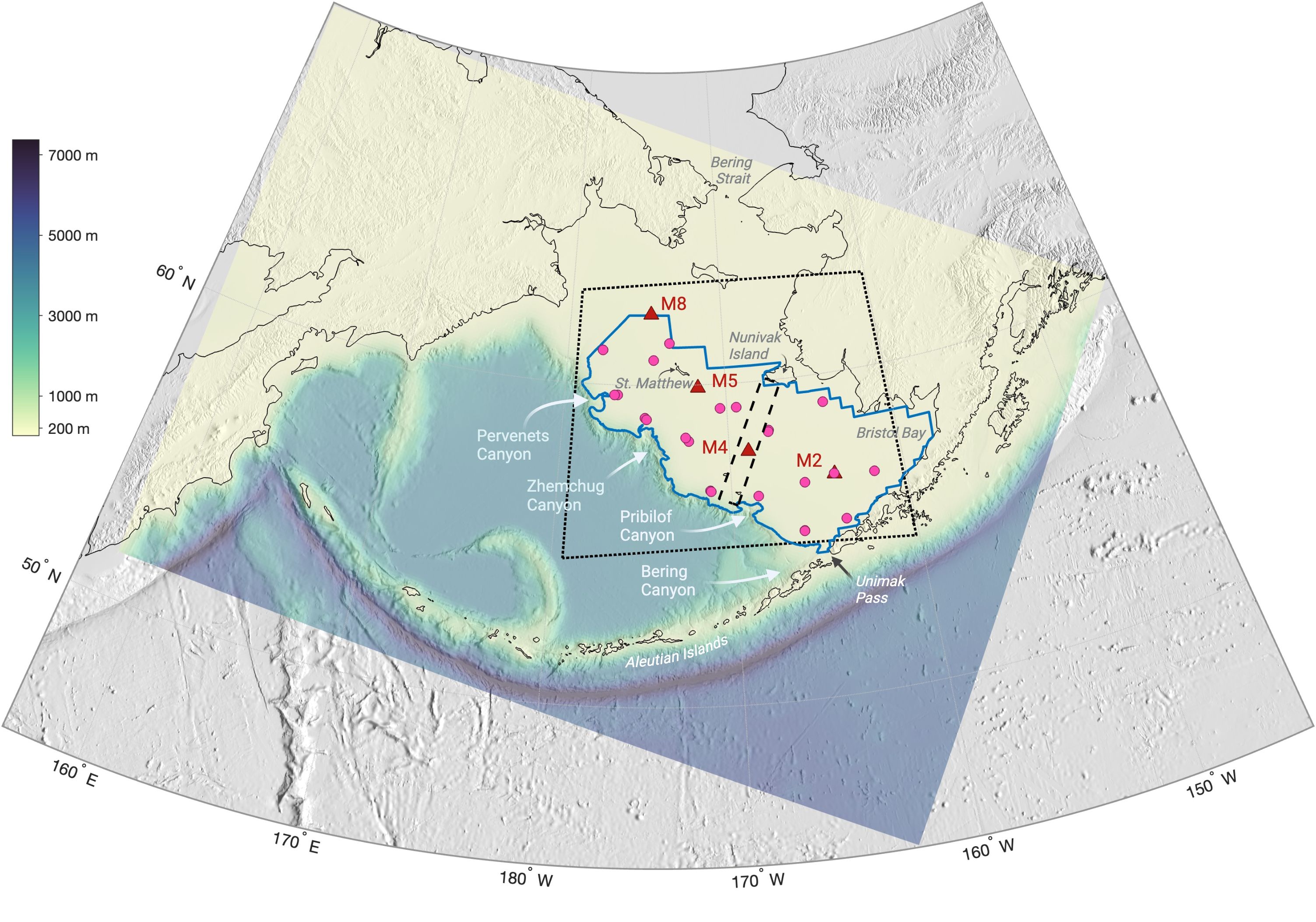
Figure 1. Map of the study area. The Bering Sea extends from the Aleutian Islands in the south to Bering Strait in the north. Shaded relief indicates bathymetry (ETOPO 2022 60 arc-second global relief model); bathymetry from the Bering10K model domain is overlaid in color. Pink circles indicate the pop-up float deployment locations, and red triangles show the locations of long-term moorings. The dotted black box highlights the focus area of this study (as seen in Figure 2), the blue line denotes the boundary of the groundfish survey sampling strata, and the dashed black box indicates the location of the transect in Figure 8. Key geographic features mentioned in the text are labeled.

This configuration, as described in detail in Kearney et al. (2020), reflects the setup of the “operational” hindcast that is updated twice annually and used to inform various management reports, such as the Bering Sea Ecosystem Status Report (Siddon, 2023). It has been demonstrated to capture key biophysical dynamics of the Bering Sea, including the seasonal extent of sea ice, formation of the cold pool, and general circulation and stratification patterns across the shelf Kearney et al. (2020); Hermann et al. (2013, 2016). For these experiments, the simulation was run from 1970–2023 in physics-only mode (i.e., coupled ocean and sea ice models but no ocean biogeochemistry) with daily mean archiving of the primary state and diagnostic variables.

2.2 Bottom temperature data sources

For this study, we compiled bottom temperature data for the southeastern Bering Sea shelf from a variety of sources. This included our newly collected pop-up float data as well as data from both long-term and project-based mooring deployments, an annual trawl survey of the shelf, and assorted CTD profile measurements. We briefly summarize the data collection methods for these data sources in the following sections.

2.2.1 Pop-up floats

Pop-up Floats are small (<35 kg in weight) monitoring instruments designed to be hand-deployed from a ship (Langis et al., 2018; Stabeno et al., 2020). PUFs have three modes of operation. In the first mode, the float remains anchored to the bottom for a preset time interval (6 to 12 months for this project) and records hourly data including bottom temperature. In the second mode, the float is released from the anchor at a prescribed time and records high-frequency data (∼4 Hz) during ascent through the water column. Once at the surface, the float transmits all data to shore and begins sampling in the third mode. This mode records hourly air and sea surface (0.5 m depth) temperature while onboard GPS provides precise location.

In the summer and fall of 2020, 13 PUFs were deployed through various partnerships including commercial fishing vessels, Pribilof Island residents, and the US Coast Guard. Unfortunately, it was realized in winter 2021 that the PUFs would have a problem sending data (this was confirmed when 11 of the PUFs surfaced in September 2021 as programmed but had problems reporting and only transmitted partial datasets.) We concluded that the stormy fall conditions when the PUFs surfaced, combined with inadequate freeboard, resulted in interference of the transmission antennas. Next-generation and more eco-friendly PUFs were developed using metal cans and an antenna and ballast design to fix the transmission problems that occurred in the earlier generation of PUFs. Nine of the next-generation PUFs were deployed during spring 2021 to supplement the earlier loss of data, and eight of these PUFs surfaced in September 2021 as planned. All eight successfully transmitted their full set of bottom temperature data. In fall 2021 and spring 2022, a total of 13 PUFs were deployed by the US Coast Guard and during research cruises. There were 10 successful data recoveries. In summary, 35 PUFs were deployed, with 26 surfacing, providing 4021 days worth of bottom temperature data, cumulatively. Bottom temperatures from the 26 successful data transmissions are included in Figure 2. PUF data was fairly evenly distributed across seasons, with 16.4%, 29.4%, 35.5%, and 18.8% of the total number of data points collected in climatological winter, spring, summer, and fall, respectively.

Figure 2

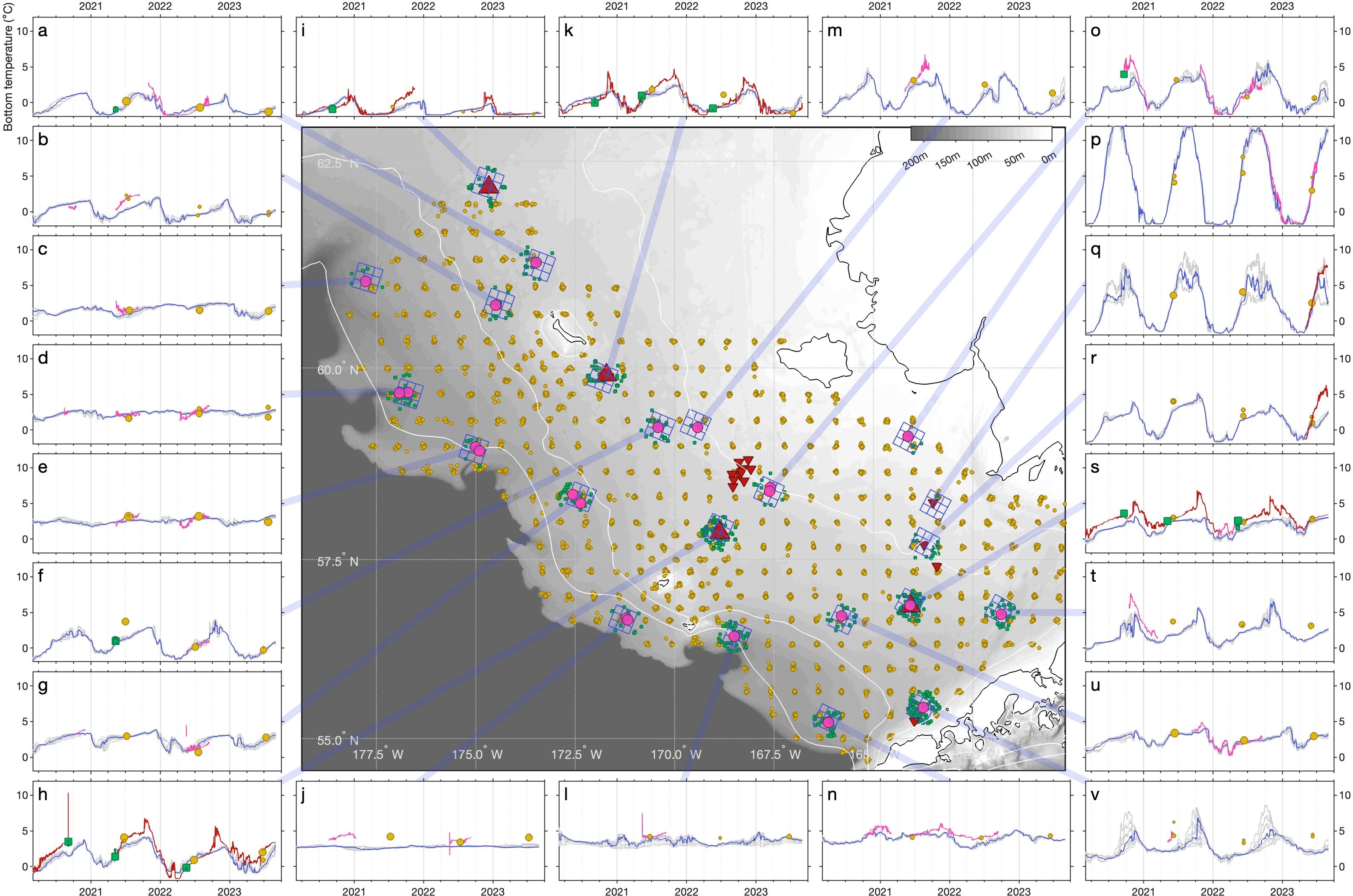
Figure 2. Center panel: Map of southeastern Bering Sea shelf bathymetry (grayscale shading, from ETOPO 2022) and location of various datasets: pink circles = pop-up floats, small gold circles = groundfish survey sampling locations, large red triangles = long-term moorings, small red inverted triangles = project-based moorings (Inner Front and Kuskokwim deployments), small green squares = CTDs. Blue grids show the location of the nearest Bering10K grid cell to each mooring/PUF cluster centroid and its 8-connected neighbor grid cells. White lines indicate the 50-, 100-, and 200-m isobaths in the Bering10K model configuration. Panels (A–V) show time series of data associated with those datasets for each cluster around the pop-up floats, long-term moorings, and Kuskokwim moorings for the period of June 2021–Aug 2023, using the same color scheme as in the center panel; for the model, the blue line indicates the center nearest-to-observation grid cell with gray lines for the remaining grid cells. Time series data points associated with CTDs and the groundfish survey data are scaled based on distance from the float or mooring location and includes any point within 26.2 km (i.e., the half diagonal length of the 20 nmi groundfish survey grid). Higher-resolution extended versions of the time series axes can be seen in Supplementary Figures S2–S23.

2.2.2 Groundfish survey

Bottom temperature data are collected during the Bering Sea bottom trawl survey. These surveys have been conducted by NOAA’s Alaska Fisheries Science Center annually since 1982 to assess the abundance, distribution, diets, and condition of commercially important groundfish and crab.

The primary survey region covers the southeastern Bering Sea shelf from Unimak Pass in the south to St. Matthew in the north, with survey stations distributed regularly on a 20 nmi grid (Figure 2 center, blue dots). The modern eastern Bering Sea (EBS) survey encompasses 376 sampling stations; the northern Bering Sea has also been sampled regularly since 2017, but we will focus on the EBS regions given the overlap with our focus area. The standard sampling plan uses two vessels to conduct the trawl surveys. Sampling begins with vessels on adjoining columns in the eastern end of Bristol Bay, and both vessels sample alternate columns moving westward across the shelf. The full survey takes approximately 2 to 4 months to complete each year, typically beginning in late May and concluding in mid-August. While the survey design attempts to maintain a consistent sampling order across years, the specific day of year when an individual station is sampled varies, with a per station standard deviation in sampling day-of-year of 6.7 days ± 1.5 days (mean and standard deviation across stations) and per station maximum range over the 40-year time series of 36.7 days ± 13.0 days.

Surface and bottom temperature data are collected during these surveys via bathythermograph. From 1982 to 1989, temperature data were collected via expendable bathythermographs (XBTs). More recent surveys use digital bathythermograph recorders attached to the headrope of the bottom trawl net (BRANCKER RBR XL-200 Micro BTs recorded at 6-second intervals for the 1993-2001 surveys, and a Sea-Bird SBE-39 bathythermograph continuous data recorder at 3-second intervals for 2002 to present). Temperature is then averaged over the on-bottom (∼2.5 m from bottom) and near-surface (∼5.5 m from surface) portions of the trawl (which covers a mean distance of 2.75 nmi) to produce a single surface and bottom (gear) temperature value per station per year. See Buckley et al. (2009) and Lauth et al. (2019) for further details of temperature data collection and post-processing.

2.2.3 Moorings on the eastern Bering Sea shelf

Long-term biophysical moorings have been maintained year-around at four sites on the eastern Bering Sea shelf (Figure 1). Moorings at M2 have been maintained almost continuously since 1995, M4 since 1999, and M5 and M8 since 2005. A full suite of biophysical data (temperature, salinity, chlorophyll fluorescence, currents, etc.) are collected at each site (see Stabeno et al. (2017) for details). These moorings are at the center of the seasonally-stratified middle shelf domain in water depths of 72 m to 74 m. Temperature, the primary data set presented in this manuscript, is collected at more than 10 depths at each mooring and within 8 m of the sea floor. The Bering Sea shelf waters are typically one- or two-layer systems, with tidal mixing leading to fairly uniform properties below the mixed layer (Kachel et al., 2002), so the deepest of these measurements is comparable to the bottom temperatures we use from the Bering10K model (bottom 5 m average) and trawl surveys (∼2.5 m from bottom).

We also use data from two major sets of moorings in the coastal domain (water depths <50 m). The first were deployed as part of the Inner Front Program (1997–99, Stabeno and Hunt, 2002) with the major array of moorings between Nunivak Island and the M4 mooring, positioned to assess the dynamics of a front that is nominally located along the 50 m isobath (Stabeno et al., 2016). The sharpness and specific location of the front varies from year to year dependent upon wind mixing, ice extent, and timing of the measurements (Kachel et al., 2002).

The second set of moorings were deployed in 2023 at three sites (water depth 25 m, 35 m and 50 m) on the inner shelf in the vicinity of Kuskokwim Bay. This was part of a program to explore the evolution of spring bottom temperatures in relation to demersal fish, and it included full water column moorings measuring temperature, salinity, and currents.

All instruments were calibrated prior to deployment and data were processed according to manufacturers’ specifications. Final processed temperature and salinity time series are accurate to at least ±0.002°C/m and ±0.0005 g/kg/m, respectively.

2.2.4 CTD profiles

NOAA hydrographic profile data collected in the Bering Sea, Chukchi Sea, and Gulf of Alaska over the past five decades – primarily under the Outer Continental Shelf Environmental Assessment Program (OSCEAP), Bering Arctic Subarctic Integrated Survey (BASIS), and Ecosystem and Fisheries Oceanography Coordinated Investigation (EcoFOCI) programs – has recently been compiled into a cohesive, quality-controlled dataset (Mordy et al., in prep.¹). This dataset includes CTD sampling from 1974–present and nutrient sampling from 2001–present. For this study, we used temperature data from version 0.97 of the top-250m CTD data product. We filtered for profiles 1) collected within the Bering Sea and 2) where the deepest temperature value corresponded to a pressure value (db) within 10 of the measured bottom depth (m). This filtering eliminated any partial water column profiles or profiles extending deeper than 250m. We then extracted the bottommost temperature value from each profile. In total, bottom temperature was extracted from 12191 profiles. While this data spans the entire shelf region and all ice-free seasons (i.e., outside of Nov–Jan), sampling is highly skewed toward a few well-sampled transect lines (see Supplementary Figure S1). As such, the spatiotemporal density of these measurements is too sparse to provide for quantitative validation of the model simulations, but we use these data as a qualitative check to enhance our understanding of seasonal and interannual variability at some of the more lightly-measured locations in our study. The 1713 of these specific CTDs used for this purpose are those located near our mooring/PUF analysis sites and are depicted in Figure 2 and Supplementary Figures S2–S23.

2.3 Baseline summer skill assessment

Given its broad spatial coverage and 42-year temporal coverage, the Bering Sea groundfish survey temperature dataset provides a means to spatially evaluate regional model skill in replicating summer bottom temperature. A preliminary skill assessment based on this data was previously conducted using 1982—2019 data (Kearney, 2021). Here, we repeat this skill assessment to incorporate data through 2023 and to bring our methodology in line with recently standardized methods to spatially interpolate survey-based temperature measurements across the southeastern Bering sea shelf (Rohan et al., 2022). As described in Section 2.2.2 above, one bottom temperature data point is collected at each of the 376 groundfish survey stations each summer. These data points are then interpolated to a 5-km resolution raster via ordinary kriging with a Stein’s Matérn semivariogram model. The interpolation allows for estimation of spatial structure of temperature patterns across the shelf and for more robust calculation of spatial metrics such as the cold pool index, i.e. fraction of the shelf with water below a certain threshold (usually -1°C, 0°C, 1°C, and 2°C) than a simple weighted average of the survey points themselves. The particular interpolation algorithm was selected from a pool of interpolation candidate methods based on its ability to reproduce spatial patterns even when data points were deliberately removed from the dataset (Rohan, 2022); this allows for more robust continuity across years even if occasional data points are missing. These interpolated rasters underlie a number of standardized survey-based temperature products produced by the Alaska Fisheries Science Center in support of their annual stock assessment activities.

We note that the spatially-resolved rasters do not reflect a static snapshot of Bering Sea bottom temperature. Rather, because data is collected over a period of 2–4 months, the spatial patterns reflect conditions at the time of sampling, with the southeasternmost portions (i.e., Bristol Bay) being more representative of early summer conditions and the northwesternmost parts reflecting late summer conditions. Therefore, to robustly assess the model’s skill, we choose to recreate similar model-derived non-synoptic rasters, rather than simply extracting a summer mean or similar from the model output. We do this by extracting a corresponding model-based dataset of bottom temperatures, with each point matching the nearest grid cell and daily time slice to each survey-based point. We then repeat the interpolation procedure to create a paired set of survey-derived and model-derived bottom temperature raster layers for each year in the 1982–2023 survey.

We assess model skill through a set of skill metrics, each applied to the 42-year time series at the raster grid cell level. These metrics were selected following Jolliff et al. (2009) and Stow et al. (2009) to quantify various aspects of model performance and are summarized in Table 1. The Bering Sea is a dynamic region, with high seasonal as well as interannual variability in bottom temperature. From an ecological perspective, it is important that the model properly capture the mean values, and in particular that it produce water below certain thresholds (e.g., 0°C and 2°C), since these appear to be critical thresholds for habitat preference or avoidance for key species. Skill in capturing year-to-year variability is equally important given that survival and recruitment dynamics for key fish species are tightly linked to warm/cold year oscillations (Hunt et al., 2011). We chose our skill metrics to reflect different aspects of the model’s ability to match both value and variability across the 40-year time series. Correlation can quantify covariability between the model and observations. In this annually-resolved analysis, a high correlation can indicate skill in capturing interannual variability, but may also be influenced by seasonal oscillations due to the non-synoptic nature of the observations (e.g., for a station sampled in early June one year and July the next, the correlation will quantify the model’s ability to capture the seasonal warming from June to July as well as any warming/cooling trend from one year to the next). Bias will reveal any systematic offsets in the mean value. Normalized standard deviation measures whether the scale of interannual variability matches that in observations, with values less than one indicating underestimated variability and vice versa. Model efficiency (MEF) summarizes whether the model is a better predictor of bottom temperature relative to a simple mean of the observations, highlighting skill in capturing both mean value and the specific variations in warm versus cold conditions that characterize this region; a value near one indicates high agreement between model and observations, while a value of zero indicates performance on par with a simple average of observations, and less than zero means the simple average provides a better prediction than the model.

Table 1

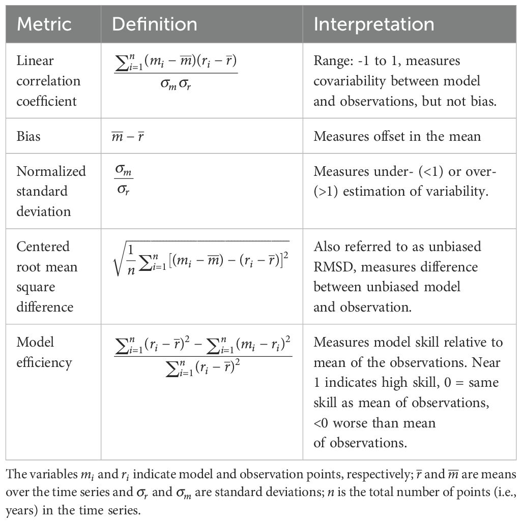
Table 1. Skill metrics used in this study.

3 Results and discussion

Maps depicting skill metrics relative to the 1982–2023 summer groundfish survey are depicted in Figure 3. The survey-based mean summer bottom temperature (Figure 3A) is characterized by the cold pool (<2°C) covering most of the middle shelf, with the coldest portions confined mostly to the northern half of this pool. The survey-based standard deviation (Figure 3B) is between 1.5 and 2°C across most of the inner and middle shelf, with slightly lower variability along the outer shelf. These values reflect the large interannual variability in bottom temperatures relative to the ∼4°C spread in mean values across the shelf.

Figure 3

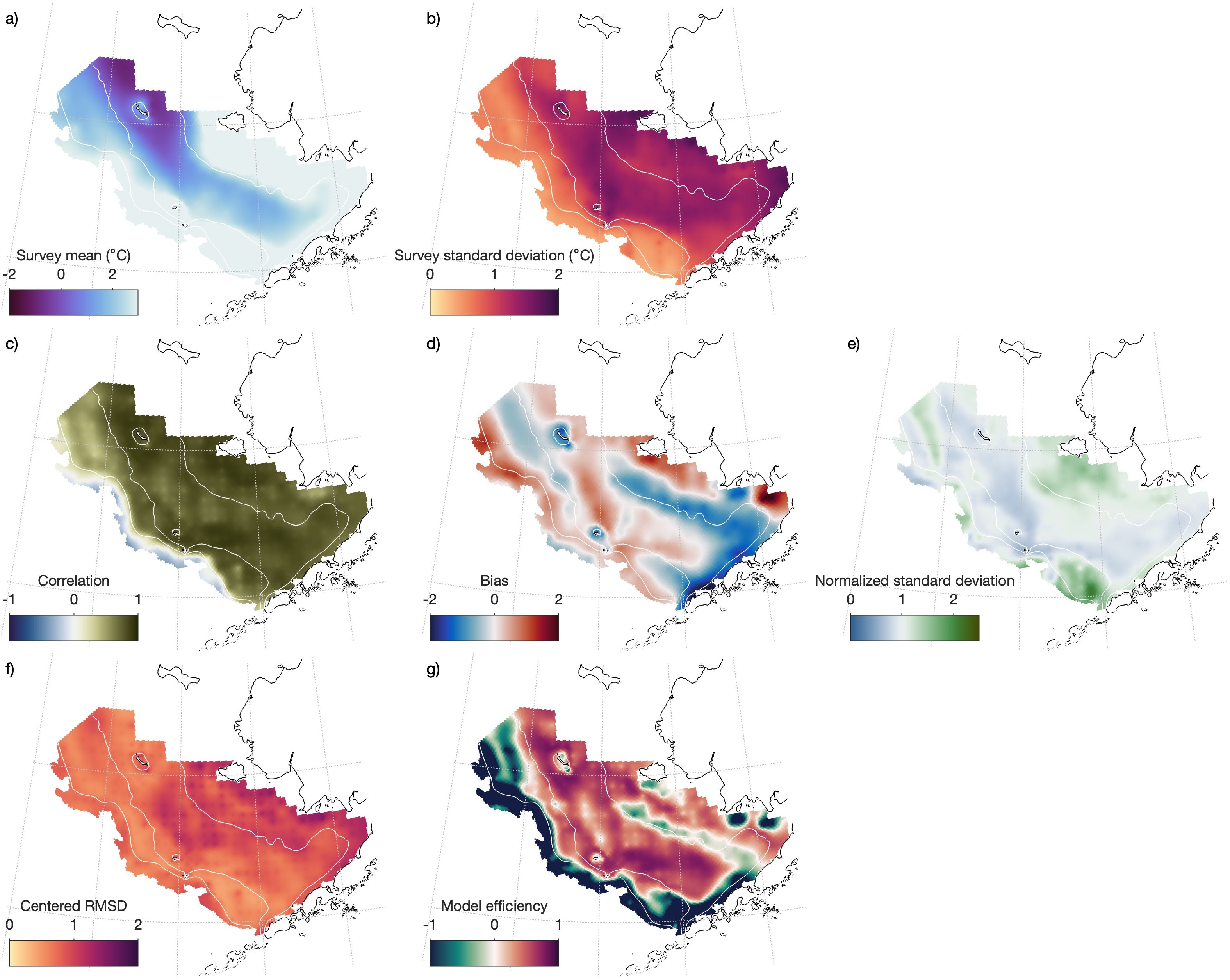
Figure 3. Skill statistics for the Bering10K survey-replicated rasters relative to the groundfish survey-based rasters. Panels (A, B) show the mean and standard deviation, respectively, of observation-based bottom temperature over time. The remaining panels depict skill of the model survey-replicated raster relative to the observational raster, including (C) correlation, (D) bias, (E) normalized standard deviation, (F) centered root mean squared difference, and (G) model efficiency. White contours indicate the 50 m, 100 m, and 200 m model isobaths.

Overall, our skill results suggest that the Bering10K model is able to capture the dominant bottom temperature patterns seen in the summer-only data across the southeastern Bering Sea shelf. Correlation is high across the vast majority of the shelf, with the exception of a strip along the shelf break and a region of slightly lower values in the northwest. Bias is spatially heterogeneous, but most (89%) of the shelf has an absolute bias of less than 1°C with a shelf-wide mean bias of only 0.06°C. Relative standard deviation is close to 1 across the shelf; interannual variability is overestimated in the inner shelf region and in the southwest near Bering Canyon, and slightly underestimated across most of the middle shelf. Model efficiency is well above zero for most of the shelf but less than zero (indicating underperformance relative to a simple average of observations) in a few key areas: the shelf break region, northwestern outer shelf, and regions along the inner front.

To look more closely at these patterns, we divide the shelf into a few sub-regions with shared skill metrics (Figure 4):

● Inner shelf: inshore region from the 50 m isobath, excluding waters in the immediate vicinity of the structural front that follows that isobath

● Middle shelf: between the 50 m and 100 m isobath, again excluding waters in the immediate vicinity of the structural front

● Inner front: region along the southern portion of the 50 m isobath with negative bias and model efficiency

● Shelf break: region between the 200 m isobaths as defined by real-world bathymetry vs the model grid bathymetry

● Northwest: northern portion of the outer shelf with negative model efficiency

● Alaska peninsula: southern portion of the shelf just north of the Alaska Pensinsula

Figure 4

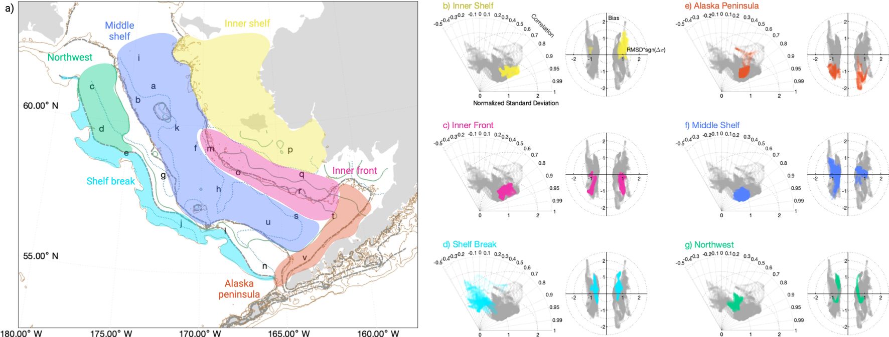
Figure 4. (A) Map of analysis regions as indicated by colored polygons: inner shelf = yellow, middle shelf = blue, shelf break = cyan, northwest = green, Alaska peninsula = orange, inner front = pink. Also depicted are the features used to define these regions: bathymetric contours for the model (dashed gray) and real world (thin brown), the 0-value contour from the bias (dashed blue), and 0-value contour of model efficiency (solid green). Letters correspond to the subpanel labels from Figure 2. (B–G) Taylor and target diagrams summarize the skill metrics for each raster grid cell by region. Taylor diagrams (left) depict the relationships between normalized standard deviation (radial axis), correlation (angular axis), and RMSD (dotted lines, distance from [1,1]); target diagrams (right) indicate the relationship between unbiased RMSD (x-axis), bias (y-axis), and total RMSD (dotted lines, distance from origin).

Skill metrics for raster grid points falling within each of these regions are depicted via Taylor and target summary diagrams in Figures 4B–G.

3.1 Inner shelf

The inner shelf domain of the southeastern Bering Sea shelf is typically defined as the portion of the shelf with less than 50 m bottom depth. This region is well-mixed year-round, which means bottom temperatures in this region are tightly coupled to surface forcing (Kachel et al., 2002; Mordy et al., 2017).

The summer skill metrics indicate that simulated bottom temperature in this region demonstrates high correlation (0.84 ± 0.23, mean and standard deviation across raster points) with the groundfish survey measurement. Interannual variability is higher in the model than in the observations (normalized standard deviation = 1.26 ± 0.16), and there is a bias of 0.51°C ± 0.35°C. Centered RMSD in this region is 1.05°C ± 0.13°C, the highest of the regions we analyze. A region just south of Nunivak Island shows negative model efficiency, but in the majority of the region the MEF remains high (0.32 ± 0.26).

Among the PUF suite, only one float (Figure 2P) was deployed within the inner shelf region and far from the structural front separating the middle and inner shelf domains (which we will address shortly). The comparison between the model and pop-up float data here show a very strong match across the nearly full-year time series, with the model capturing the large swings between summer temperatures over 10°C and winter temperatures at the near-freezing minimum of -1.7°C. As such, while the biases in this region appear larger relative to those seen in the rest of the domain, they are quite small relative to the seasonal amplitude of bottom temperatures in this area. In addition, the stations in this area are typically sampled in mid-June, which corresponds to a period of rapid warming. Because of this, the biases seen in this region may reflect small phenological mismatches, on the order of a few days, rather than biases in absolute value. Overall, the new PUF data suggests that the Bering10K model does capture the seasonal oscillations that dominate this region, lending increased confidence to the model output in this region.

3.2 Middle shelf

The middle shelf domain is typically defined as the region between 50 m and 100 m depth and is characterized by strong seasonal stratification. Summer bottom temperature values experience high interannual variability associated with variations in the extent of sea ice across the shelf (Coachman, 1986; Sambrotto et al., 1986; Stabeno et al., 2012). The seasonal amplitude of variation also varies around 5°C, with lows in the winter months and highs in late fall following destratification of the water column. This region is the most well-studied portion of the shelf, with data regularly collected on cruises along the 70-m isobath, along with the presence of several long-term moored buoys. In addition to those moored buoys (from north to south, Figures 2H, I, K, S), PUFs were deployed throughout this region (Figures 2A, B, F, S, U).

Collectively, the time series from this domain reaffirmed the model’s ability to capture summer bottom temperatures in both the northern and southern portions of the middle shelf. MEF is 0.54 ± 0.17, the highest of all regions; and bias and RMSD are the lowest across regions at 0.09°C ± 0.35°C and 0.84°C ± 0.20°C, respectively. This skill appears to extend into the winter and spring months as well, when bottom temperature is tightly coupled to sea ice. In particular, at the location of the PUF depicted in Figure 2U, the model was able to capture small oscillations in 2022 winter bottom temperature associated with short advances and retreats of the sea ice edge.

However, the majority of the time series in this region also reveal mismatches between the model and mooring time series in the late summer and early fall months. In many cases, the observations indicate a steady increase in bottom temperature during this time, often with a sharp peak in fall. The model consistently underestimates this warming and shows an absence of the fall peaks. By examining surface and bottom temperatures measured at the middle shelf moorings alongside each other, we can see that these peaks correspond to periods of destratification, when the water column mixes vertically, bringing heat from surface waters to depth (Figure 5). While the model closely tracks both surface and bottom temperature at these locations for much of the year, it does not appear to show the same amount of warming in late summer, and destratification is typically delayed. We estimated destratification date as the first post-ice-season day of year when surface and bottom temperatures were less than 0.2°C apart for at least 20 consecutive days (Figure 5, triangles). By this metric, the model remains stratified for a mean of 18, 21, 34, and 44 days longer than the mooring at the M8, M5, M4, and M2 mooring locations, respectively. Because surface temperatures are lower at the later date, the simulated destratification process does not transfer as much heat to the bottom layers, resulting in a lack of the small peaks seen in the observational time series. The lack of deep mixing in the fall reflects a known and recalcitrant problem in the commonly-used K profile parameterization surface boundary layer scheme when attempting to represent the full suite of processes that contribute to surface mixing in subpolar regions (Damerell et al., 2020). The Bering10K model specifically tends to underestimate mixed layer depth year round when compared to CTD and mooring-based measurements (Hermann et al., 2013, 2016; Kearney et al., 2020). As a result, heat from surface fluxes tends to be confined to a too thin surface mixed layer, leading to small positive biases in sea surface temperature and negative biases at depth. The time series data suggest that this underestimation of deep mixing is particularly problematic when simulating the timing of and heat redistribution associated with fall destratification on the middle shelf.

Figure 5

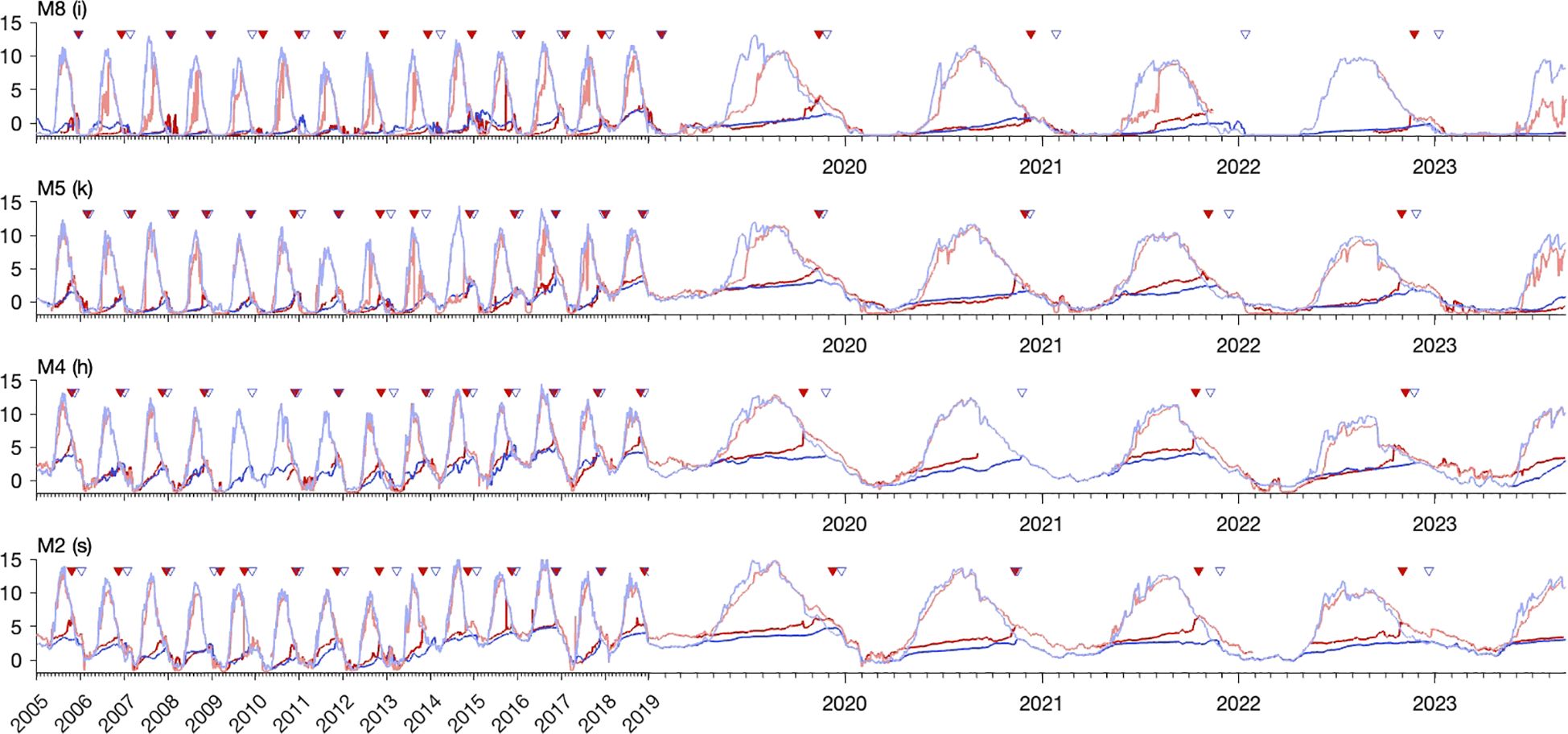
Figure 5. Surface (light) and bottom (dark) temperatures at long-term mooring sites (red) and in the Bering10K model (blue). Triangles near the top of each axis indicate destratification events in the mooring (solid red) and model (open blue), defined as the first time in the fall of each year when surface and bottom temperature differ by less than 0.2°C. Axis arrangement corresponds to latitude of the mooring sites, with M8 farthest north and M2 farthest south; letters in parentheses match the corresponding subpanels in Figure 2.

While this study focuses on bottom temperature, we also note the occasional larger mismatches in surface temperature observed at the moorings in early spring, particularly at the northernmost mooring (M8) in this study, as seen in Figure 5. The rise in surface temperature at this location is expected to coincide with the retreat of sea ice, once the water column is exposed to atmospheric heat fluxes. This model has previously been shown to have a small systematic late bias of approximately 2 weeks in its date of sea ice retreat when assessed against satellite-based datasets (Kearney et al., 2020). However, the mismatches highlighted here show an opposite directionality, i.e. model surface warming precedes observations. While the simulated surface temperature rises steeply once modeled fractional ice coverage is below 0.1, the mooring surface temperatures increase much more gradually when observed ice (as measured by satellite) reaches the same thresholds, with the steeper increase lagging ice retreat by 1-3 months (Supplementary Figure S24). We hypothesize that this mismatch may be due to the measurement depth of the M8 mooring’s surface sensor. To avoid damage from ice, the surface-most sensor on this mooring is at 14 m depth. Therefore, the “surface” measurements here may not capture true surface values, particularly when freshwater from ice melt leads to stratification in the near surface waters. A more accurate analysis of model SST skill relative to the mooring would need to compare values from this subsurface depth rather than the top 5m average used in this particular figure. However, this mismatch in surface warming does not impact our analysis of bottom temperature.

3.3 Shelf break, northwest, and Alaska Peninsula

The shelf break region, defined here as regions offshore of the model’s 200 m isobath but inshore of the real-world 200 m isobath, stands out from the rest of the shelf in terms of poor model performance (Figures 3, 4D). Model efficiency is less than zero throughout this region (-2.18 ± 1.28), and correlation is near zero and even negative across much of it (0.04 ± 0.20). This poor performance stems from limitations in the Bering10K model’s representation of the continental slope. Sigma-coordinate models such as ROMS are subject to computational errors in the horizontal pressure gradient along regions where topography is steep or the vertical gradient in a property is large (Shchepetkin, 2003); this limitation often necessitates applying a smoothing filter to the bathymetry, as was done for the Bering10K domain and its predecessor northeast Pacific (NEP) domains (Danielson et al., 2011; Kearney et al., 2020). The smoothing process decreases the steepness of the shelf break by applying a modified Shapiro filter to the depth values in regions of high steepness, resulting in a slope region with a wider horizontal footprint than in the real world and thus a simulated shelf that is slightly narrower than the real-word one (Figure 6). Topographical features along the shelf break, such as canyons, are also less fully resolved as a result of the smoothing filter.

Figure 6

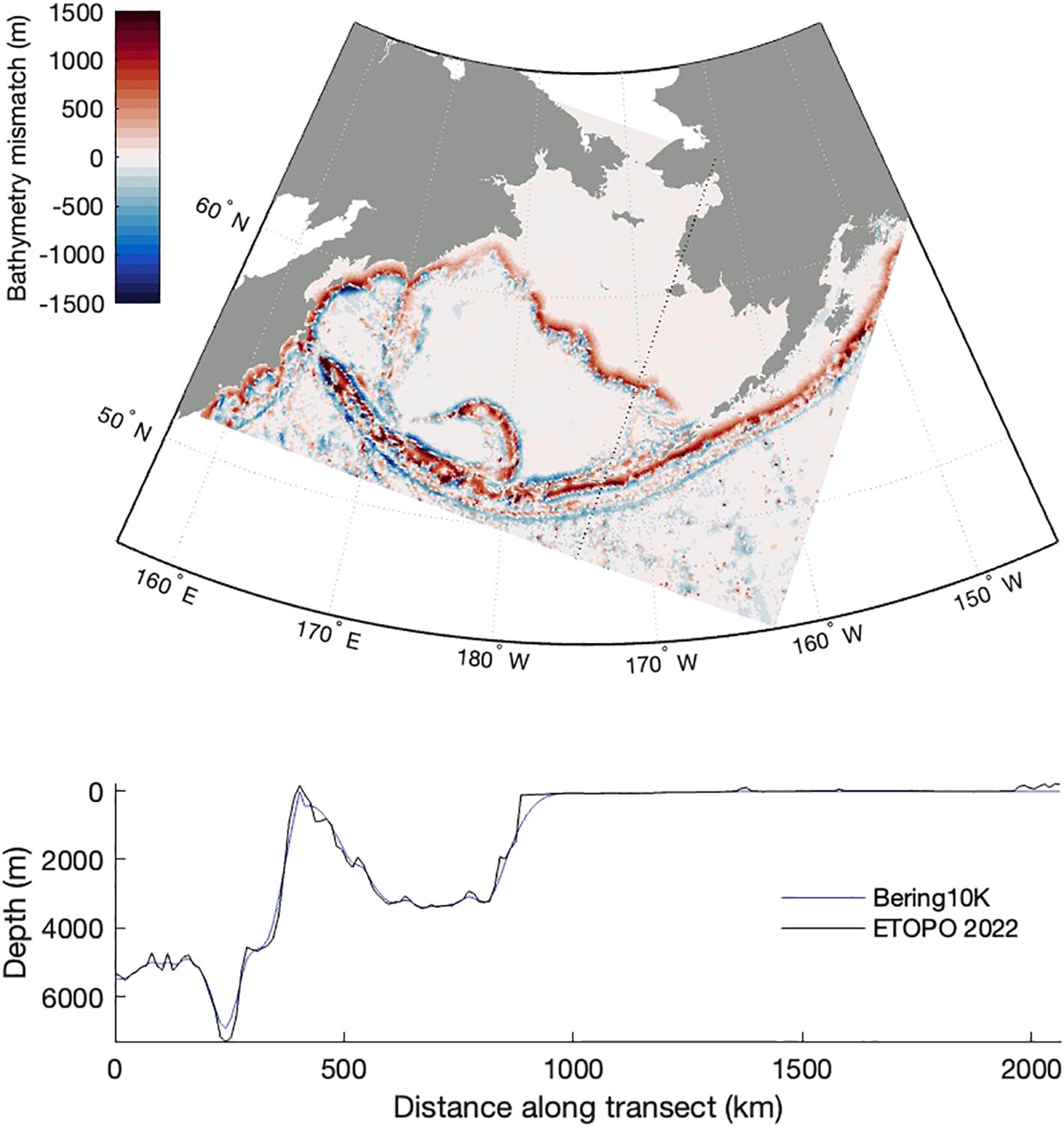
Figure 6. Mismatch between the Bering10K grid bathymetry and ETOPO 2022 bathymetry (positive values indicate model is deeper than ETOPO 2022). The bottom panel depicts bathymetry along the dotted black transect line extending from the Gulf of Alaska at 0 km, across the Aleutian trench and Aleutian Islands, into the Bering Sea basin, and onto the eastern Bering Sea shelf.

This bathymetric smoothing leads to two separate issues. The first, reflected in the skill statistics along this shelf break area, is that our assessment methodology compares two fundamentally different things in the shelf break area itself: real-world observations collected in outer shelf waters with depths of just under 200 m, and simulated data collected on the continental slope or in the basin with water depths of 1000 m or more. This can be seen in the PUF deployments in Figure 2J (and Supplementary Figure S11). While the float deployments at this location were short, they show indications of seasonal warming from spring into fall; groundfish trawl measurements indicate modest interannual variability reflecting shelf-wide warm and cold periods. However, the model shows bottom waters that remain stable over time, with little indication of seasonal or interannual cycles, which is typical for bottom waters in the deep basin (in both the model and in observations) that are well below the mixed layer year-round and thus isolated from surface heating. This problem, which is unavoidable in sigma-coordinate models, poses difficulties when using such a model in a living marine resource context. Physical processes along the shelf break induce high mixing that bring macronutrients from depth and micronutrients like iron from the shelf, supporting high primary productivity (Ladd, 2014; Stabeno et al., 2016). So while the shelf break occupies a small statistical percentage of the overall model domain, that region is often one that plays an outsized ecological role as preferred habitat for key species.

The bathymetric smoothing can also contribute to decreased skill in regions further from the depth mismatch region itself due to its impact on circulation features. The eastern Bering Sea slope is incised by several large submarine canyons, which interrupt the flow of the Bering Slope Current that flows northward and can act to increase the flow of basin water onto the shelf (Sigler et al., 2015). The canyons are less sharply resolved in the Bering10K model, and as a result, regions that are influenced by this on-shelf transport show decreased correlation and model efficiency metrics. This includes the southern regions along the Alaska Peninsula, where flow from the basin through Bering Canyon and from the Gulf of Alaska through narrow passes in the Aleutian Islands contribute to the bottom temperature patterns. This region shows the strongest negative bias in the domain (-1.18°C ± 0.35°C). The pop-up floats deployed in this region (Figures 2T, V) also suggest that the cool bias is present throughout the year. A cool bias in this region would be consistent with an underestimated flux of relatively warm basin water from off shelf regions. The lack of flow through canyons also impacts the northwestern portion of the shelf, where flow through Zhemchug Canyon may be an important contributor to bottom temperature. The pop-up floats deployed in this northwest region cover only partial years (Figures 2C, D), but hint at higher seasonal variability in this region than is seen in the model.

We can confirm the lack of preferential transport through these canyons by running some simple offline reverse particle tracking using the daily-averaged Bering10K output (Figure 7). We calculated the reverse trajectories for passive particles released in these two regions using the ROMSPath three-dimensional offline particle tracking package (Hunter et al., 2022). 800 particles were released, in clusters of 20 points each randomly positioned within a 20-nautical mile box around manually-chosen groundfish survey stations within the regions of interest (to ensure approximately even spatial distribution across the regions), for a total of 320 particles in the Alaska Peninsula region and 480 particles in the northwest region. All particles were initiated at a depth 5 m above the bottom. Trajectories were then simulated using reversed-sign velocities from the Bering10K output starting on July 6, 2021 12:00 (chosen as the archived time step closest to a “mid-summer” July 1 date in a year with conditions near the long-term interannual mean) and extending backwards for 365 days. While this simple offline simulation does not account for sub-daily velocities within the fully-resolved Bering10K simulation, particularly tidal velocities, and therefore may underestimate variability in particle trajectories, it provides a rough estimate of where summer bottom water in each region originates in this model. In the Alaska peninsula region, a small portion of the particles entered the region from the Alaska Coastal Current that runs along the northern Gulf of Alaska and then enters the Bering Sea through Unimak Pass. The majority of the particles, though, originated in the nearby shelf regions along the Bering Sea side of the peninsula and in Bristol Bay. No particles crossed the shelf break in the vicinity of Bering Canyon, indicating the possible missing on-shelf flow in this region in the model. The northwest region showed similar high retention times, with many particles showing very little net movement over the one-year simulation. Some particles did move onto the shelf from the Bering Slope Current, which runs northward along the shelf break (this includes particles that originated near the western shelf; those trajectories crossed onto the shelf after merging with the Bering Slope Current and moving in a northward direction). However, the trajectories of these particles moved onto the shelf at various places, with no clear funneling of particles in the vicinity of Zhemchug or Pervenets canyons. This particle-tracking exercise suggests that the poorly-resolved geometry of the shelf break and the Aleutian passes may at least in part contribute to the biases in these two regions. However, we also note that flow in and around these canyons is not well-constrained by observations, with much of our present understanding inferred from observations of mesoscale eddies along the shelf break (Schumacher and Stabeno, 1994; Mizobata and Saitoh, 2004). Therefore, this region warrants further inquiry to better understand the processes transporting water across the shelf break, whether regional models are appropriately representing those processes, and whether our bathymetry-smoothing hypothesis fully explains the low skill metrics in these portions of the shelf.

Figure 7

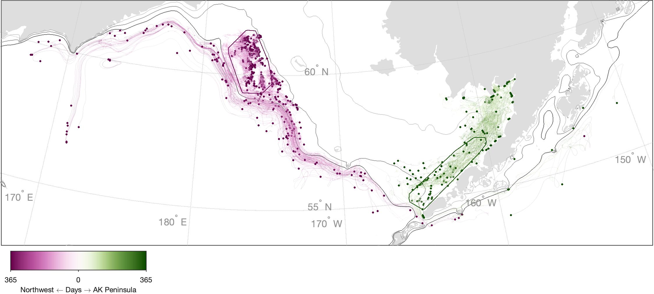
Figure 7. Reverse particle tracks for particles released in the northwest (purple) and Alaska Peninsula (green) regions. Polygons indicate the convex hull of the release points for the particles, colored lines indicate the trajectory of the reverse tracks for one year, and dots indicate the final (origination) location of the trajectory after a 366-day simulation. Gray contours indicate the 50 (light), 100 (medium), and 200 m (dark) isobaths of the Bering10K model.

3.4 Inner front

In the summer, the unstratified inner domain and thermally-stratified middle domain are separated by a structural tidal front. This front is typically located along the 50 m isobath, although its exact location varies from year to year. The existence of this front is well-established by numerous ship- and mooring-based measurements (Coachman, 1986; Stabeno et al., 2001; Kachel et al., 2002). The front is a highly dynamic feature, with its exact location varying based on wind and tidal mixing (Kachel et al., 2002; Mordy et al., 2017).

In our skill assessment, this region is characterized by a low (and sometimes negative) MEF values (0.21 ± 0.30) and a cool temperature bias (-0.61°C ± 0.33°C). It has been previously hypothesized that these low skill metrics may indicate a nearshore spatial bias in the model’s positioning of the inner front. However, the real-world front is primarily a subsurface feature, and as such the limited number of measurements of the front location are not sufficiently resolved in space and time to allow a quantitative assessment of the proposed spatial mismatch. Using the additional seasonal data provided by the mooring and PUF data, we explored two potential hypotheses for why these low skill values manifest in this region.

First, the low skill metrics, particularly the MEF, may simply reflect the challenge of perfectly simulating the exact location of the front, given its dynamic spatiotemporal variability, rather than a systematic offset. Waters on the nearshore side reflect the strong summer warming signal of the inner domain while middle domain bottom waters remain cold until the fall. As a result, a very small offset in simulated location of the front can lead to a disproportionate mismatch in value. This can be seen, for example, in Figure 2Q, where the mooring was deployed immediately adjacent to the simulated front in 2023. The closest model grid cell (indicated by the blue line) shows a discrepancy between the mooring and model data of nearly 3°C by the late summer. However, an immediately adjacent grid cell tracks that mooring time series nearly perfectly. Similarly, historical groundfish survey temperature values at other locations along this front (Supplementary Figures S14, S16, S19) often fall within the spread of values indicated by the 8-nearest-neighbor model grid cells even if they do not match the nearest one. Sampling along this region typically takes place very near to the onset of stratification, so very small offsets in both the spatial location and timing of front formation can lead to low skill metrics despite relatively skillful simulation of the dynamics on either side of the front.

Given the consistent negative bias in this region, though, we don’t believe the low skill metrics can be entirely attributed to these small spatiotemporal variations. The cool bias instead suggests the model stratification either persists longer in time or reaches farther inshore than in the real world. Temperature profiles measured during the 1995–1999 inner front study were examined to test this hypothesis. We analyzed model data from model grid cells η=89, ξ=80–120 (where η and ξ are the along-shelf and cross-shelf axes of the model grid), a transect that passes adjacent to the primary mooring deployment location (Figure 8A). We then estimated stratification in both the model and the mooring profiles using an index of the potential energy required to mix the water column, after Simpson et al. (1977):

Figure 8

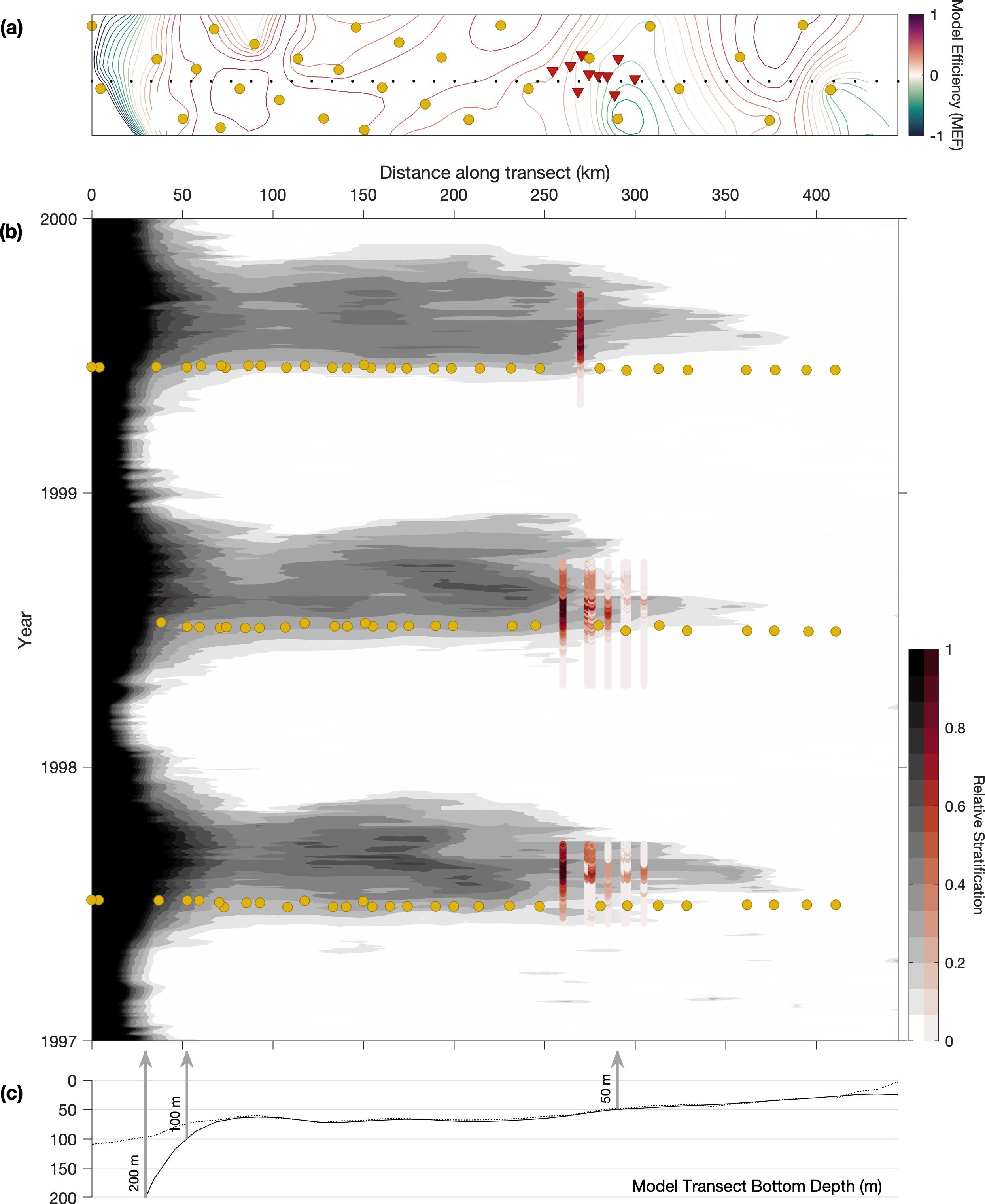
Figure 8. (A) Map of mooring deployments (red triangles) and groundfish survey stations (gold circles) near the transect of model grid cells (black dots). The horizontal axis is oriented along the transect line and the vertical axis is orthogonal to the transect; the location of this transect box is depicted in Figure 1 by the dashed black line. Contours of the model efficiency metric (identical to the data in Figure 3G) are shown by colored lines. (B) Model-based relative stratification index (grayscale) is plotted across time (vertical axis) and distance along the transect (horizontal axis). Daily-averaged relative stratification index values based on the inner front mooring profiles are overlaid using the red colorscale at the corresponding location and time of each measurement. Groundfish survey sampling points (gold circles) are also added to indicate where sampling near this transect occurs in time and space. (C) Bering10K bottom depth (solid black line) along the transect line, with arrows indicating the location of the 50 m, 100 m, and 200m isobaths along this transect. Bathymetry from ETOPO 2022 (dotted black line) is also shown for reference.

$\begin{array}{ll}SI=\frac{1}{\zeta +h}{\int }_{-h}^{\zeta }g(\zeta -z)(\rho -\overline{\rho })dz& (1)\end{array}$

$\begin{array}{ll}\overline{\rho }=\frac{1}{\zeta +h}{\int }_{-h}^{\zeta }\rho dz& (2)\end{array}$

where ρ is density, h is the depth of the water column, ζ is the height of the free surface, g is gravitational acceleration, and z is depth relative to mean surface height (i.e. ζ = 0). The vertical resolution of the two datasets is different, the values are not quantitatively comparable, making it difficult to compare the strength of stratification between model to mooring (the limited number of mooring depths were positioned to try to capture as much of the transition across the mixed layer as possible, but did not always fully capture surface values, leading to underestimations of stratification by this particular definition). However, the values can be qualitatively compared in a more binary sense (using SI>0 as an indication of stratification) to analyze the timing of stratification and destratification in each (Figure 8B), relative to each other and to the expected front location near the 50-m isobath (Figure 8C). This comparison shows that the model appears to be capturing the timing of stratification reasonably well, and also reflects the potential problems with delayed destratification in the fall. The inner-most moorings deployed in 1997 and 1998 show little to no stratification throughout their deployment, suggesting that these were deployed shoreward of the front location. However, for short periods of the early summer, the model-based stratification index suggests the modeled front extended almost 100 km farther inshore from the mooring location. This spatial offset could account for the cool bias and low model efficiency seen in the vicinity of the mean front location. We note that many of the groundfish survey points located within this region of model/data disagreement on front location are sampled early in the survey, so the high skill metrics associated with some of these locations neither supports nor refutes the model’s front location.

Overall, this analysis suggests that the model captures most of the key dynamics associated with formation of the inner front. However, the model appears to have a small spatial bias in the exact location of the front, and small temporal mismatches in front formation can lead to outsized mismatches in model/data bottom temperature due to the wide swings in temperature associated with destratification. These issues should not be problematic when focusing on the shelf as a whole but ecologists focusing on this frontal region in particular should be aware of potential limitations in capturing the dynamic nature of this region.

4 Conclusions

Regional ocean modeling is playing an increasing role in management activities in the Bering Sea, and as such, thorough skill analysis of the regional models in the biological context that they are being used is increasingly important. This paper assesses the key variable of bottom temperature as simulated by the Bering10K ROMS model against a number of different observational datasets with differing spatial and temporal coverage and resolution.

Overall, our skill assessment confirmed that the Bering10K model captures summer values very well across the majority of the shelf in terms of both climatological mean values and interannual variability. This remains an important benchmark for model skill in the Bering Sea since summer bottom temperature metrics are the most commonly-used indicators of ecosystem function across the Bering Sea shelf. While observational sampling is still skewed heavily in favor of summer data, year-round datasets from the pop-up floats and moorings suggest that the model likewise captures the cooling and stratification processes that control much of the seasonal evolution of bottom temperatures year round. This is particularly true across the inner and middle shelf regions. This validation lends further credence to ecological applications that rely on model derived bottom temperature across seasons, such as the investigation into Pacific cod thermal spawning habitat that motivated the pop-up float deployment (Bigman et al., 2023).

However, the analysis also highlighted a few key places where the model and observations diverged. The model tends to underestimate surface mixing, leading to a shallow bias in mixed layer depths across the domain (Hermann et al., 2016; Kearney et al., 2020). The mooring and PUF data suggest that this also leads to delayed destratification of the water column across the middle and outer shelves in the late summer and early fall. While this bias does not strongly impact estimates of bottom temperature during the summer, its impact is apparent when looking at bottom temperatures across the middle shelf region in the fall. It also leads to an underestimate of heat transport to depth associated with the destratification process. This bias may be important to consider when assessing temperature-related habitat that is strongly tied to specific temperatures during these late summer or early fall months, or to phenological aspects of the destratification process.

The analysis also suggests there may be a small bias in the positioning of the inner front, with the model placing it a bit closer to shore than real-world observations suggest it should be. However, observations of stratification along the front are sparse, and it is difficult to fully characterize the real-world position and variability of this feature. In general, the model captures the primary dynamics of front formation, but biologists should be aware of potential small spatial and phenological offsets in the exact location when using model data along this frontal region.

Finally, we note several regions of reduced skill linked to poor representation of steep vertical gradients along the shelf break within the model. This model limitation, which is imposed by constraints of the numerical integration scheme used in sigma-coordinate models like ROMS, was previously known to impact grid cells in the immediate vicinity of the overly-smoothed bathymetry. This current analysis reveals that it may also have further-reaching impacts due to under-representation of flow from the basin onto the shelf through slope canyons, especially Bering Canyon in the southwest and Zhemchug Canyon in the northwest. The northwest region in particular is not often a focus of Bering Sea research, and unfortunately many of the pop-up floats deployed in this region returned only partial time series. We highlight this region as one where future research should be directed to provide a better understanding of the key processes that regional models would need to capture to properly simulate habitat in this region.

The analyses in this paper present a general framework for validating model-simulated bottom temperature across the Bering Sea shelf. Under the Climate Ecosystem Fisheries Initiative, NOAA is currently pursuing a cohesive, cross-regional approach to developing and using regional ocean models in a management context. This program focuses on the development of the Geophysical Fluid Dynamic Laboratory’s Modular Ocean Model version 6 (MOM6) (Adcroft et al., 2019) for regional-scale applications, with successful development and deployment thus far of a northeast Atlantic domain (Ross et al., 2023) and ongoing development for northeast Pacific (Drenkard et al., 2024) and pan-Arctic domains. The MOM6 model offers several capabilities that may help alleviate some of the skill deficiencies noted in this paper. In particular, it allows for a hybrid vertical coordinate system that eliminates the need for bottom topography smoothing. Preliminary simulations of the northeast Pacific MOM6 model suggest significant improvement of biases along the Alaska Peninsula region relative to the Bering10K ROMS model that may be attributable to the MOM6 model’s more realistic shelf geometry (Drenkard et al., 2024). In addition, the MOM6 model’s use of the Bodner et al. (2023) mixed layer eddy parameterization with variable-scale frontal widths has shown promise in better capturing mixed layer depths and deep mixing processes in the subarctic regions of the domain (Drenkard et al., 2024). The analysis framework for this paper, including the source code to extract model output, compare to observations, and generate the figures for this paper has been written with the transition from the Bering10K ROMS model to the northeast Pacific MOM6 model in mind. As such, this in-depth skill assessment of bottom temperature offers a baseline that can be easily repeated to quantitatively assess and compare skill across future ROMS and MOM6-derived model output for the Bering Sea shelf region.

Data availability statement

The analysis code to reproduce the calculations and figures in this paper is available on GitHub at https://github.com/kakearney/PUFB10K_manuscript_supporting_code. This repository also hosts copies of the mooring and pop-up float data as used in this study. These data copies are preliminary and intended for reproducibility only. - CTD Dataset: Advance access to the CTD data associated with the Mordy et al. (in prep.) hydrographic compendium was received from Noel Pelland. This dataset will be uploaded to a public archive alongside the imminent submission of Mordy et al. (in prep.) for publication. This will be linked to the above GitHub site when it becomes available. - Bering10K ROMS model: Source code for the Bering10K ROMS model implementation is available on GitHub at https://github.com/beringnpz/roms-bering-sea. The specific implementation used in this study was compiled from the master branch, commit c5c726e, with physics-only options (see buildbering.sh in the repository); a snapshot of the source code is also archived through Zenodo under DOI 10.5281/zenodo.3376313. Selected output variables from the Bering10K daily-archived hindcast simulation, including the bottom temperature values used in this paper, are hosted on the Alaska Climate Integrated Modeling Project THREDDS Data Server at https://data.pmel.noaa.gov/aclim/thredds/catalog/files/B10K-K20nobio_CORECFS_daily.html. - Groundfish trawl survey: Temperature data from the surveys conducted under NOAA/AFSC/RACE’s Groundfish Assessment Program are archived through the coldpool R package, available on GitHub at https://github.com/afsc-gap-products/coldpool..

Author contributions

KK: Conceptualization, Formal Analysis, Investigation, Methodology, Validation, Visualization, Writing – original draft, Writing – review & editing. PS: Data curation, Funding acquisition, Writing – review & editing. AH: Data curation, Writing – review & editing. CM: Data curation, Funding acquisition, Writing – review & editing.

Funding

The author(s) declare that financial support was received for the research, authorship, and/or publication of this article. This research was funded by the North Pacific Research Board (NPRB) under Project #2003.

Acknowledgments

We thank all those who have contributed to the numerous field measurements we used in this study, and to those who contributed to previous ROMS model development in the Bering Sea. In particular, we thank Noel Pelland for providing access to and interpreting the EcoFOCI CTD dataset, and Shaun Bell for providing access to and formatting the long-term mooring datasets used in this study. Finally, we thank our two reviewers for their time, effort, and insights, leading to a more thorough and improved manuscript.

Conflict of interest

The authors declare that the research was conducted in the absence of any commercial or financial relationships that could be construed as a potential conflict of interest.

The author(s) declared that they were an editorial board member of Frontiers, at the time of submission. This had no impact on the peer review process and the final decision.

Publisher’s note

All claims expressed in this article are solely those of the authors and do not necessarily represent those of their affiliated organizations, or those of the publisher, the editors and the reviewers. Any product that may be evaluated in this article, or claim that may be made by its manufacturer, is not guaranteed or endorsed by the publisher.

Supplementary material

The Supplementary Material for this article can be found online at: https://www.frontiersin.org/articles/10.3389/fmars.2025.1483945/full#supplementary-material

Supplementary Figure 1 | CTD sampling density in space (left) and time (right).

Supplementary Figure 2 | Extended version (1985–2024) of time series data shown in Figure 2. For the model, the blue line indicates the center nearest-to-observation grid cell with light gray lines for the remaining grid cells. Observed data is depicted as follows: pink lines = pop-up floats, gold circles = groundfish survey, red lines = long-term moorings or project-based moorings, green squares = CTDs. Data points associated with CTDs and the groundfish survey data are scaled based on distance between the central model grid cell and the float or mooring location and includes any point within 26.2 km (i.e., the half diagonal length of the 20 nmi groundfish survey grid).

Supplementary Figure 3 | See Supplementary Figure S2 for details.

Supplementary Figure 4 | See Supplementary Figure S2 for details.

Supplementary Figure 5 | See Supplementary Figure S2 for details.

Supplementary Figure 6 | See Supplementary Figure S2 for details.

Supplementary Figure 7 | See Supplementary Figure S2 for details.

Supplementary Figure 8 | See Supplementary Figure S2 for details.

Supplementary Figure 9 | See Supplementary Figure S2 for details.

Supplementary Figure 10 | See Supplementary Figure S2 for details.

Supplementary Figure 11 | See Supplementary Figure S2 for details.

Supplementary Figure 12 | See Supplementary Figure S2 for details.

Supplementary Figure 13 | See Supplementary Figure S2 for details.

Supplementary Figure 14 | See Supplementary Figure S2 for details.

Supplementary Figure 15 | See Supplementary Figure S2 for details.

Supplementary Figure 16 | See Supplementary Figure S2 for details.

Supplementary Figure 17 | See Supplementary Figure S2 for details.

Supplementary Figure 18 | See Supplementary Figure S2 for details.

Supplementary Figure 19 | See Supplementary Figure S2 for details.

Supplementary Figure 20 | See Supplementary Figure S2 for details.

Supplementary Figure 21 | See Supplementary Figure S2 for details.

Supplementary Figure 22 | See Supplementary Figure S2 for details.

Supplementary Figure 23 | See Supplementary Figure S2 for details.

Supplementary Figure 24 | SST and fractional sea ice cover in the Bering10K model (blue) are closely coupled, with SSTs steeply rising immediately following ice retreat. The mooring SST (red), however, lags sea ice fractional cover as measured by the SSMI satellite dataset (Cavalieri et al., 1996).

Footnotes

1. ^ Mordy, C., Pelland, N., Bell, S., Cheng, W., Eisner, L., Farley, E., et al. Fifty years of hydrography in Alaska by the U.S. National Oceanic and Atmospheric Administration. Sci. Data. (in prep.).

References

Adcroft A., Anderson W., Balaji V., Blanton C., Bushuk M., Dufour C. O., et al. (2019). The GFDL global ocean and sea ice model OM4.0: model description and simulation features. J. Adv. Modeling Earth Syst. 11, 3167–3211. doi: 10.1029/2019MS001726

Crossref Full Text | Google Scholar

Barbeaux S. J., Hollowed A. B. (2018). Ontogeny matters: Climate variability and effects on fish distribution in the eastern Bering Sea. Fish. Oceanogr. 27, 1–15. doi: 10.1111/fog.12229

Crossref Full Text | Google Scholar

Bian X., Zhang X., Sakurai Y., Jin X., Wan R., Gao T., et al. (2016). Interactive effects of incubation temperature and salinity on the early life stages of pacific cod Gadus macrocephalus. Deep Sea Res. Part II: Topical Stud. Oceanogr. 124, 117–128. doi: 10.1016/j.dsr2.2015.01.019

Crossref Full Text | Google Scholar

Bigman J. S., Laurel B. J., Kearney K., Hermann A. J., Cheng W., Holsman K. K., et al. (2023). Predicting Pacific cod thermal spawning habitat in a changing climate. ICES J. Mar. Sci., fsad096. doi: 10.1093/icesjms/fsad096

Crossref Full Text | Google Scholar

Bodner A. S., Fox-Kemper B., Johnson L., Van Roekel L. P., McWilliams J. C., Sullivan P. P., et al. (2023). Modifying the mixed layer eddy parameterization to include frontogenesis arrest by boundary layer turbulence. J. Phys. Oceanogr. 53, 323–339. doi: 10.1175/JPO-D-21-0297.1

Crossref Full Text | Google Scholar

Buckley T. W., Greig A., Boldt J. L. (2009). Describing summer pelagic habitat over the continental shelf in the eastern Bering Sea, 1982-2006. U.S. Dep. Commer., NOAA Tech. Memo. NMFS-AFSC­ 196, 49 p.

Google Scholar

Budgell W. P. (2005). Numerical simulation of ice-ocean variability in the Barents Sea region. Ocean Dynamics 55, 370–387. doi: 10.1007/s10236-005-0008-3

Crossref Full Text | Google Scholar

Cavalieri D., Parkinson C., Gloersen P., Zwally H. J. (1996). Sea Ice Concentrations from Nimbus-7 SMMR and DMSP SSM/I-SSMIS Passive Microwave Data. (NSIDC-0051, Version 1). [Data Set]. (Boulder, Colorado USA: NASA National Snow and Ice Data Center Distributed Active Archive Center). doi: 10.5067/8GQ8LZQVL0VL

Crossref Full Text | Google Scholar

Coachman L. (1986). Circulation, water masses, and fluxes on the southeastern Bering Sea shelf. Continental Shelf Res. 5, 23–108. doi: 10.1016/0278-4343(86)90011-7

Crossref Full Text | Google Scholar

Damerell G. M., Heywood K. J., Calvert D., Grant A. L., Bell M. J., Belcher S. E. (2020). A comparison of five surface mixed layer models with a year of observations in the North Atlantic. Prog. Oceanogr. 187, 102316. doi: 10.1016/j.pocean.2020.102316

Crossref Full Text | Google Scholar

Danielson S., Curchitser E., Hedstrom K., Weingartner T., Stabeno P. (2011). On ocean and sea ice modes of variability in the Bering Sea. J. Geophys. Res.: Oceans 116, 1–24. doi: 10.1029/2011JC007389

Crossref Full Text | Google Scholar

Drenkard E. J., Stock C. A., Ross A. C., Teng Y.-C., Morrison T., Cheng W., et al. (2024). A regional physicalbiogeochemical ocean model for marine resource applications in the northeast pacific (mom6-cobaltnep10k v1.0). Geoscientific Model. Dev. Discussions 2024, 1–67. doi: 10.5194/gmd-2024-195

Crossref Full Text | Google Scholar

Fairall C. W., Bradley E. F., Rogers D. P., Edson J. B., Young G. S. (1996). Bulk parameterization of air-sea fluxes for Tropical Ocean-Global Atmosphere Coupled-Ocean Atmosphere Response Experiment. J. Geophys. Res. 101, 3747–3764. doi: 10.1029/95JC03205

Crossref Full Text | Google Scholar

Haidvogel D. B., Arango H., Budgell W. P., Cornuelle B. D., Curchitser E., Di Lorenzo E., et al. (2008). Ocean forecasting in terrain-following coordinates: Formulation and skill assessment of the Regional Ocean Modeling System. J. Comput. Phys. 227, 3595–3624. doi: 10.1016/j.jcp.2007.06.016

Crossref Full Text | Google Scholar

Hermann A. J., Gibson G. A., Bond N. A., Curchitser E. N., Hedstrom K., Cheng W., et al. (2013). A multivariate analysis of observed and modeled biophysical variability on the Bering Sea shelf: Multidecadal hindcasts, (1970-2009) and forecasts, (2010-2040). Deep-Sea Res. Part II: Topical Stud. Oceanogr. 94, 121–139. doi: 10.1016/j.dsr2.2013.04.007

Crossref Full Text | Google Scholar

Hermann A. J., Gibson G. A., Bond N. A., Curchitser E. N., Hedstrom K., Cheng W., et al. (2016). Projected future biophysical states of the Bering Sea. Deep-Sea Res. Part II: Topical Stud. Oceanogr. 134, 30–47. doi: 10.1016/j.dsr2.2015.11.001

Crossref Full Text | Google Scholar

Hollowed A. B., Holsman K. K., Haynie A. C., Hermann A. J., Punt A. E., Aydin K. Y., et al. (2020). Integrated modeling to evaluate climate change impacts on coupled social-ecological systems in Alaska. Front. Mar. Sci. 6. doi: 10.3389/fmars.2019.00775

Crossref Full Text | Google Scholar

Hunt G. L., Coyle K. O., Eisner L. B., Farley E. V., Heintz R. A., Mueter F., et al. (2011). Climate impacts on eastern Bering Sea foodwebs: A synthesis of new data and an assessment of the Oscillating Control Hypothesis. ICES J. Mar. Sci. 68, 1230–1243. doi: 10.1093/icesjms/fsr036

Crossref Full Text | Google Scholar

Hunter E. J., Fuchs H. L., Wilkin J. L., Gerbi G. P., Chant R. J., Garwood J. C. (2022). ROMSPath v1.0: offline particle tracking for the Regional Ocean Modeling System (ROMS). Geoscientific Model. Dev. 15, 4297–4311. doi: 10.5194/gmd-15-4297-2022

Crossref Full Text | Google Scholar

Jolliff J. K., Kindle J. C., Shulman I., Penta B., Friedrichs M. A. M., Helber R., et al. (2009). Summary diagrams for coupled hydrodynamic-ecosystem model skill assessment. J. Mar. Syst. 76, 64–82. doi: 10.1016/j.jmarsys.2008.05.014

Crossref Full Text | Google Scholar

Kachel N. B., Hunt G. L., Salo S. A., Schumacher J. D., Stabeno P. J., Whitledge T. E. (2002). Characteristics and variability of the inner front of the southeastern Bering Sea. Deep-Sea Res. Part II: Topical Stud. Oceanogr. 49, 5889–5909. doi: 10.1016/S0967-0645(02)00324-7

Crossref Full Text | Google Scholar

Kearney K. A. (2019). Freshwater input to the Bering Sea, 1950–2017. U.S. Dep. Commer., NOAA Tech. Memo. NMFS-AFSC-388, 46 p.

Google Scholar

Kearney K. A. (2021). Temperature data from the eastern Bering Sea continental shelf bottom trawl survey as used for hydrodynamic model validation and comparison.. U.S. Dep. Commer., NOAA Tech. Memo. NMFS-AFSC-415, 40. doi: 10.25923/e77k-gg40

Crossref Full Text | Google Scholar

Kearney K., Hermann A., Cheng W., Ortiz I., Aydin K. (2020). A coupled pelagic-benthic-sympagic biogeochemical model for the Bering Sea: documentation and validation of the BESTNPZ model (v2019.08.23) within a high-resolution regional ocean model. Geoscientific Model. Dev. 13, 597–650. doi: 10.5194/gmd-13-597-2020

Crossref Full Text | Google Scholar

Ladd C. (2014). Seasonal and interannual variability of the Bering Slope Current. Deep Sea Res. Part II: Topical Stud. Oceanogr. 109, 5–13. doi: 10.1016/j.dsr2.2013.12.005

Crossref Full Text | Google Scholar

Langis D., Stabeno P. J., Meinig C., Mordy C. W., Bell S. W., Tabisola H. M. (2018). “Low-cost expendable buoys for under ice data collection,” in OCEANS 2018 MTS/IEEE Charleston (IEEE, Charleston, SC), 1–9. doi: 10.1109/OCEANS.2018.8604752

Crossref Full Text | Google Scholar

Large W. G., McWilliams J. C., Doney S. C. (1994). Oceanic vertical mixing: A review and a model with a nonlocal boundary layer parameterization. Rev. Geophysics 32, 363–403. doi: 10.1029/94RG01872

Crossref Full Text | Google Scholar

Large W. G., Yeager S. G. (2009). The global climatology of an interannually varying air–sea flux data set. Climate Dynamics 33, 341–364. doi: 10.1007/s00382-008-0441-3

Crossref Full Text | Google Scholar

Laurel B. J., Rogers L. A. (2020). Loss of spawning habitat and prerecruits of Pacific cod during a Gulf of Alaska heatwave. Can. J. Fish. Aquat. Sci. 77, 644–650. doi: 10.1139/cjfas-2019-0238

Crossref Full Text | Google Scholar

Lauth R. R., Dawson E. J., Conner J. (2019). Results of the 2017 eastern and northern Bering Sea continental shelf bottom trawl survey of groundfish and invertebrate fauna. U.S. Dep. Commer., NOAA Tech. Memo . NMFS-AFSC-396, 260 p.

Google Scholar

Mizobata K., Saitoh S. I. (2004). Variability of Bering Sea eddies and primary productivity along the shelf edge during 1998-2000 using satellite multisensor remote sensing. J. Mar. Syst. 50, 101–111. doi: 10.1016/j.jmarsys.2003.09.014

Crossref Full Text | Google Scholar

Mordy C. W., Devol A., Eisner L. B., Kachel N., Ladd C., Lomas M. W., et al. (2017). Nutrient and phytoplankton dynamics on the inner shelf of the eastern Bering Sea. J. Geophys. Res.: Oceans 122, 2422–2440. doi: 10.1002/2016JC012071

Crossref Full Text | Google Scholar

O’Leary C. A., Thorson J. T., Ianelli J. N., Kotwicki S. (2020). Adapting to climate-driven distribution shifts using model-based indices and age composition from multiple surveys in the walleye pollock (Gadus chalcogrammus) stock assessment. Fish. Oceanogr. 29, 541–557. doi: 10.1111/fog.12494

Crossref Full Text | Google Scholar

Rho T. K., Whitledge T. E. (2007). Characteristics of seasonal and spatial variations of primary production over the southeastern Bering Sea shelf. Continental Shelf Res. 27, 2556–2569. doi: 10.1016/j.csr.2007

Crossref Full Text | Google Scholar

Rohan S. K., Barnett L. A. K., Charriere N. (2022). Evaluating approaches to estimating mean temperatures and cold pool area from Alaska Fisheries Science Center bottom trawl surveys of the eastern Bering Sea. U.S. Dep. Commer., NOAA Tech. Memo. NMFS-AFSC-456, 42 p.

Google Scholar

Ross A. C., Stock C. A., Adcroft A., Curchitser E., Hallberg R., Harrison M. J., et al. (2023). A high-resolution physical–biogeochemical model for marine resource applications in the northwest Atlantic (MOM6COBALT-NWA12 v1.0). Geoscientific Model. Dev. 16, 6943–6985. doi: 10.5194/gmd-16-6943-2023

Crossref Full Text | Google Scholar

Saha S., Moorthi S., Pan H. L., Wu X., Wang J., Nadiga S., et al. (2010). The NCEP climate forecast system reanalysis. Bull. Am. Meteorological Soc. 91, 1015–1057. doi: 10.1175/2010BAMS3001.1

Crossref Full Text | Google Scholar

Saha S., Moorthi S., Wu X., Wang J., Nadiga S., Tripp P., et al. (2014). The NCEP climate forecast system version 2. J. Climate 27, 2185–2208. doi: 10.1175/JCLI-D-12-00823.1

Crossref Full Text | Google Scholar

Sambrotto R. N., Niebauer H. J., Goering J. J., Iverson R. L. (1986). Relationships among vertical mixing, nitrate uptake, and phytoplankton growth during the spring bloom in the southeast Bering Sea middle shelf. Continental Shelf Res. 5, 161–198. doi: 10.1016/0278-4343(86)90014-2

Crossref Full Text | Google Scholar

Schumacher J. D., Stabeno P. J. (1994). Ubiquitous eddies of the eastern Bering Sea and their coincidence with concentrations of larval pollock. Fish. Oceanogr. 3, 182–190. doi: 10.1111/j.1365-2419

Crossref Full Text | Google Scholar

Shchepetkin A. F. (2003). A method for computing horizontal pressure-gradient force in an oceanic model with a nonaligned vertical coordinate. J. Geophys. Res. 108, 1–34. doi: 10.1029/2001jc001047

Crossref Full Text | Google Scholar

Shchepetkin A. F., McWilliams J. C. (2005). The regional oceanic modeling system (ROMS): A splitexplicit, free-surface, topography-following-coordinate oceanic model. Ocean Model. 9, 347–404. doi: 10.1016/j.ocemod.2004.08.002

Crossref Full Text | Google Scholar

Siddon E. C. (2023). Ecosystem Status Report 2023: Eastern Bering Sea, Stock Assessment and Fishery Evaluation Report. Tech. rep (1007 West 3rd Ave., Suite 400, Anchorage, Alaska 99501: North Pacific Fishery Management Council).

Google Scholar

Sigler M., Rooper C., Hoff G., Stone R., McConnaughey R., Wilderbuer T. (2015). Faunal features of submarine canyons on the eastern Bering Sea slope. Mar. Ecol. Prog. Ser. 526, 21–40. doi: 10.3354/meps11201

Crossref Full Text | Google Scholar

Simpson J. H., Hughes D. G., Morris N. C. G. (1977). “The relation of seasonal stratification to tidal mixing on the continental shelf,” in A voyage of discovery. George Deacon 70th anniversary volume. Ed. Angel M., 327–340.

Google Scholar

Stabeno P. J., Bond N. A., Kachel N. B., Salo S. A., Schumacher J. D. (2001). On the temporal variability of the physical environment over the south-eastern Bering Sea. Fish. Oceanogr. 10, 81–98. doi: 10.1046/j.1365-2419.2001.00157.x

Crossref Full Text | Google Scholar

Stabeno P. J., Danielson S. L., Kachel D. G., Kachel N. B., Mordy C. W. (2016). Currents and transport on the Eastern Bering Sea shelf: An integration of over 20 years of data. Deep-Sea Res. Part II: Topical Stud. Oceanogr. 134, 13–29. doi: 10.1016/j.dsr2.2016.05.010

Crossref Full Text | Google Scholar

Stabeno P. J., Duffy-Anderson J. T., Eisner L. B., Farley E. V., Heintz R. A., Mordy C. W. (2017). Return of warm conditions in the southeastern Bering Sea: Physics to fluorescence. PloS One 12, 1–16. doi: 10.1371/journal.pone.0185464

Crossref Full Text | Google Scholar

Stabeno P. J., Farley E. V., Kachel N. B., Moore S., Mordy C. W., Napp J. M., et al. (2012). A comparison of the physics of the northern and southern shelves of the eastern Bering Sea and some implications for the ecosystem. Deep-Sea Res. Part II: Topical Stud. Oceanogr. 65-70, 14–30. doi: 10.1016/j.dsr2.2012.02.019

Crossref Full Text | Google Scholar

Stabeno P. J., Hunt G. L. (2002). Overview of the inner front and southeast Bering Sea carrying capacity programs. Deep Sea Res. Part II: Topical Stud. Oceanogr. 49, 6157–6168. doi: 10.1016/S0967-0645(02)00339-9

Crossref Full Text | Google Scholar

Stabeno P. J., Mordy C. W., Sigler M. F. (2020). Seasonal patterns of near-bottom chlorophyll fluorescence in the eastern Chukchi Sea: 2010–2019. Deep-Sea Res. Part II: Topical Stud. Oceanogr. 177, 104842. doi: 10.1016/j.dsr2.2020.104842

Crossref Full Text | Google Scholar

Stevenson D. E., Lauth R. R. (2019). Bottom trawl surveys in the northern Bering Sea indicate recent shifts in the distribution of marine species. Polar Biol. 42, 407–421. doi: 10.1007/s00300-018-2431-1

Crossref Full Text | Google Scholar

Stow C. A., Jolliff J., McGillicuddy D. J., Doney S. C., Allen J. I., Friedrichs M. A. M., et al. (2009). Skill assessment for coupled biological/physical models of marine systems. J. Mar. Syst. 76, 4–15. doi: 10.1016/j.jmarsys.2008.03.011

Crossref Full Text | Google Scholar

Thorson J. T., Arimitsu M. L., Barnett L. A., Cheng W., Eisner L. B., Haynie A. C., et al. (2021). Forecasting community reassembly using climate-linked spatio-temporal ecosystem models. Ecography 44 (4), 1–14. doi: 10.1111/ecog.05471

Crossref Full Text | Google Scholar