Investigating plankton size spectra, biomass, abundance, and community composition in the Subtropical Convergence Front in the Southern Ocean

Phytoplankton community structure is crucial to pelagic food webs and biogeochemical processes. Understanding size-based biomass distribution and carbon dynamics is essential for assessing their contributions to oceanic carbon cycling. This study quantifies plankton carbon (C) based size spectra, community composition, living to total particulate organic carbon (POC) and C:Chlorophyll a (C:Chla) ratios across biogeographical provinces in the Pacific sector of the Southern Ocean near the Subtropical Front (Chatham Rise, Aotearoa-New Zealand). We analyzed phytoplankton community composition using epifluorescence microscopy and flow cytometry, while quantifying size-fractionated Chl-a and POC to estimate normalized biomass, abundance size spectra, and C:Chla ratios. On average, subtropical-influenced waters had lower macronutrients, higher total Chla (1.1 ± 0.2 μg Chla L^-1) and were dominated by nanoplankton, which accounted for 45% of the total plankton community (35.2 ± 4.6 μg C L^-1). In contrast, picoplankton dominated plankton communities within the subantarctic-influenced and accounted for 35% of the total plankton community (18.5 ± 0.9 μg C L^-1) in these water with higher macronutrient concentrations and lower total Chla concentrations (0.32 ± 0.06 μg Chla L^-1). Subantarctic-influenced regions had steeper (more negative) slopes for the normalized biomass size spectrum (average = -1.00) compared to subtropical-influenced waters (average = -0.78) indicating greater relative dominance of small taxa. The subantarctic-influenced region had ~2-fold higher surface average C:Chla ratios compared to the subtropical-influenced region with picoplankton consistently having lower C:Chla ratios, due to low Chla values, than larger nano- or microplankton. Live plankton carbon contributed a median of 67% of total particulate organic carbon in the euphotic zone (non-living detritus comprises the remaining ~1/3), which is indicative of substantial primary production and rapid recycling by a strong microbial loop. Our study provides important insights into phytoplankton community structure, biomass distribution and their contribution to carbon sequestration in this region, highlighting the important roles of nanoplankton in subtropical productive waters and picoplankton in offshore subantarctic waters as well as a strong variation of C:Chla across different phytoplankton size classes.

1 Introduction

Phytoplankton are responsible for roughly 50% of global primary production and comprise many taxa that differ greatly in spatiotemporal patterns of community composition (McQuatters-Gollop et al., 2011). These communities are diverse in both taxonomy and size, with cell volumes ranging over 10 orders of magnitude (Margalef, 1978). Taxonomic composition and size spectra may be impacted by environmental factors such as temperature, nutrients and light availability (Claustre, 2005; Mouw et al., 2016) as well as physiological and ecological processes such as metabolic rates, maximum nutrient uptake, light absorption, sinking velocities, and grazing (Finkel et al., 2010). In nutrient poor areas, smaller cells are typically better competitors for nutrients than larger cells that have lower surface area:volume ratios (Smith and Kalff, 1982; Marañón, 2009; Cloern, 2018). Furthermore, photosynthetic rates are constrained by a phytoplankton cell’s ability to absorb light, with smaller cells typically absorbing more light relative to their volume than larger cells (Agustí, 1991). Thus, photosynthetic capacities, such as the effective absorbance cross-section for PSII, tend to be higher in small cells due to their higher pigment-specific absorption (Key et al., 2010). Grazing also plays a role in structuring community composition as a result of size- and taxon-based selectivity in many grazers (Strom, 2008; Safi et al., 2023). Cell size also correlates to sinking velocity as larger, heavier cells generally sink faster in the water column, hence microplankton dominated communities generally have greater overall sinking velocities compared to those dominated by picoplankton (Smayda, 1971; Li et al., 2004; Zohary et al., 2017).

Spatial variation of phytoplankton communities plays a role in vertical carbon (C) export. Higher sinking rates are associated with nutrient-rich, upwelling locations with high productivity often dominated by larger cells such as diatoms (Smayda, 1971; Buesseler, 1998). Alternatively, lower sinking rates are expected in systems with lower productivity, such as oligotrophic regions dominated by picoplankton with substantial nutrient recycling (Azam et al., 1983; Legendre and Le Fèvre, 1995). Thus, variability in vertical C flux may be driven by regional and temporal variability in plankton size spectra (Dunne et al., 2005; Guidi et al., 2009; Serra-Pompei et al., 2022).

This study investigates phytoplankton community composition and size classes as part of a larger study on salp blooms and their impact on biogeochemical cycles and food web structures. Salps play an important role as grazers in Southern Ocean food webs as they have been noted to have large predator:prey size ratios (up to ~19,000:1 in this region) and have been observed to obtain the majority of their diet in the Southern Ocean from nanoplankton and microplankton (Stukel et al., 2021; Fender et al., 2023). The study was conducted in the southwest Pacific sector of the Southern Ocean along the Chatham Rise, a 1000-km submarine ridge located east of Aotearoa New Zealand (Figure 1). This region lies within the Subtropical Front (STF) which separates Subtropical (ST) and the Subantarctic water masses (SA) with distinct physico-chemical and biological characteristics (Sutton, 2001; Chiswell et al., 2015; Behrens et al., 2021). ST waters are characterized by warm, more saline and nutrient-poor conditions, which typically show high primary production (14 to 76 µg C L^-1 d^-1) in austral spring and phytoplankton communities consisting of diatoms in the spring and dinoflagellates in the winter (Bradford-Grieve et al., 1997; James and Hall, 1998; Gall et al., 1999). Contrastingly, SA waters are typically cold, relatively fresh, rich in macronutrients but poor in micronutrients such that primary production is low (6 to 11 µg C L^-1 d^-1 in austral spring) and picoplankton dominated communities (Bradford-Grieve et al., 1998; James and Hall, 1998; Gall et al., 1999). Larger cells, such as diatoms, have been noted to dominate austral spring blooms in the ST region with prasinophytes being important as well (Delizo et al., 2007; Gutiérrez-Rodríguez et al., 2022) whereas dinoflagellates and small flagellates dominate eukaryotic phytoplankton in the SA region (Bradford-Grieve et al., 1997). As the junction of two very different water masses, the STF is a unique feature that is typically highly productive and hence is potentially a site of significant CO₂ drawdown (Currie and Hunter, 1998; James and Hall, 1998; Takahashi et al., 2009).

Figure 1

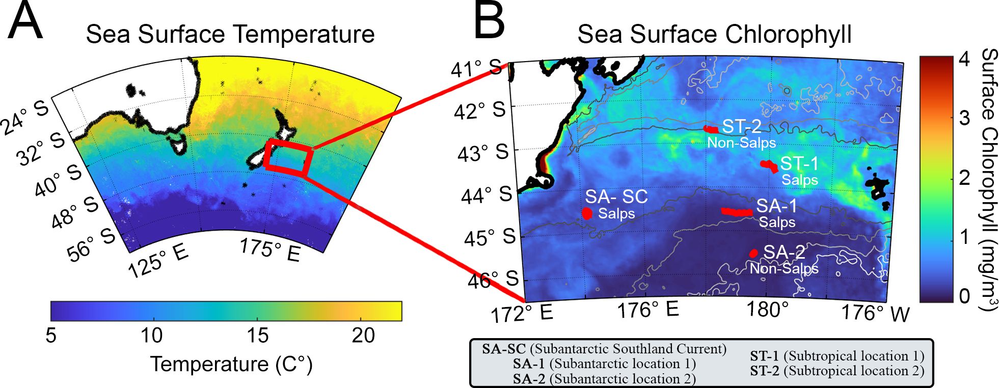
Figure 1. (A) General oceanographic region showing SST (sea surface temperature) at the time of sampling and (B) TAN1810 study region with October 2018 monthly averaged sea surface chlorophyll (NASA MODIS satellite data) and the five study locations, shown in red. Study sites are labeled as subtropical waters (ST) or subantarctic waters (SA). SA-SC = Subantarctic water with Southland Current influence. The presence or absence of salps in the study region is depicted in the figure as salps (present) or non-salps (absent).

The goals of this study were to, within the context of SA vs ST waters: 1) assess the depth-resolved variability of picoplankton (0.2 to 2 µm), nanoplankton (2 to 20 µm) and microplankton (>20 µm) abundance and C-based biomass in the euphotic zone, 2) evaluate the vertical, size-specific variability of carbon to chlorophyll a ratio (C:Chla), and 3) quantify the ratio of living to total particulate organic carbon (POC) during five Lagrangian-based experiments in different water parcels during austral spring in the SA (three locations) and the ST (two locations).

2 Materials and methods

2.1 Field collection

Data was collected in the Chatham Rise section of the Southern Ocean, located east of Aotearoa New Zealand, as part of the SalpPOOP (‘Salp Particle expOrt and Ocean Production’) voyage during October to November 2018 (Figure 1). We conducted five Lagrangian experiments (hereafter referred to as “cycles”) that each lasted four to eight days (Décima et al., 2023). Our sampling locations were mainly within the STF, in regions that were predominantly influenced by either ST or SA water masses. Our most coastal cycle, termed SA-SC, was impacted by the Southland Current (SC), a diversion of the STF constituted mainly by SA water (Sutton, 2003). Three cycles were sampled in SA waters (SA-SC, SA-1 and SA-2) and two cycles in ST waters (ST-1 and ST-2) (Supplementary Table 1, including station locations and characteristics). Two cycles in SA water (SA-SC and SA-1) and one cycle in ST water (ST-2) occurred within blooms of the salp Salpa thompsoni. In each cycle, satellite-tagged marker buoys were used to track the sampled water mass by tethering subsurface drogues centered at 15-m depth to each buoy to follow the mixed layer (ML) in a Lagrangian frame of reference (Landry et al., 2009; Stukel et al., 2015). The mixed layer depth was identified using CTD downcast data and determined as the depth where the change in density (sigma-t) exceeded the 10 m depth density by 0.125 kg m^-3 (Levitus, 1982) and the deep chlorophyll maximum (DCM) depth, when present, was determined by the depth of subsurface peak in chlorophyll a (Chla) fluorescence. Using this Lagrangian approach allowed us to sample the same water mass over time, to give context to the variability observed in our measurements. We used a 24-place 12-L Niskin bottle rosette equipped with a Seabird (SBE 911plus) CTD and profiling Chla fluorometer to obtain sample water at each station and chose six depths spanning the euphotic zone (surface to the 1% incident light level) based on Chla fluorescence measured during the downcast. The rosetteʻs sensors included SBE 3plus, SBE 4, and SBE 43 dual sensors for temperature, salinity, and dissolved oxygen, a Seapoint fluorescence sensor, and a photosynthetically active radiation (PAR) sensor (Biospherical Instruments QCP‐2300L‐HP). At each location, we conducted a single (~0:200), daily depth-resolved profile from the rosette, sampling for each parameter - epifluorescence microscopy (epi), flow cytometry (FCM), FlowCam, size-fractionated Chla and POC samples to quantify microplankton, nanoplankton and picoplankton biomass and abundance throughout the euphotic zone.

2.2 Sampling procedure

2.2.1 Epifluorescence microscopy sampling

From each depth, samples were obtained for epi: 50 mL for nanoplankton (filtered through a 0.8-µm pore-size black PCTE filter) and 400 mL for microplankton (filtered through an 8-µm pore-size black PCTE filter). The 8-µm pore size was chosen (rather than 20-µm pore size) to ensure that no microplankton passed through the filter either because of long, narrow shapes or as a result of compression of non-test bearing cells. 20 µm backing filters were utilized to support the membrane filters and ensure even dispersal of sample on the filter (Sherr et al., 1993; Taylor et al., 2015). The samples were preserved using sequential additions of borate-buffered formalin, alkaline Lugol’s solution, and sodium thiosulfate, then stained using proflavine and 4’, 6-diamidino-2 phenylindole (DAPI) (Sherr and Sherr, 1993). During and immediately after filtration, filters were covered with aluminum foil to prevent photochemical quenching. Filters were then mounted between immersion oil and a coverslip onto a glass slide and frozen (-80°C) for shore-based microscopy imaging analysis.

2.2.2 Flow cytometry sampling

Samples were collected for Synechococcus (Syn), Prochlorococcus (Pro), picophytoeukaryotes (peuk) and heterotrophic bacteria (hbact) using FCM since we are not able to confidently enumerate < 2-µm picoplankton using epi. Eukaryotic phytoplankton cells were analyzed alive with a shipboard FCM because preservation and freezing results in destruction of some cells and also modifies cell volumes (Vaulot et al., 1989). Prokaryotic cells show less preservation-related artifacts and enumeration of Pro required the use of a more sensitive, land-based flow cytometer. Thus, two types of samples were processed using FCM: live samples (2 mL) processed shipboard within 3 hours of collection to count eukaryotic phytoplankton and preserved (0.5% paraformaldehyde), flash-frozen (liquid nitrogen) samples (2 mL) that were analyzed for heterotrophic and photosynthetic prokaryotes on land. Live samples were processed using a Becton Dickinson Accuri C6 Plus flow cytometer, exciting at 488 nm and detecting Chla fluorescence (FL3, >670 nm LP) as the discrimination parameter, at a sample flow rate of 66 µL min^-1 for 10 min. Preserved samples were thawed in batches on shore, then stained with the DNA stain Hoechst 34580 for analyses on a Beckman Coulter CytoFlex S flow cytometer (Selph, 2021).

2.2.3 FlowCam sampling

A model V-4 FlowCam (Yokogawa Fluid Imaging Technologies) was utilized to count and image live plankton >4 µm in diameter. 2-3 replicate samples were collected (250 mL samples concentrated down to 10 mL using gravity filtration over a 2-µm pore size 47-mm filter, of which 2 mL were imaged) at two depths from each cast, which were typically within the ML and at the DCM. The samples were imaged at sea using the FlowCam’s 10x objective lens and processed on shore.

2.3 Analysis procedure

2.3.1 Epifluorescence microscopy imaging and analyses

Phytoplankton images from microscope slides were captured with an Olympus Microscope DP72 Camera mounted on an Olympus BX51 fluorescence microscope. 20 images were taken with filter sets appropriate for proflavine (482 nm excitation, 536 nm emission filters) in order to capture the fluorescence of cell proteins. Proflavine overstained the cells, obscuring Chla fluorescence, so it was not possible to differentiate heterotrophs from autotrophs, therefore only biomass and abundance values were obtained. A 60x objective lens was used to image slides from 0.8 µm filters for 2-12 µm cells, while a 20x objective lens was used to image slides from 8 µm filters for >12 µm cells.

Images were then processed using the ImageJ image analysis software (v 1.52a or 1.53c). Cells were manually outlined using the freehand tool and the approximate feret cell length and cell area were calculated in pixels and then converted to microns using a calibration scale. To avoid biasing the examined cell size, cells that were roughly >50% out of frame and cells that were broken or fragmented were not included in analysis. Conversion factors were applied to account for volume filtered and percentage of the filter area analyzed. To estimate the filtration area, a light microscope was used to examine a 25 mm glass fiber filter (GF/F) filter that had a small amount of dyed water filtered through, which revealed that the filtered region was circular with a diameter of 22 mm. Equations 1–5 were used to calculate cell width (W, Equation 1), biovolume (Equation 2), ESD (equivalent spherical diameter, Equation 3) and C biomass of diatoms (Equation 4) and all other cells (non-diatoms, Equation 5) using equations from Menden-Deuer and Lessard (2000). ESD was used as a consistent measure of mean cell size since many plankton have an irregular shape. For non-diatoms, the height of a cell was assumed to be roughly equivalent to half of the cell width since cells are often flattened during filtration (Taylor et al., 2011). For diatoms, we assumed that height equaled width.

$\begin{array}{ll}CellWidth=\frac{4}{\pi }\times \frac{Areaofthecell}{FeretLenghtofthecell}& (1)\end{array}$

$\begin{array}{ll}Biovlum{e}^{*}=\frac{4}{3}\pi \times (\frac{FeretLenght}{2})\times (\frac{CellWidth}{2})\times (\frac{CellHeigh{t}^{*}}{2})& (2)\end{array}$

$\begin{array}{ll}ESD=2\times {(\frac{3\ast Biovolume}{4\pi })}^{\frac{1}{2}}& (3)\end{array}$

$\begin{array}{ll}Biomass(diatoms)=0.288\times Biovolum{e}^{0.811}& (4)\end{array}$

$\begin{array}{ll}Biomass(non-diatoms)=0.216\times Biovolum{e}^{0.939}& (5)\end{array}$

2.3.2 Flow cytometry analyses

Populations of Syn, Pro, peuk and hbact were distinguished by their different auto- (Chla, phycoerythrin) and stain-fluorescence (DNA) and light-scattering (forward and side scatter) signatures using FlowJo software. These abundance values were then converted to biomass estimates using C conversion values of 36 and 11 fg C cell^-1 for Pro, and hbact, respectively (Garrison et al., 2000; Buitenhuis et al., 2012). For Syn and peuk cells, the biomass was estimated allometrically from cell diameter (as estimated from bead-calibrated forward light scatter signals) using equations (Equation 5) in Menden-Deuer and Lessard (2000) and Bertilsson et al. (2003).

2.3.3 Normalized biomass and abundance size spectra (NBSS and NASS)

For every cycle and depth, Normalized Biomass Size Spectra (NBSS) were calculated for nanoplankton and microplankton biomass. Biomass was binned by ESD into different size bins, (e.g., 2 to 4 µm, 4 to 8 µm, 8 to 16 µm, etc.), summed for each size bin and then divided by the width of the given size bin (e.g., 2 µm, 4 µm and 8 µm, respectively, for the previous example). Normalized Abundance Size Spectra (NASS) were similarly calculated albeit using counts of cells rather than their biomass. Thus, each point in the figures for NBSS and NASS represents the average of the summed biomasses for the corresponding size range, divided by the bin width.

We quantified uncertainty by calculating 95% confidence intervals in NASS and NBSS using Markov Chain Monte Carlo random resampling. Briefly, a new simulated dataset of cells of the same number of data points (i.e., cells per image, images per slide, and casts per cycle) to the actual dataset was derived by randomly sampling with replacement the indexes according to the following order: 1) a CTD cast in each cycle, 2) 1 of the 20 images taken, and 3) a particular cell. The simulated dataset was then sorted into appropriate ESD size bins, NASS and NBSS were calculated, and the procedure was repeated 10,000 times. This process generates 10,000 new datasets that are similar to the original dataset in range and size. The lower confidence interval, 2.5^th percentile, and the higher confidence interval, 97.5^th percentile, of the 10,000 values of NASS or NBSS represents the bounds for lower and upper confidence intervals creating our 95% confidence interval ranges.

2.3.4 FlowCam analyses

FlowCam images were processed in VisualSpreadsheet (v. 4.18.5) where images were individually examined, duplicate cells were deleted, and taxonomic classification determined (Fender et al., 2023). The length and width measurements were calculated using the formula for a prolate spheroid (Equations 2, 3) with the exception that for width we used the minimum feret length of the particle with no correction for flattening. Any identifiable tintinnid ciliates, rhizarians and obligate heterotrophic dinoflagellate taxa were removed to provide a more accurate estimate of autotrophic C biomass. The C biomass of the remaining particles was estimated using the same allometric conversions for diatoms and non-diatoms as in epi analysis.

2.3.5 Biomass and C:Chla analysis

For the estimation of picoplankton biomass, we utilized FCM data for hbact, Syn, Pro and peuks. However, when determining picophytoplankton C:Chla, hbact were excluded. To determine diatom, nanoplankton and microplankton biomass and abundance, we relied on epi data, assuming that most FCM data for peuks represented cells ≤2 µm in diameter. In addition, we implement independent FlowCam C estimates (cells ≥4 µm) focusing specifically on nanoplankton and microplankton sized cells and compare to epi C:Chla. The statistics of the ratios are derived from the ratio of mean carbon divided by mean Chla for each depth and cycle. A summary of the methods used in this study to determine plankton carbon estimates can be found in Supplementary Table 2.

2.4 POC measurements

POC was estimated by filtering a seawater sample (2.2 L) onto a pre-combusted 25-mm GF/F filter under low vacuum pressure (5 to 7” Hg), using similar depths as CTD casts for FCM, FlowCam and epi. These filters were deep frozen (-80°C) for later analysis. On shore, samples were thawed, acidified with fuming HCl in a desiccator, excess acid removed under vacuum pressure and finally the samples were placed in a drying oven for 24 h at 40°C. The samples were then packaged into a tin capsule and analyzed at the University of California Davis Stable Isotope Facility for C content measured with an elemental analyzer coupled to an isotope ratio mass spectrometer.

2.5 Size fractionated chlorophyll a measurements

Samples for size fractionated Chla were analyzed by first gravity filtering a sample (250 mL) through a 20 µm 47-mm polycarbonate filter, then with low vacuum pressure, filtering sequentially through a 2 µm and a 0.2 µm polycarbonate filter. Filters were then folded, placed in 1.5 mL cryovials and frozen (-80°C) until analysis (Gutiérrez-Rodríguez et al., 2020). Chla and acidified phaeopigment-a concentrations were measured (within 3 months) using ice-cold 90% acetone extraction by spectrofluorometric methods (APHA 10200 H) on a Varian Cary Eclipse fluorescence spectrophotometer (Rice et al., 2012).

2.6 Nutrient measurements

Nutrient samples were gravity filtered using a 0.2 µm Acrocap in-line capsule (Pall-Gelman) connected to a Niskin bottle by an acid-rinsed silicon tube into a 50-mL falcon tube that was first triple-rinsed with filtered seawater, filled halfway, capped and sealed with parafilm and stored at -80°C until analysis. Nutrient samples were analyzed for nitrate (NO₃⁻), ammonium (NH₄⁺), dissolved reactive phosphorus (DRP) and silicic acid (DRSi) concentrations using an Astoria Pacific API300 micro segmented flow analyzer (Astoria‐Pacific, Clackamas, OR, USA). Analyses were completed by the National Institute of Water and Atmospheric Research (NIWA) in Hamilton (New Zealand) following standard procedures (Law et al., 2011).

3 Results

3.1 In situ conditions

High oxygen saturation % in the upper euphotic zone during the SA-SC cycle relative to other cycles, along with higher fluorescence seen in Chla relative to other SA cycles, suggest that this cycle had higher autotroph biomass typical of coastal upwelling and/or mixing associated with the SC (Table 1; Figure 2). SA-SC, SA-1 and SA-2 displayed traits characteristic of colder, Southern Ocean water masses with lower average temperature as a function of depth, higher oxygen saturation % and lower salinity concentrations relative to the ST cycles (Figure 2). The water parcel in SA-SC traveled up the eastern coast of Southern New Zealand and diverged when meeting the STF. While both of our SA cycles were located further offshore than our SA-SC cycle, SA-2 is a better representation of typical SA waters while SA-1 is likely influenced by mixing with the STF as indicated by high fluorescence and oxygen saturation % (Figure 2; Table 1). ST-1 and ST-2 cycles displayed overall lower oxygen saturation %, higher temperatures, and higher salinity throughout the water column (Figure 2). SA cycles generally had higher surface concentrations of DRP, NO₃^- and NH₄⁺ and DRSi compared to ST cycles while surface Chla measurements were higher in ST cycles compared to SA cycles (Table 1).

Table 1

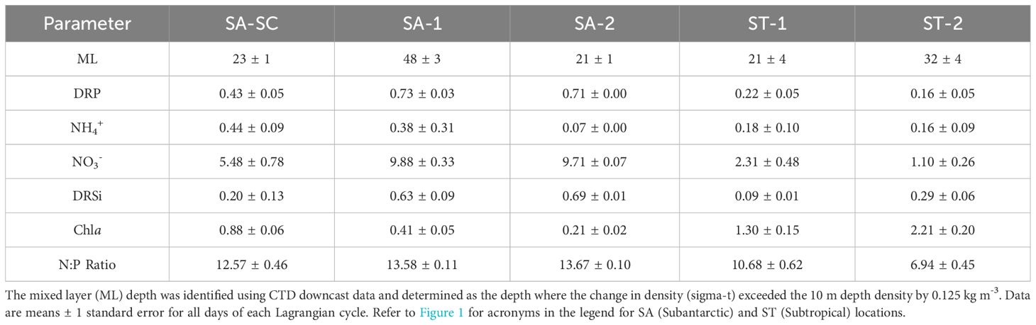
Table 1. Average surface (5 m) euphotic nutrient concentrations for dissolved reactive phosphorus (DRP, µM), nitrogen (NO₃^- and NH₄⁺, µM) and dissolved reactive silicate (DRSi, µM), average summed size-fractionated surface (5 m) Chla (µg C L^-1) and the average N:P ratio.

Figure 2

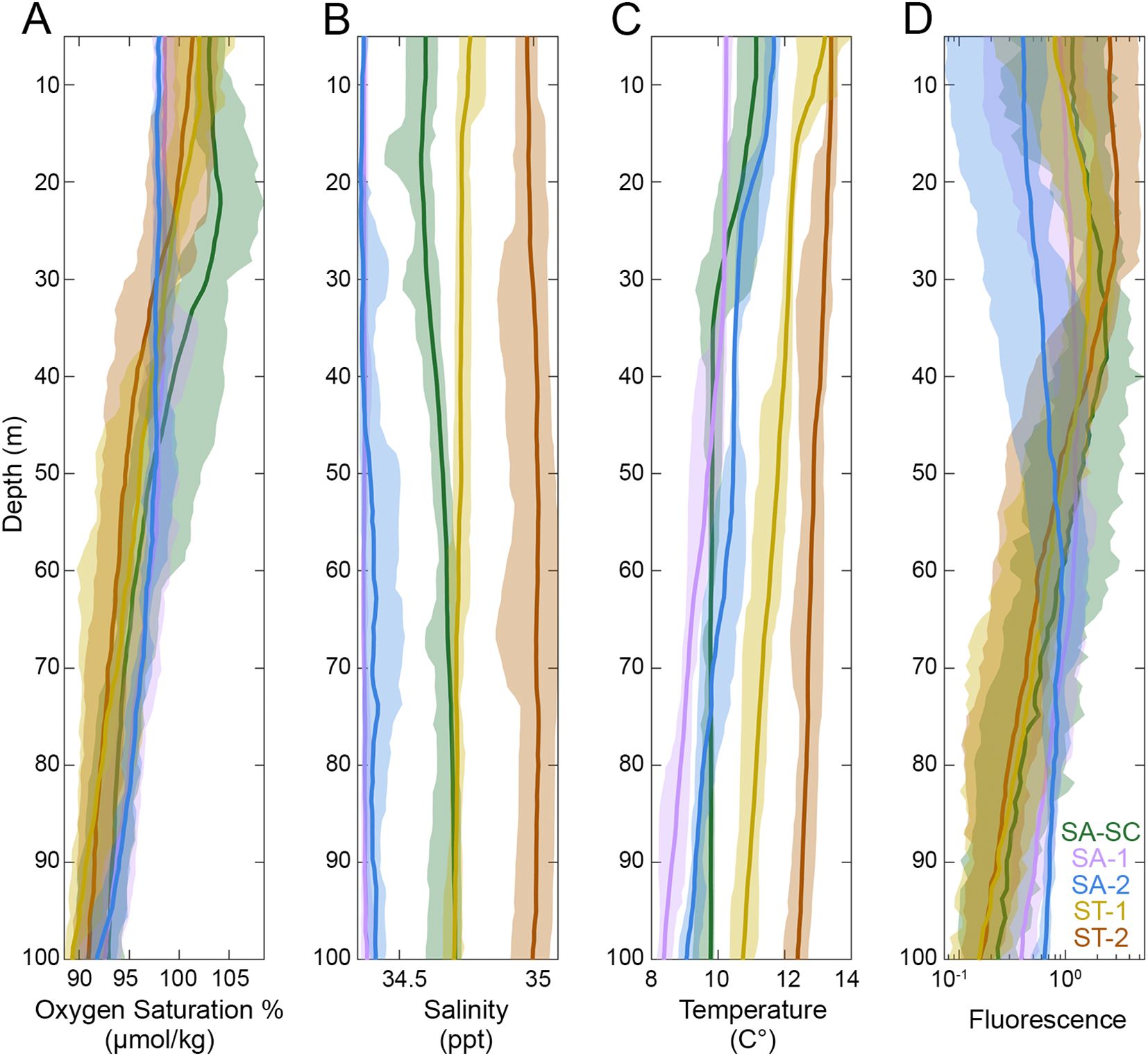
Figure 2. (A) Oxygen, (B) salinity, (C) temperature, and (D) fluorescence profiles for each cycle. Lines represent the mean data while the shaded region represents 95% confidence intervals. Colors denote the different regions sampled for SA (Subantarctic) or ST (Subtropical). Refer to Figure 1 for acronyms in the legend. The x-axis in the fluorescence panel is in logarithmic scale.

3.2 Vertical distribution of abundance and biomass of the plankton community

Phytoplankton biomass and abundance data provided additional evidence of the distinct separation of SA and ST water masses. Abundance data suggests that nanoplankton had higher counts in ST (mean ± 1 standard error; 973.69 ± 112.27 cells mL^-1) compared to SA (604.43 ± 46.91 cells mL^-1) (Figure 3). Diatoms showed the opposite pattern with higher abundances in SA (12.7 ± 2.54 cells mL^-1) compared to ST (0.17 ± 0.06 cells mL^-1), although diatoms were also rare in SA-2. Microplankton showed no significant difference in abundance between SA (8.43 ± 0.61 cells mL^-1) and ST (8.88 ± 1.05 cells mL^-1). Overall, when analyzing the vertically averaged biomass, which is calculated by taking the average biomass across all euphotic depths, picoplankton (as a summed group) exhibited the highest biomass in the two offshore SA cycles averaged together (18.5 ± 0.9 µg C L^-1) compared to nanoplankton (16.6 ± 1.3 µg C L^-1) and microplankton (13.0 ± 1.1 µg C L^-1) (Figure 4). However, nanoplankton biomass (35.2 ± 4.6 µg C L^-1) was highest in ST cycles compared to picoplankton (28.9 ± 1.1 µg C L^-1) and microplankton (14.4 ± 1.6 µg C L^-1). Diatoms had higher vertically averaged biomass in all SA cycles (0.8 ± 0.1 µg C L^-1) compared to ST cycles (0.1 ± 0.04 µg C L^-1) (Figure 4) and higher abundance in SA (12.7 ± 2.5 cells mL^-1) compared to ST (0.9 ± 0.51 cells mL^-1) (Figure 3). Although diatoms had similar abundances in the upper water column for SA-SC and SA-1 (Figure 3), vertical biomass distributions suggested that diatoms had higher biomass in SA-SC compared to SA-1 (Figure 4). Generally, microplankton biomass did not differ between SA and ST regions (16.2 and 14.4 µg C L^-1, respectively) and had the highest vertically averaged biomass at the SA-SC water parcel (21.7 ± 2.2 µg C L^-1) (Figure 4). The abundance of microplankton was also comparable between the SA and ST cycles (8.43-8.88 cells mL^-1) (Figure 3). In SA cycles, nanoplankton vertically averaged biomass (15.6 ± 0.9 µg C L^-1) was comparable to microplankton biomass (16.2 ± 1.2 µg C L^-1) but was nearly two-fold higher in ST cycles (35.2 ± 4.6 µg C L^-1 and 14.4 ± 1.6 µg C L^-1, respectively) (Figure 4).

Figure 3

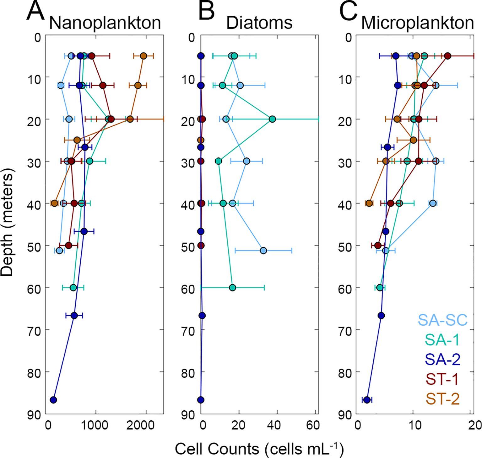
Figure 3. Average abundance of (A) nanoplankton, (B) diatoms and (C) microplankton groups as a function of depth estimated from epifluorescence microscopy. Refer to Figure 1 for acronyms in the legend. Cool colors (shades of blue) represent SA (Subantarctic) cycles and warm colors (shades of red) represent ST (Subtropical) cycles. Error bars represent one standard error of the mean. Note the differences in x-axis scales.

Figure 4

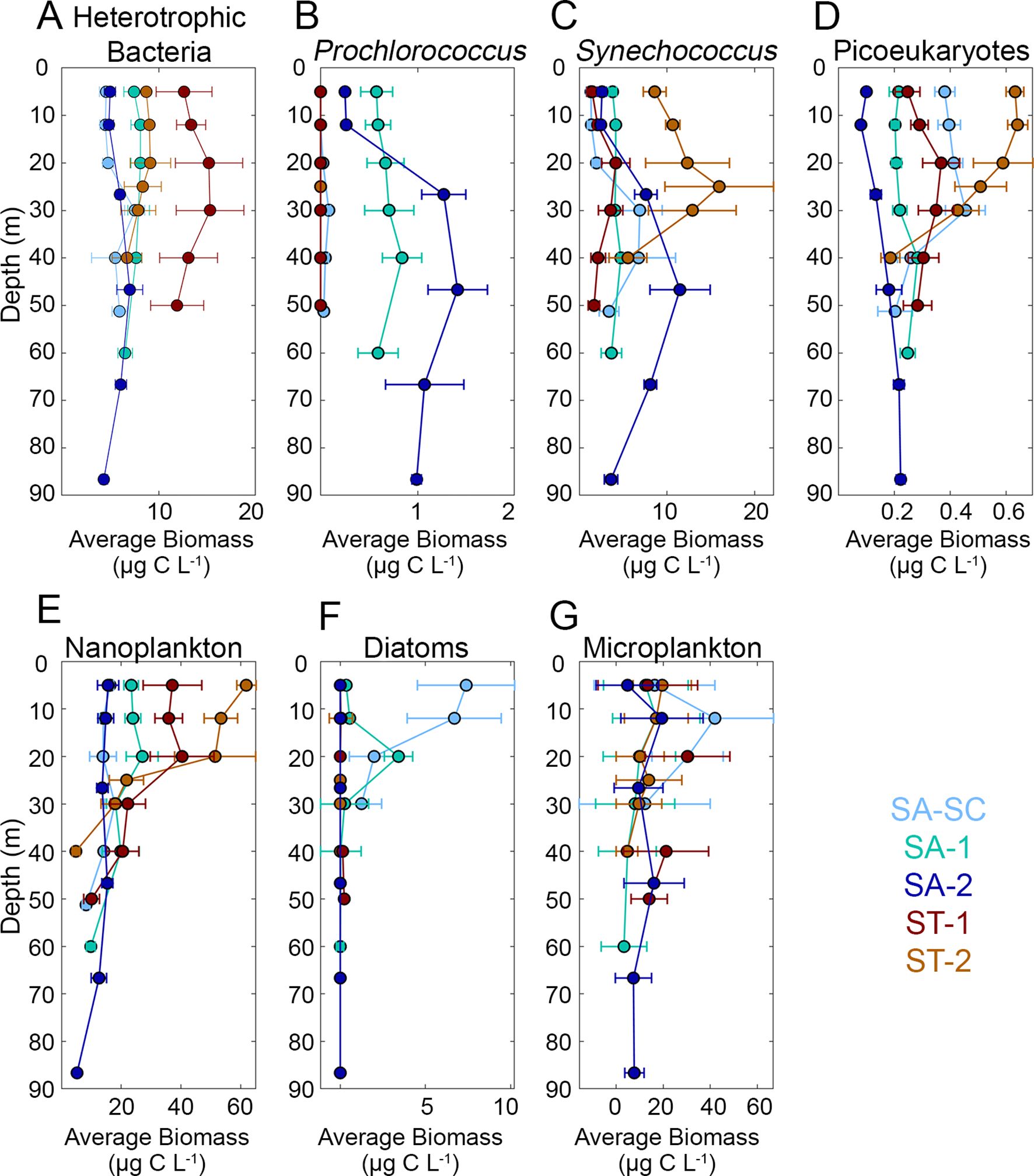
Figure 4. Average microbial biomass results from flow cytometry data ((A) heterotrophic bacteria, (B) Prochlorococcus, (C) Synechococcus and (D) picoeukaryotes) and epifluorescence microscopy ((E) nanoplankton, (F) diatoms and (G) microplankton) for each study region. Refer to Figure 1 for acronyms in the legend. Cool colors (shades of blue) represent SA (Subantarctic) cycles and warm colors (shades of red) represent ST (Subtropical) cycles. Error bars represent one standard error of the mean. Note the differences in x-axis scales.

Picoplankton groups suggested that hbact water column biomass was 2-fold higher in ST (22.0 ± 1.5 µg C L^-1) relative to SA cycles (12.4 ± 0.5 µg C L^-1). Pro was found in SA cycles (0.6 ± 0.1 µg C L^-1), particularly in the cycles conducted further offshore and away from the STF, but it was not present in ST cycles (Figure 4). Syn had slightly higher overall vertically averaged biomass in ST cycles (6.5 ± 1.2 µg C L^-1) compared to SA cycles (4.5 ± 0.5 µg C L^-1) (Figure 4). Peuk were present at very low concentrations in all regions with slightly higher vertically averaged biomass in the ST (0.4 ± 0.04 µg C L^-1) compared to the SA (0.2 ± 0.002 µg C L^-1). Average C biomass and abundance for each group and water parcel can be found in Supplementary Table 3.

Normalized size spectra allow us to visualize the abundance and total biomass of cells in a specific size range. The biomass size spectrum reflects the energy flow within the system, with the slope providing information on growth and mortality dynamics and trophic efficiency within the community. This can also signify trophic recycling processes within the system (Zhou, 2006). The relative shape of the curve describes the degree to which community composition is dominated by small or large phytoplankton, with a less negative slope indicating a relatively greater importance of large cells (microplankton dominance) and vice versa (note that the smallest size class in both NBSS (Figure 5) and NASS (Figure 6) represent flow cytometric picoplankton in the size range of 0.5 to 2 µm that contains the averaged sum of hbact, Syn, Pro and peuk). The overall average slope of NBSS of all ST cycles was -0.78, which is less negative than the overall average slope of SA cycles (-1.00) and suggests a greater relative proportion of larger cells in ST relative to SA cycles (Supplementary Table 4). Similarly, the average slope of NASS of all SA cycles was -3.26 and slightly more negative compared to ST cycles (-3.04). A table that contains all slope values can be found in the Supplementary Material (Supplementary Table 4). While NBSS did not show monotonic changes with depth, the NBSS was typically more negative at the DCM than in the mixed layer suggesting that small cells contributed proportionally more to biomass in the deep euphotic zone than the shallow euphotic zone. The NBSS plots also show consistently low biomass of small nano cells (2 – 4 µm cells) across all cycles and depths.

Figure 5

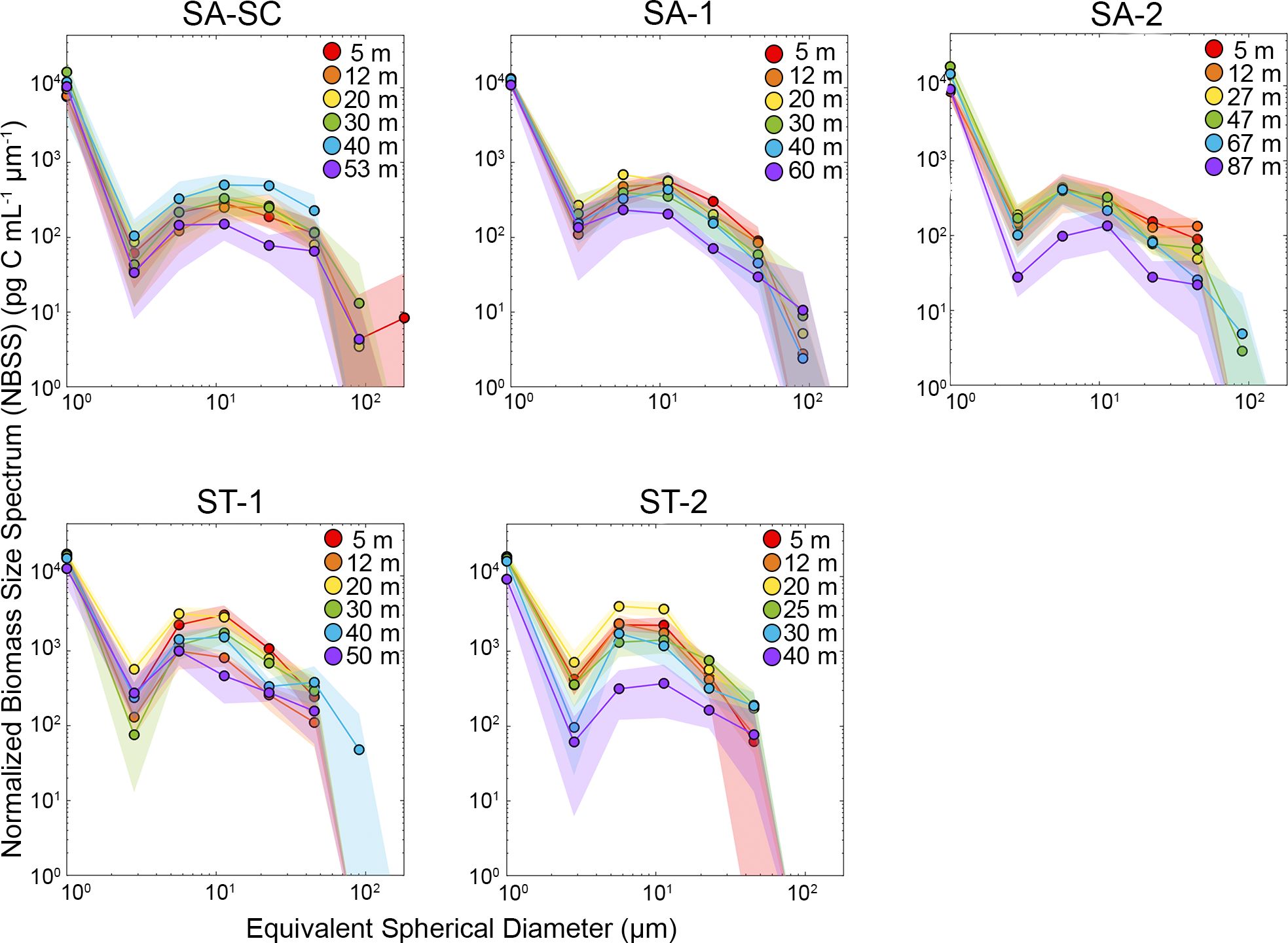
Figure 5. Cycle-average NBSS (Normalized biomass size spectra) for the entire microbial community as a function of depth. Shaded regions represent 95% confidence intervals. Both scales are in logarithmic units. C data is from epifluorescence microscopy and flow cytometry for the smallest size class. Refer to Figure 1 for acronyms in the legend for SA (Subantarctic) and ST (Subtropical) locations.

Figure 6

Figure 6. Normalized Abundance Size Spectra (NASS) for the entire microbial community as a function of depth. Shaded regions represent 95% confidence intervals. Both scales are in logarithmic units. Data is from epifluorescence microscopy and flow cytometry for the smallest size class. Refer to Figure 1 for acronyms in the legend for SA (Subantarctic) and ST (Subtropical) locations.

3.3 Vertically averaged biomass of picoplankton, nanoplankton and microplankton

Vertically averaged summed biomass, calculated by taking the vertical integrations of biomass above the ML and below the ML and then diving by the two depths, showed differences between picoplankton, nanoplankton and microplankton within the ML compared to below the ML (Figure 7). ML depths can be found in Table 1. Picoplankton had slightly lower vertically averaged biomass within the ML (Hbact 16.5 ± 3.2 mg C m^-3, Syn 4.5 ± 1.9 mg C m^-3, Pro 0.2 ± 0.1 mg C m^-3, peuk 0.2 ± 0.1 mg C m^-3) compared to below the ML (Hbact 17.6 ± 3.3 mg C m^-3, Syn 7.2 ± 1.7 mg C m^-3, Pro 0.4 ± 0.3 mg C m^-3, peuk 0.3 ± 0.04 mg C m^-3) (Figure 7A), which is more clearly seen in relative proportion with picoplankton contributing to more vertically averaged biomass below the ML (42% on average) compared to the ML (30% on average) (Figure 7B). Conversely, nanoplankton and microplankton had higher biomass in the ML (nanoplankton 29.1 ± 7.0 mg C m^-3, microplankton 18.4 ± 2.1 mg C m^-3) compared to below the ML (nanoplankton 19.3 mg C m^-3 ± 2.4, microplankton 15.3 ± 2.6 mg C m^-3). Diatoms had similar vertically averaged biomass in the ML (0.9 ± 0.6) and below (1.1 ± 0.6). Picoplankton as a group contributed to more vertically averaged biomass below the ML while the larger plankton groups (nanoplankton, diatoms and microplankton) contributed to more biomass in the ML (Figure 7B). ST water samples had higher vertically average summed biomass in the ML compared to SA water samples (92.7 ± 3.2 mg C m^-3 and 54.7 ± 5.4 mg C m^-3, respectively) and below the ML (ST: 69.6 ± 11.5 mg C m^-3, SA: 55.3 ± 3.9 mg C m^-3).

Figure 7

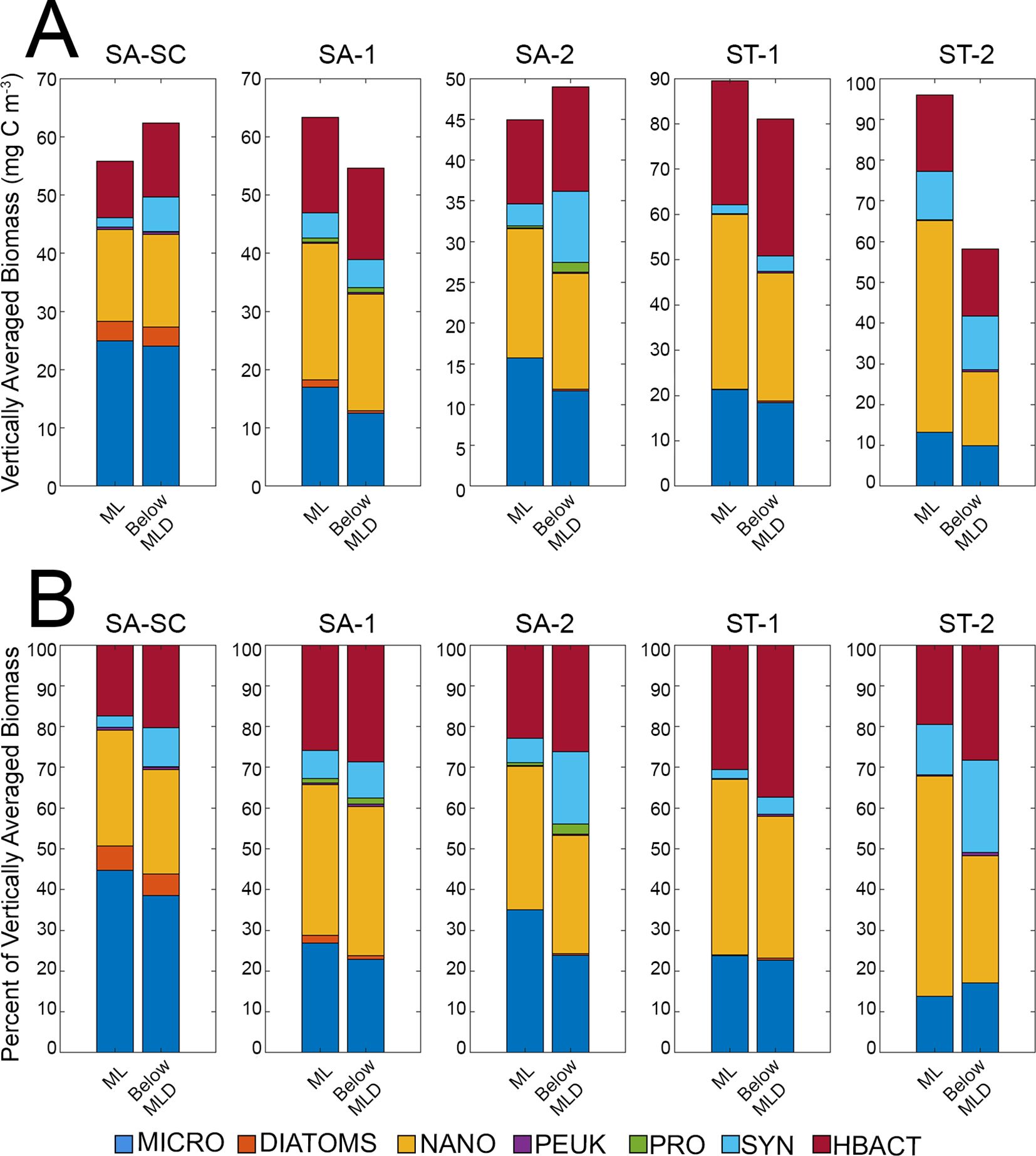
Figure 7. (A) Vertically averaged biomass (mg C m^-3) of each measured group (heterotrophic bacteria, Prochloroccus, Synechococcus, picoeukaryotes, nanoplankton, diatoms and microplankton) was determined by vertically integrated through the mixed layer (ML) and below the mixed layer depth (Below MLD). The calculated result was then divided by the respective depth of the ML and below MLD. (B) Contribution of each group measured to the total vertically integrated biomass presented in the MLD and below the MLD. MLD are 23, 48, 21, 21 and 32 m for SA-SC, SA-1, SA-2, ST-1 and ST-2, respectively. Refer to Figure 1 for acronyms in the legend for SA (Subantarctic) and ST (Subtropical) locations.

3.4 Carbon to chlorophyll a ratios

While our epi measurements enabled high vertical resolution of C:Chla variability, they should be treated as upper bounds for the actual C:Chla ratios of nanoplankton and microplankton because they include heterotrophic protists (i.e., due to overstaining with proflavine, we were unable to use Chl autofluorescence to discriminate phototrophs from obligate heterotrophs). Our C:Chla values are calculated by taking the ratio of mean carbon divided by mean Chla for each depth and cycle. Picoplankton consistently exhibited lower average C:Chla ratios in the ML compared to the nanoplankton and microplankton in both the ST and SA regions (Figure 8A). Microplankton generally had higher C:Chla ratios compared to nanoplankton, although this relationship varied depending on location and depth, which is likely due to size fractionated Chla differences (Figure 8A). Picoplankton had the highest C:Chla signal at 30 m (SA: 48.9 ± 12.1; ST: 19.1 ± 7.4), nanoplankton at 20 m (SA: 354.3 ± 67.2; ST: 168.6 ± 89.9) and microplankton at 12 m (SA: 1044.6 ± 474.1; ST: 501.2 ± 241.7) (Figure 8A). In general, SA cycles had higher overall average C:Chla for all groups (e.g., at 12 m: picoplankton 18.4 ± 4.8, nanoplankton 319.6 ± 49.0, microplankton 1044.6 ± 474.1) compared to ST regions (12 m: picoplankton 12.1 ± 3.7, nanoplankton 156.4 ± 26.0, microplankton 501.2 ± 241.7) (Figure 8A).

Figure 8

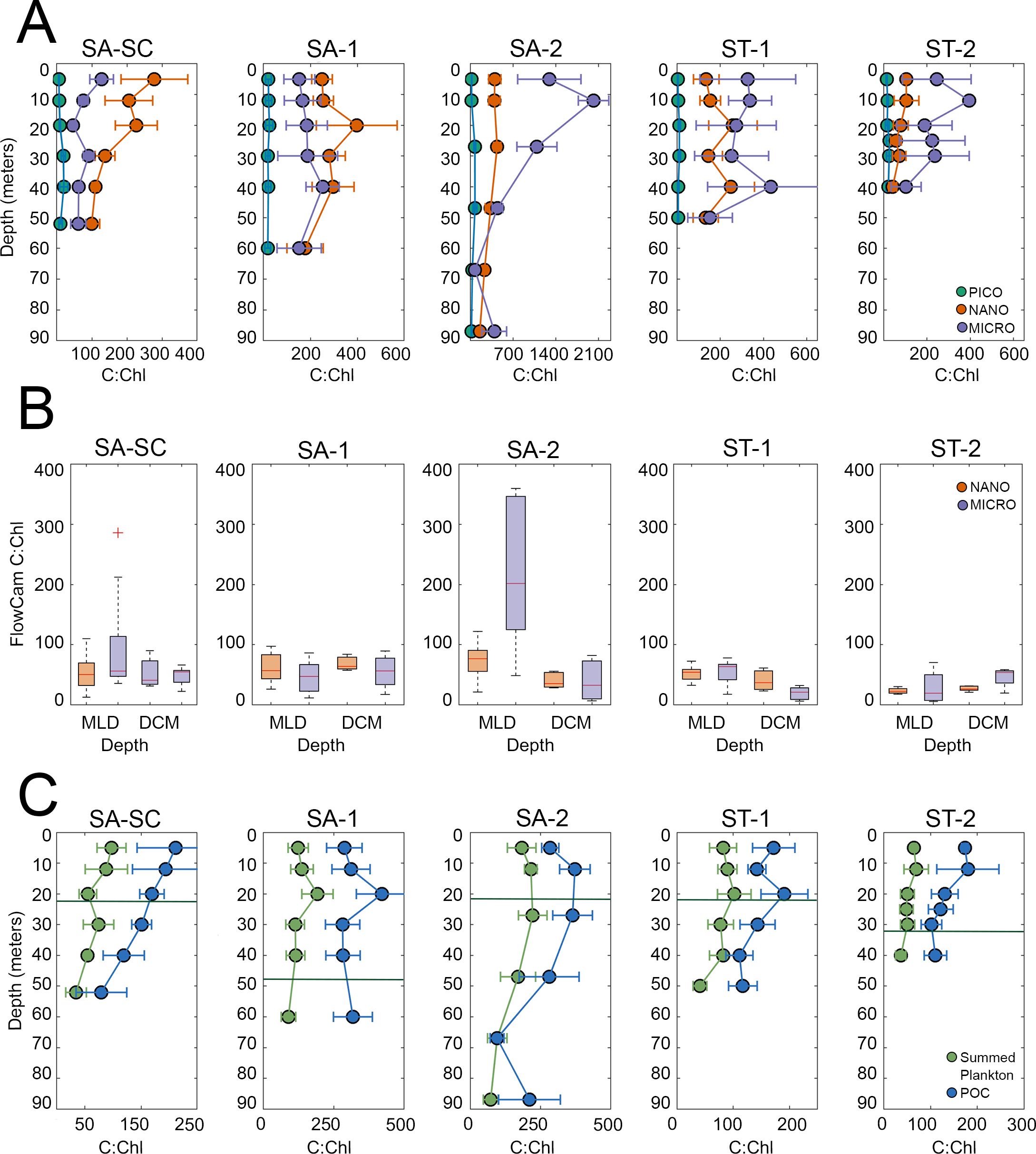
Figure 8. Cycle-averaged C:Chla profiles obtained using C estimates from (A) epifluorescence microscopy and flow cytometry biomass data for size fractionated chlorophyll for picoplankton (pico, 0.2-2.0 µm), nanoplankton (nano, 2-20 µm) and microplankton chlorophyll (micro, >20 µm) (B) FlowCam C biomass for nanoplankton and microplankton and (C) summed plankton C from epifluorescence microscopy and flow cytometry (green) and POC (blue) with summed size fractionated chlorophyll. Solid dark green line represents the mixed layer depth, exact depths can be found in Table 1. Error bars represent the uncertainty propagated from standard error. Note the differences in x-axis scales. Refer to Figure 1 for acronyms in the legend for SA (Subantarctic) and ST (Subtropical) locations.

We employed FlowCam samples to calculate C:Chla ratios as an alternative method of estimating C biomass, which mitigates biases associated with including heterotrophs compared to the epi data (Figure 8B). However, FlowCam data was limited to 2 depths (ML and DCM) and does not include ≤4 µm cells. FlowCam data revealed higher C:Chla ratios in SA compared to ST waters for both nanoplankton and microplankton and at both depths. Nanoplankton C:Chla was highest in the ML for SA-2 (73.5 ± 11.1) and lowest in the DCM of ST-2 cycle (23.1 ± 2.7) (Figure 8B). Microplankton C:Chla was highest in the ML of SA-2 (219.2 ± 43.9, Figure 8B); a peak in C:Chla ratio that is also seen in epi-based C:Chla estimated for microplankton (1044.6 ± 474.1, Figure 8A), and was lowest in the DCM of ST-1 (19.2 ± 3.6). In the ML of the SA region, the C:Chla ratio for microplankton was approximately twice as high as that for nanoplankton (120.3 ± 21.6 and 61.7 ± 5.8, respectively) although nanoplankton and microplankton C:Chla were similar in the ST regions (microplankton, 46.2 ± 7.5 and nanoplankton, 42.3 ± 5.1).

To allow comparison to other studies that lack size-resolved C:Chla ratios, we also present phytoplankton C:Chla ratios as the sum of epi (microplankton, nanoplankton and diatoms) and FCM (Syn, Pro and peuk) biomasses divided by total Chla (Figure 8C). We also compared C:Chla ratios determined from POC:total Chla to determine how well our estimations of phytoplankton C paired with overall POC to Chla depth profiles (Figure 8C). A point to consider when examining different methods used to calculate C:Chla is the use of different types of filters (e.g., polycarbonate vs. GF/F filters), which may influence the derived ratios due to variations in pore size and protein-binding activity, especially in samples with high dissolved organic matter (Chow et al., 2005). This variation in filter type is often unavoidable when sampling for POC, silicate, and other parameters, yet it may impact the results for bulk C:Chla values. Both summed phytoplankton and POC C:Chla had much higher average surface (~5 m) values in SA (144.0 ± 18.6 and 267.5 ± 20.8, respectively) compared to ST (70.9 ± 6.8 and 173.1 ± 4.1, respectively). Overall, POC C:Chla was higher than summed phytoplankton C:Chla, which is expected as POC includes hbact and detritus whereas summed phytoplankton contains only autotrophic C (and, in the case of our epi samples, also includes some heterotrophic protists). A detailed summary table of our various methods of estimating C:Chla can be found in Supplementary Table 5.

3.5 Living vs. total carbon

To quantify the proportion of the seston that is alive versus dead (i.e., detritus, including dead cells, fecal pellets, etc.), living biomass (microplankton, diatoms, nanoplankton, Pro, Syn, hbact and peuk) was summed and compared to bulk POC measurements. Across all locations and 6 depths, the median ratio of living:total C was 0.67 ± 0.03, which suggests that roughly 33% of the seston is detrital (Figure 9). We had initially hypothesized that salps might increase the ratio of living:dead organic C, because their high filtration rates and rapidly sinking fecal pellets could efficiently remove detritus from the euphotic zone. We used a Mann-Whitney U test to compare the differences in living and total C between water parcels with and without salps. The results indicated a possibly meaningful decrease in the proportion of living seston in the presence of salps, although the difference was not statistically significant at the 95% confidence level (p-value = 0.48). In contrast to differences between salp-influenced and non-salp water parcels, we found no meaningful difference in percent living seston between SA (0.70 ± 0.04) and ST samples (0.66 ± 0.05; p-value = 0.84).

Figure 9

Figure 9. The relationship between living POC and total POC (directly measured from GF/F filters). Summed plankton C estimates are from flow cytometry (heterotrophic bacteria, Prochlorococcus, Synechococcus and picoeukaryotes) and epifluorescence microscopy (nanoplankton, diatoms and microplankton). Blue markers represent locations with salps, red markers represent locations without salps, triangles represent SA (Subantarctic) water masses and circles represents ST (Subtropical) water masses, refer to Figure 1 for acronyms in the legend. The red line indicates the 1:1 ratio.

4 Discussion

4.1 Community composition

Our results suggest that ST cycles were dominated by nanoplankton, which is in agreement with previous research finding that nanoplankton comprised ~30% of total phytoplankton biomass in STF locations, compared to ~20% of total phytoplankton biomass in SA locations (Hall et al., 1999). Notably, our cycles sampled the STF zone, which is characterized by active mesoscale processes that mix ST and SA waters. Consequently, when appropriate, our samples are considered ST-influenced or SA-influenced within the STF when comparing our data to previous published research. Offshore SA cycles were dominated by picoplankton, while the SA-SC cycle, which was impacted by the Southland Current, was dominated by microplankton. High microplankton biomass in the SA-SC likely resulted from potential mixing of elevated nitrate and silicate SA waters with iron-enriched waters from the coastal domain and/or Southland Current, a subantarctic current that transports mainly SA (90%) but also ST (10%) waters (Sutton, 2003). In contrast, SA-1 and SA-2, which were located further offshore, were more oligotrophic than SA-SC and were dominated by picoplankton thriving in a high-nutrient, low-chlorophyll (HNLC) region, where iron is likely the limiting factor to phytoplankton growth (Boyd et al., 2010; Gutiérrez-Rodríguez et al., 2020). Although past research in this region of the SW Pacific suggests that microplankton biomass varies between oceanographic regions/water masses and can contribute ~5% of total cell C in STF regions and ~45% of total cell C in SA regions (Hall et al., 1999), during our study, microplankton did not vary greatly between regions (SA: 13.0 ± 1.1 µg C L^-1; ST: 14.4 ± 1.6 µg C L^-1) despite having the highest biomass in our SA-SC cycle (21.7 ± 2.2 µg C L^-1).

Our analysis of the NBSS and NASS spectra further elucidates the structure within these plankton communities by highlighting the distributions of biomass and abundance across different plankton size classes. For example, the lower NBSS slope observed in ST cycles (-0.78) compared to SA cycles (-1.00) suggests that there is a greater contribution of larger cells which potentially indicates higher trophic efficiency and a reduced loss of energy through trophic transfers in the ST cycles (Zhou, 2006). This aligns with our observations of increased nanoplankton dominance in ST cycles and picoplankton dominance in SA cycles, further supported by the more negative NASS slope in SA (-3.26) compared to ST (-3.04). The slope at the DCM can also provide insights into the vertical community structure. We observed that, apart from ST-2, the NBSS slopes tend to be more negative at the DCM which may suggest that there is a greater proportion of smaller cells at the DCM compared to the surface. This depth-related shift in size structure may suggest that smaller cells are better adapted to lower light levels found at the DCM, a pattern that we found in the vertical distribution of our picoplankton biomass as well. These insights from NBSS and NASS deepen our understanding of the community composition dynamics within each region and can illustrate how the size structure may influence carbon cycling and energy transfer across trophic levels.

Diatoms were present at low abundance in both regions with slightly higher biomass in SA cycles. Our results are in agreement with low values of diatoms reported in the SA region (Kopczynska et al., 2001; Peloquin et al., 2011; Cassar et al., 2015). In contrast, Chang and Gall (1998) found that vertically averaged diatom biomass was much higher in ST compared to SA (ST: 2804 μg C L^-1; SA: 13 μg C L^-1), unlike our study which found 10-fold lower average vertically averaged diatom biomass in ST compared to SA (ST: 0.1 ± 0.1 µg C L^-1; SA: 1.4 ± 0.6 µg C L^-1). Chang and Gall (1998) study occurred during a stronger spring bloom, with diatom biomass comprising 68% of total plankton biomass in the ST region, and their DRSi ambient concentration was 6-fold higher than in our study. The draw-down of DRSi and the relatively low abundance of diatoms during our study indicates a fading diatom bloom similar to that reported by Chang and Gall (1998) and Twining et al. (2014). The ST-1 average DRSi concentration of 0.09 ± 0.01 µM is below what is considered DRSi limiting (i.e., <0.2 µM), which is rare to find anywhere in the ocean (Nelson and Dortch, 1996). Despite the high concentration of Chla in ST-2 (2.21 ± 0.20 µg C L^-1, Table 1), diatoms were not abundant unlike previous reports (e.g. Chang and Gall, 1998; Twining et al., 2014) and instead the community was dominated by small flagellates and dinoflagellates. This highlights temporal variability in spring bloom dynamics and plankton community composition, particularly the diatom contribution, in this dynamic region (Chiswell et al., 2019; Gutiérrez-Rodríguez et al., 2022).

Pro was present in SA cycles but absent in all ST cycles (Figure 3). This finding is unexpected because Pro is typically observed in warmer, oligotrophic regions, although it has been found to occur in colder waters, down to ~10°C (Doolittle et al., 2008). More often though, Pro is found in warmer ST waters in the Tasman Front, suggesting that its abundance in SA waters may be constrained by temperature (Dubreuil et al., 2003; Yang et al., 2010; Ellwood et al., 2013). In SA cycles, Pro typically had higher biomass deeper in the water column compared to the surface, e.g., for SA-2, average Pro biomass was ~5.6-fold lower at 5 m compared to 46 m (0.3 ± 0.02 and 1.4 ± 0.3 µg C L^-1, respectively).

Macronutrient limitation may explain the lower microplankton biomass seen in ST cycles, particularly nitrogen as indicated by the NO₃^-:PO₄⁺ ratios in Table 1 which are well below the Redfield ratio and suggest nitrogen limitation may be occurring in this region. In contract, SA cycles are likely limited by trace metals, such as iron, which is characteristic of SA water masses (Banse, 1996; Sedwick et al., 2000; Nodder et al., 2007; Ellwood et al., 2013) and is likely responsible for the reduced biomass of microplankton seen in the offshore SA cycles. Additionally, potential silica limitation in both ST and SA waters, as seen in low silica concentrations (Table 1), could impact diatom productively offshore. It was only in the SA-SC cycle, where macronutrients were relatively high and trace metals were likely available due to proximity to the shelf, that microplankton became dominant contributors to the community. This is in contrast to evidence of iron limitation that was found in offshore SA cycles, as suggested by high macronutrient concentrations (Table 1) and evidenced by photosystem II maximum photochemical efficiency (Fv/Fm) and Q_A reoxidation kinetics (Q_A^-lifetime), which are indicative of micronutrient-induced physiological stress (Gorbunov and Falkowski, 2021; Décima et al., 2023).

Vertically resolved biomass profiles show distinct differences with depth. Picoplankton (<2 µm) comprised a consistently higher proportion of biomass beneath the surface ML than within the ML; the opposite was true for nanoplankton, diatoms and microplankton (Figures 7A, B). This may result from light limitation, because larger cells often have lower intracellular Chla concentrations than small cells to offset the “package effect”, thus potentially making them inferior competitors under light limitation (Finkel, 2001). Laboratory culture experiments also show that diatoms have higher C:Chla during nitrogen starvation, with smaller prasinophytes exhibiting a more muted response to nutrient limitation (Liefer et al., 2018). Previous research in the West Antarctica Peninsula has indicated that large cells, particularly diatoms, are better suited for adapting to higher irradiance levels and that light limitation controls phytoplankton biomass rather than nutrient limitation (Carvalho et al., 2020), although we note that both likely play a role in our study region.

These differences between samples taken within or below the ML highlight the importance of depth-resolved sampling as opposed to just sampling surface waters (Peloquin et al., 2011). Our results show multiple trends with depth, including differences in community composition (Figure 7), size spectra (Figure 5 and Figure 6), and C:Chla ratios (Figure 8). The latter result is not unexpected, as surface waters contain phytoplankton acclimated to high-light environments as compared to low light acclimated plankton found in greater depths (Ryther and Menzel, 1959).

Water column stratification also plays a role in light limitation and cell size distribution. Under strong stratification, typically characterized by low nutrient availability and warmer temperatures, the plankton community tends to shift towards smaller cells. As stratification weakens, the community may transition from smaller to larger cells (Li, 2002). A potential explanation for the dominance of medium-sized cells from a top-down perspective is grazing pressure (Chen and Liu, 2010). Microzooplankton grazing is the main source of phytoplankton mortality globally, accounting for 67% of phytoplankton daily growth (Calbet and Landry, 2004). Safi et al. (2023) showed a tight coupling between picoplankton growth and microzooplankton grazing in the STF, suggesting that the low biomass of picoplankton in this region was to some extent due to the effective grazing of microzooplankton. Strom et al. (2007) in the Gulf of Alaska showed that grazing rates varied according to phytoplankton size classes, with highest grazing rates on phytoplankton <5 µm (0.48 d^-1) and the lowest grazing rates on phytoplankton >20 µm (0.17 d^-1). They hypothesized that variations in mortality on larger phytoplankton arose mainly through variations in biomass of the larger microzooplankton (>40 µm, ciliates and dinoflagellates). Thus grazing may play a role in size spectra variability (Figures 5, 6) as grazing on smaller cells is often tightly coupled to the growth rate of these cells.

Notably, presence or absence of salp blooms during each cycle had a negligible impact on phytoplankton community composition. However, results from a Mann-Whitney U test indicated a possibly meaningful, yet not statistically significant, decrease in the proportion of living seston in the presence of salps that was initially surprising. This result may relate to the different types of pellets produced by salps. While some salps sampled on the cruise did produce large, rapidly sinking fecal pellets, they also produced fragile, flaky pellets that sank more slowly and were easily fragmented (Décima et al., 2023). Décima et al. (2023) also found that the ratio of salp fecal pellet flux into sediment traps to fecal pellet production rates increased during the salp bloom progression, suggesting either a change in the characteristics of fecal pellets over time or that a proportion of pellets sank slowly. Either way, this highlights the fact that salps not only export organic matter via their fecal pellets but can also increase the standing stock of detritus in the epipelagic with potential implications for microbial substrate availability and nutrient regeneration.

4.2 Autotrophic carbon to chlorophyll a ratios

We see a wide range of C:Chla (statistics of the ratios are derived from the ratio of mean values for each depth and cycle) in the ML and DCM when utilizing different methods of determining C concentrations against summed size fractionated Chla (Table 2). Although the general trends are in agreement (e.g., various methods of C:Chla show highest values in the SA-2 cycle, Table 2), C:Chla ratios can vary up to 6-fold dependent upon which C method is used. Thus it is important to consider which groups are being included in C analysis as, for example, our epi method is likely overestimating C:Chla as it includes heterotrophs, thus FlowCam results may be more accurate, although our FlowCam data also likely includes some smaller heterotrophs that could not be visually distinguished from phototrophs. Our bulk POC measurements serve as an independent accuracy check. On average, 66% of our combined living POC measurements were lower than the corresponding bulk POC measurement (Figure 9). Considering the substantial uncertainty associated with cellular C calculations, this suggests that our methods were likely not substantially underestimating or overestimating C biomass. Although our ML FlowCam C:Chla estimates also included some heterotrophs, they are likely closer to representing autotrophic C observed in this area and were in better agreement with Gutiérrez-Rodríguez et al. (2020) who sampled close to, but south of, our SA-SC location, and reported C:Chla values of 42 and 54 compared to FlowCam SA-SC C:Chla of 53 ± 9.0 for nanoplankton and 96 ± 25 for microplankton. Bradford-Grieve et al. (1999) also had similar results to our ML ST-influenced region, averaging 38.5 ± 3.2 for nano and 37.2 ± 4.8 for microplankton (compared to their average of 36), while the SA-influenced region averaged 58.0 ± 3.6 for nanoplankton and 85.0 ± 12.2 for microplankton (compared to their average of 84).

Table 2

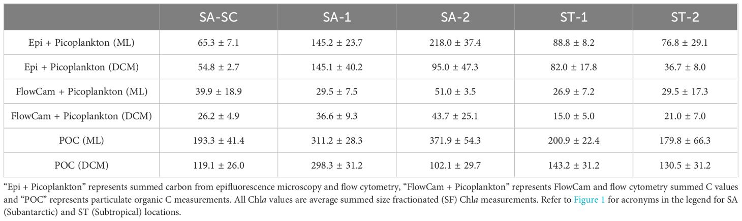
Table 2. Total C:Chla (mean ± 1 standard error) averaged across all days for each Lagrangian cycle in SA and ST areas, divided into mixed layer (ML) and deep chlorophyll maximum (DCM) horizons.

Another important methodological issue to consider is the difference between FlowCam or epi and size fractionated Chla approximation of cell size. In FlowCam and epi, we used ESD as the proxy for determining cell size whereas size fractionated Chla measurements are operationally defined by the pore sizes of the filters. Given the complex shapes of many nanoplankton and microplankton taxa, these differences in approaches to size determination can add uncertainty to size-based C:Chla estimates. For instance, Landry et al. (2009) noted up to a 2-fold overestimation of picoplankton Chla by size fractionated Chla measurements as cells with flexible walls are able to squeeze through 2 µm filter pores under vacuum pressure during filtration (Psarra et al., 2005). Notably, in the SA cycles (Figure 8A), the nanoplankton C:Chla ratio was approximately 3 times lower at 12 m depth compared to micro (nanoplankton 319.6 ± 49.0; microplankton 1044.6 ± 474.1), but approximately 50% higher at 50 m (nanoplankton 219.7 ± 53.4; microplankton 141.2 ± 54.4). The observed variability in size fractionated Chla is a key factor, as highlighted by the substantial differences between the 2 µm and 20 µm size fractions at 12 m in the SA-2 cycle. Specifically, the Chla concentrations were 5 times higher in the 2 µm fraction compared to the 20 µm fraction (0.04 µg Chla versus 0.008 µg Chla), while the C biomass measurements were similar (14.8 µg C L^-1 and 17.5 µg C L^-1, respectively).

Time of sampling may also play a role in C:Chla as our Chla data was collected at approximately 02:00, during a period with no natural light. This nighttime sampling may have implications for the interpretation of C:Chla ratios due to diel variations in chlorophyll content within phytoplankton cells. Studies have shown that Chla concentrations in many species, including diatoms, can vary throughout the day, often peaking during daylight and decreasing at night (Owens et al., 1980). This diel cycle is attributed to Chla synthesis being closely linked to photosynthetic activity, which is reduced in the absence of light. Consequently, our nighttime sampling may result in elevated C:Chla ratios, as chlorophyll levels could be lower compared to daytime measurements, while carbon content should remain relatively consistent. The magnitude of diel variation in C:Chla will depend on the relationship between photosynthesis rates during the light period, overall growth rates, and the extent to which energy storage products are mobilized during darkness to support cell synthesis (Geider, 1987).

When comparing regional C:Chla, ST regions had higher summed plankton C biomass compared to SA regions, consistent with prior studies showing highest cellular plankton C concentrations in the STF region, intermediate concentrations in the ST regions and the lowest C in the SA region (Bradford-Grieve et al., 1997). When comparing these C measurements to Chla, we find that our epi C:Chla ratios are higher than other bulk phytoplankton ratios observed in this region. For example, our data suggest average C:Chla is 260.0 ± 40.5 for nanoplankton and 859.2 ± 311.9 for microplankton at 12 m. These ratios are much higher than the bulk average C:Chla recorded for this region by Bradford-Grieve et al. (1999) of 36 in the STF and 84 in SA at 10 m. However, it is important to note the limitations of Bradford-Grieve’s dataset, as their sampling was restricted to a depth of 10 meters at just two locations in the STF and two in the SA, yet it is one of the few studies conducted in the same region as ours. In contrast, our overall averaged C:Chla for picoplankton (15.8 ± 3.2) was in range to that found in the euphotic zone of the Alboran Sea in the Mediterranean where Arin (2002) found C:Chla of 15 to 59 for cells <2 µm. However our C:Chla is higher for nanoplankton and microplankton compared to this study which ranged from 24 to 57 for cells >2 µm. Laboratory studies have found lower C:Chla ranging from 26-113 for various sized plankton including cyanophytes, chlorophytes, diatoms and dinoflagellates (Yacobi and Zohary, 2010). C:Chla tends to increases with nutrient limitation (Laws and Bannister, 1980; Liefer et al., 2018), suggesting that decreases in Chla concentrations are responsible, rather than an increase in cellular C. In our study, the entire community C:Chla was 123.8 ± 18.9 overall which is higher than previous measurements in the region (Bradford-Grieve et al., 1997; Zeldis, 2002). However, higher C:Chla has been recorded (ranging from 150 to 200) in the upper euphotic zone in the Gulf of Mexico (Selph et al., 2021), while modeling studies have predicted C:Chla to be as high as 160 in the upper euphotic zone in latitudes ranging from 0° to 35° N (Taylor et al., 1997) and 200:1 in surface waters in the California Current Ecosystem (Li et al., 2010).

Light, temperature and nutrients have a combined effect on cellular C:Chla ratios, which are dynamically adjusted to optimize the physiological state of phytoplankton (MacIntyre et al., 2000). C:Chla increases linearly with increased light at a constant temperature, yet decreases exponentially with increased temperature at constant light (Geider, 1987). C:Chla is lowest at high temperature, low irradiance and nutrient replete conditions and is maximal at low temperature, high light and nutrient limiting conditions (Geider et al., 1997). In continuous culture experiments with diatoms, C:Chla was found to be low at low irradiance and nutrient limitation (Laws and Bannister, 1980). Disentangling these competing influences can be difficult, particularly in the field as nutrient limitation, including macronutrients and trace-metals, may also impact C:Chla (Taylor et al., 2015) with iron limitation reported to greatly impact C:Chla in the Southern Ocean (Strzepek et al., 2019; Ye et al., 2023) which likely underpin the higher C:Chla observed in SA cycles. A decrease in cellular Chla in cells has been linked to iron deficiency (Glover, 1977; Boyd et al., 2001; Sunda and Huntsman, 1997) and in-situ experiments in the Southern Ocean have shown that iron fertilization led to an increase in cellular Chla concentrations and a decrease in C:Chla (Gall et al., 2001).

5 Conclusion

This study focused on the structure of phytoplankton communities in the ST and SA waters east of New Zealand, highlighting the potential influence of group-specific variation in pelagic food webs and biogeochemical processes. We found that nanoplankton tend to dominate the ST region whereas picoplankton dominated the offshore SA and microplankton dominated the SA-SC region. Our normalized size spectra data assessed the dominance of small and large phytoplankton in the community composition, finding greater dominance by small cells in SA relative to ST water. We also noted depth-related variations for picoplankton with higher phytoplankton abundance and C biomass in shallower depths, particularly for small cells. Epi-based C:Chla ratios were higher in the SA compared to the ST, and showed that picoplankton consistently exhibited lower C:Chla than larger cells. Summed biomass (autotrophs + heterotrophs) comprised ~2/3 of particulate organic carbon, suggesting that non-living detritus represents approximately 1/3 of the particulate matter available for consumers. Analyzing depth-resolved phytoplankton community composition helped achieve a more accurate representation of phytoplankton biomass patterns for future food web studies as compared to many previous studies that only examine phytoplankton community composition at one or two depths. Extending surveying under various conditions can help us disentangle these competing influences on C:Chla and help us better understand the impact of plankton community composition on biogeochemical cycles in this region.

Data availability statement

The datasets presented in this study can be found in online repositories. The names of the repository/repositories and accession number(s) can be found below: https://www.bco-dmo.org/project/754878.

Author contributions

NY: Writing – original draft, Writing – review & editing. KES: Writing – review & editing. MD: Writing – review & editing. KAS: Writing – review & editing. AG: Writing – review & editing. CF: Writing – review & editing. MS: Writing – original draft, Writing – review & editing.

Funding

The author(s) declare financial support was received for the research, authorship, and/or publication of this article. This study was made possible by funding from the Ministry for Business, Innovation and Employment (MBIE) of New Zealand, NIWA Coast and Oceans Food Webs (COES) and Ocean Flows (COOF), and the Royal Society of New Zealand Marsden Fast-track award to MD, and by U.S. National Science Foundation awards OCE- 1756610 and 1756465 to MS and KES.

Acknowledgments

This manuscript would not have been possible without the support from the captain, crew and research technicians aboard the R/V Tangaroa; thank you for your hard work and dedication while out at sea. Additionally, we would like to thank and acknowledge our collaborators at NIWA – National Institute of Water and Atmospheric Research in Aotearoa-New Zealand for all their efforts and perseverance during our research cruise.

Conflict of interest

The authors declare that the research was conducted in the absence of any commercial or financial relationships that could be construed as a potential conflict of interest.

The author(s) declared that they were an editorial board member of Frontiers, at the time of submission. This had no impact on the peer review process and the final decision.

Publisher’s note

All claims expressed in this article are solely those of the authors and do not necessarily represent those of their affiliated organizations, or those of the publisher, the editors and the reviewers. Any product that may be evaluated in this article, or claim that may be made by its manufacturer, is not guaranteed or endorsed by the publisher.

Supplementary material

The Supplementary Material for this article can be found online at: https://www.frontiersin.org/articles/10.3389/fmars.2025.1465125/full#supplementary-material

Abbreviations

C, Carbon; Chla, Chlorophyll a; C:Chla, Carbon to chlorophyll a; POC, Particulate organic carbon; SA, Subantarctic water; ST, Subtropical water; STF, Subtropical Front; SC, Southland Current; hbact, Heterotrophic bacteria; Syn, Synechococcus; Pro, Prochlorococcus; peuk, Picoeukaryotes; ML, Mixed layer; DCM, Deep chlorophyll maximum; Epi, Epifluorescence microscopy; FCM, Flow Cytometry.

References

Agustí S. (1991). Allometric scaling of light absorption and scattering by phytoplankton cells. Can. J. Fish. Aquat. Sci. 48, 763–767. doi: 10.1139/f91-091

Crossref Full Text | Google Scholar

Azam F., Fenchel T., Field J., Gray J., Meyer-Reil L., Thingstad F. (1983). The ecological role of water-column microbes in the sea. Mar. Ecol. Prog. Ser. 10, 257–263. doi: 10.3354/meps010257

Crossref Full Text | Google Scholar

Banse K. (1996). Low seasonality of low concentrations of surface chlorophyll in the Subantarctic water ring: underwater irradiance, iron, or grazing? Prog. Oceanogr. 37, 241–291. doi: 10.1016/S0079-6611(96)00006-7

Crossref Full Text | Google Scholar

Behrens E., Hogg A. M., England M. H., Bostock H. (2021). Seasonal and interannual variability of the subtropical front in the New Zealand region. J. Geophys. Res. Oceans 126, 1–25. doi: 10.1029/2020JC016412

Crossref Full Text | Google Scholar

Bertilsson S., Berglund O., Karl D. M., Chisholm S. W. (2003). Elemental composition of marine Prochlorococcus and Synechococcus : Implications for the ecological stoichiometry of the sea. Limnol. Oceanogr. 48, 1721–1731. doi: 10.4319/lo.2003.48.5.1721

Crossref Full Text | Google Scholar

Boyd P. W., Crossley A. C., DiTullio G. R., Griffiths F. B., Hutchins D. A., Queguiner B., et al. (2001). Control of phytoplankton growth by iron supply and irradiance in the subantarctic Southern Ocean: Experimental results from the SAZ Project. J. Geophys. Res. Oceans 106, 31573–31583. doi: 10.1029/2000JC000348

Crossref Full Text | Google Scholar

Boyd P. W., Strzepek R., Fu F., Hutchins D. A. (2010). Environmental control of open-ocean phytoplankton groups: Now and in the future. Limnol. Oceanogr. 55, 1353–1376. doi: 10.4319/lo.2010.55.3.1353

Crossref Full Text | Google Scholar

Bradford-Grieve J. M., Boyd P. W., Chang F. H., Chiswell S., Hadfield M., Hall J. A., et al. (1999). Pelagic ecosystem structure and functioning in the subtropical front region east of New Zealand in austral winter and spring 1993. J. Plankton Res. 21, 405–428. doi: 10.1093/plankt/21.3.405

Crossref Full Text | Google Scholar

Bradford-Grieve J. M., Chang F. H., Gall M., Pickmere S., Richards F. (1997). Size-fractionated phytoplankton standing stocks and primary production during austral winter and spring 1993 in the Subtropical Convergence region near New Zealand. N. Z. J. Mar. Freshw. Res. 31, 201–224. doi: 10.1080/00288330.1997.9516759

Crossref Full Text | Google Scholar

Bradford-Grieve J., Murdoch R., James M., Oliver M., McLeod J. (1998). Mesozooplankton biomass, composition, and potential grazing pressure on phytoplankton during austral winter and spring 1993 in the subtropical convergence region near New Zealand. Deep Sea Res. Part Oceanogr. Res. Pap. 45, 1709–1737. doi: 10.1016/S0967-0637(98)00039-9

Crossref Full Text | Google Scholar

Buesseler K. O. (1998). The decoupling of production and particulate export in the surface ocean. Glob. Biogeochem. Cycles 12, 297–310. doi: 10.1029/97GB03366

Crossref Full Text | Google Scholar

Buitenhuis E. T., Li W. K. W., Vaulot D., Lomas M. W., Landry M. R., Partensky F., et al. (2012). Picophytoplankton biomass distribution in the global ocean 10, 554–577. doi: 10.5194/essdd-5-221-2012

Crossref Full Text | Google Scholar

Calbet A., Landry M. R. (2004). Phytoplankton growth, microzooplankton grazing, and carbon cycling in marine systems. Limnol. Oceanogr. 49, 51–57. doi: 10.4319/lo.2004.49.1.0051

Crossref Full Text | Google Scholar

Carvalho F., Fitzsimmons J. N., Couto N., Waite N., Gorbunov M., Kohut J., et al. (2020). Testing the Canyon Hypothesis: Evaluating light and nutrient controls of phytoplankton growth in penguin foraging hotspots along the West Antarctic Peninsula. Limnol. Oceanogr. 65, 455–470. doi: 10.1002/lno.11313

Crossref Full Text | Google Scholar

Cassar N., Wright S. W., Thomson P. G., Trull T. W., Westwood K. J., de Salas M., et al. (2015). The relation of mixed-layer net community production to phytoplankton community composition in the Southern Ocean. Glob. Biogeochem. Cycles 29, 446–462. doi: 10.1002/2014GB004936

Crossref Full Text | Google Scholar

Chang F. H., Gall M. (1998). Phytoplankton assemblages and photosynthetic pigments during winter and spring in the Subtropical Convergence region near New Zealand. N. Z. J. Mar. Freshw. Res. 32, 515–530. doi: 10.1080/00288330.1998.9516840

Crossref Full Text | Google Scholar

Chen B., Liu H. (2010). Relationships between phytoplankton growth and cell size in surface oceans: Interactive effects of temperature, nutrients, and grazing. Limnol. Oceanogr. 55, 965–972. doi: 10.4319/lo.2010.55.3.0965

Crossref Full Text | Google Scholar

Chiswell S. M., Bostock H. C., Sutton P. J., Williams M. J. (2015). Physical oceanography of the deep seas around New Zealand: a review. N. Z. J. Mar. Freshw. Res. 49, 286–317. doi: 10.1080/00288330.2014.992918

Crossref Full Text | Google Scholar

Chiswell S. M., Safi K. A., Sander S. G., Strzepek R., Ellwood M. J., Milne A., et al. (2019). Exploring mechanisms for spring bloom evolution: contrasting 2008 and 2012 blooms in the southwest Pacific Ocean. J. Plankton Res. 41, 329–348. doi: 10.1093/plankt/fbz017

Crossref Full Text | Google Scholar

Chow A. T., Guo F., Gao S., Breuer R., Dahlgren R. A. (2005). Filter pore size selection for characterizing dissolved organic carbon and trihalomethane precursors from soils. Water Res. 39, 1255–1264. doi: 10.1016/j.watres.2005.01.004

PubMed Abstract | Crossref Full Text | Google Scholar

Claustre H. (2005). Toward a taxon-specific parameterization of bio-optical models of primary production: A case study in the North Atlantic. J. Geophys. Res. 110, C07S12. doi: 10.1029/2004JC002634

Crossref Full Text | Google Scholar

Cloern J. E. (2018). Why large cells dominate estuarine phytoplankton: Large cells dominate in estuaries. Limnol. Oceanogr. 63, S392–S409. doi: 10.1002/lno.10749

Crossref Full Text | Google Scholar

Currie K. I., Hunter K. A. (1998). Surface water carbon dioxide in the waters associated with the subtropical convergence, east of New Zealand. Deep Sea Res. Part Oceanogr. Res. Pap. 45, 1765–1777. doi: 10.1016/S0967-0637(98)00041-7

Crossref Full Text | Google Scholar

Décima M., Stukel M. R., Nodder S. D., Gutiérrez-Rodríguez A., Selph K. E., dos Santos A. L., et al. (2023). Salp blooms drive strong increases in passive carbon export in the Southern Ocean. Nat. Commun. 14, 425. doi: 10.1038/s41467-022-35204-6

PubMed Abstract | Crossref Full Text | Google Scholar

Delizo L., Smith W. O., Hall J. (2007). Taxonomic composition and growth rates of phytoplankton assemblages at the Subtropical Convergence east of New Zealand. J. Plankton Res. 29, 655–670. doi: 10.1093/plankt/fbm047

Crossref Full Text | Google Scholar

Doolittle D. F., Li W. K. W., Wood A. M. (2008). Wintertime abundance of picoplankton in the Atlantic sector of the Southern Ocean. Nova Hedwig. 133, 147–160.

Google Scholar

Dubreuil C., Denis M., Conan P., Roy S. (2003). Spatial-temporal variability of ultraplankton vertical distribution in the Antarctic frontal zones within 60–66°E, 43–46°S. Polar Biol. 26, 734–745. doi: 10.1007/s00300-003-0545-5

Crossref Full Text | Google Scholar

Dunne J. P., Armstrong R. A., Gnanadesikan A., Sarmiento J. L. (2005). Empirical and mechanistic models for the particle export ratio: MODELING THE PARTICLE EXPORT RATIO. Glob. Biogeochem. Cycles 19, 1–16. doi: 10.1029/2004GB002390

Crossref Full Text | Google Scholar

Ellwood M. J., Law C. S., Hall J., Woodward E. M. S., Strzepek R., Kuparinen J., et al. (2013). Relationships between nutrient stocks and inventories and phytoplankton physiological status along an oligotrophic meridional transect in the Tasman Sea. Deep Sea Res. Part Oceanogr. Res. Pap. 72, 102–120. doi: 10.1016/j.dsr.2012.11.001

Crossref Full Text | Google Scholar

Fender C. K., Décima M., Gutiérrez-Rodríguez A., Selph K. E., Yingling N., Stukel M. R. (2023). Prey size spectra and predator to prey size ratios of southern ocean salps. Mar. Biol. 170, 40. doi: 10.1007/s00227-023-04187-3

Crossref Full Text | Google Scholar

Finkel Z. V. (2001). Light absorption and size scaling of light-limited metabolism in marine diatoms. Limnol. Oceanogr. 46, 86–94. doi: 10.4319/lo.2001.46.1.0086

Crossref Full Text | Google Scholar

Finkel Z. V., Beardall J., Flynn K. J., Quigg A., Rees T. A. V., Raven J. A. (2010). Phytoplankton in a changing world: cell size and elemental stoichiometry. J. Plankton Res. 32, 119–137. doi: 10.1093/plankt/fbp098

Crossref Full Text | Google Scholar

Gall M. P., Boyd P. W., Hall J., Safi K. A., Chang H. (2001). Phytoplankton processes. Part 1: Community structure during the Southern Ocean Iron RElease Experiment (SOIREE). Deep Sea Res. Part II Top. Stud. Oceanogr. 48, 2551–2570. doi: 10.1016/S0967-0645(01)00008-X

Crossref Full Text | Google Scholar

Gall M., Hawes I., Boyd P. (1999). Predicting rates of primary production in the vicinity of the Subtropical Convergence east of New Zealand. N. Z. J. Mar. Freshw. Res. 33, 443–455. doi: 10.1080/00288330.1999.9516890

Crossref Full Text | Google Scholar

Garrison D. L., Gowing M. M., Hughes M. P., Campbell L., Caron D. A., Dennett M. R., et al. (2000). Microbial food web structure in the Arabian Sea: a US JGOFS study. Deep Sea Res. Part II Top. Stud. Oceanogr. 47, 1387–1422. doi: 10.1016/S0967-0645(99)00148-4

Crossref Full Text | Google Scholar

Geider R. J. (1987). Light and temperature dependence of the carbon to chlorophyll a ratio in microalgae and cyanobacteria: implications for physiology and growth of phytoplankton. New Phytol. 106, 1–34. doi: 10.1111/j.1469-8137.1987.tb04788.x

Crossref Full Text | Google Scholar

Geider R., MacIntyre H., Kana T. (1997). Dynamic model of phytoplankton growth and acclimation:responses of the balanced growth rate and the chlorophyll a:carbon ratio to light, nutrient-limitation and temperature. Mar. Ecol. Prog. Ser. 148, 187–200. doi: 10.3354/meps148187

Crossref Full Text | Google Scholar

Glover H. (1977). Effects of iron deficiency on isochrysis galbana (chrysophyceae) and phaeodactylum tricornutum (bacillariophyceae) ¹. J. Phycol. 13, 208–212. doi: 10.1111/j.1529-8817.1977.tb02917.x

Crossref Full Text | Google Scholar

Gorbunov M. Y., Falkowski P. G. (2021). Using chlorophyll fluorescence kinetics to determine photosynthesis in aquatic ecosystems. Limnol. Oceanogr. 66, 1–13. doi: 10.1002/lno.11581

Crossref Full Text | Google Scholar

Guidi L., Stemmann L., Jackson G. A., Ibanez F., Claustre H., Legendre L., et al. (2009). Effects of phytoplankton community on production, size, and export of large aggregates: A world-ocean analysis. Limnol. Oceanogr. 54, 1951–1963. doi: 10.4319/lo.2009.54.6.1951

Crossref Full Text | Google Scholar

Gutiérrez-Rodríguez A., dos Santos A. L., Safi K., Probert I., Not F., Fernández D., et al. (2022). Planktonic protist diversity across contrasting Subtropical and Subantarctic waters of the southwest Pacific. Prog. Oceanogr. 206. doi: 10.1016/j.pocean.2022.102809

Crossref Full Text | Google Scholar

Gutiérrez-Rodríguez A., Safi K., Fernández D., Forcén-Vázquez A., Gourvil P., Hoffmann L., et al. (2020). Decoupling between phytoplankton growth and microzooplankton grazing enhances productivity in subantarctic waters on Campbell Plateau, Southeast of New Zealand. J. Geophys. Res. Oceans 125, 1–28. doi: 10.1029/2019JC015550

Crossref Full Text | Google Scholar

Hall J., James M., Bradford-Grieve J. (1999). Structure and dynamics of the pelagic microbial food web of the Subtropical Convergence region east of New Zealand. Aquat. Microb. Ecol. 20, 95–105. doi: 10.3354/ame020095

Crossref Full Text | Google Scholar

James M. R., Hall J. A. (1998). Microzooplankton grazing in different water masses associated with the subtropical convergence round the south island, New Zealand. Deep Sea Res. Part Oceanogr. Res. Pap. 45, 1689–1707. doi: 10.1016/S0967-0637(98)00038-7

Crossref Full Text | Google Scholar

Key T., McCarthy A., Campbell D. A., Six C., Roy S., Finkel Z. V. (2010). Cell size trade-offs govern light exploitation strategies in marine phytoplankton. Environ. Microbiol. 12, 95–104. doi: 10.1111/j.1462-2920.2009.02046.x

PubMed Abstract | Crossref Full Text | Google Scholar

Kopczynska E. E., Dehairs F., Elskens M., Wright S. (2001). Phytoplankton and microzooplankton variability between the Subtropical and Polar Fronts south of Australia: Thriving under regenerative and new production in late summer. 13, 31597–31609. doi: 10.1029/2000JC000278

Crossref Full Text | Google Scholar

Landry M. R., Ohman M. D., Goericke R., Stukel M. R., Tsyrklevich K. (2009). Lagrangian studies of phytoplankton growth and grazing relationships in a coastal upwelling ecosystem off Southern California. Prog. Oceanogr. 83, 208–216. doi: 10.1016/j.pocean.2009.07.026

Crossref Full Text | Google Scholar

Law C. S., Smith M. J., Stevens C. L., Abraham E. R., Ellwood M. J., Hill P., et al. (2011). Did dilution limit the phytoplankton response to iron addition in HNLCLSi sub-Antarctic waters during the SAGE experiment? Deep Sea Res. Part II Top. Stud. Oceanogr. 58, 786–799. doi: 10.1016/j.dsr2.2010.10.018

Crossref Full Text | Google Scholar

Laws E. A., Bannister T. T. (1980). Nutrient- and light-limited growth of Thalassiosira fluviatilis in continuous culture, with implications for phytoplankton growth in the ocean1: Studies of T. fluviatilis. Limnol. Oceanogr. 25, 457–473. doi: 10.4319/lo.1980.25.3.0457

Crossref Full Text | Google Scholar

Legendre L., Le Fèvre J. (1995). Microbial food webs and the export of biogenic carbon in oceans. Aquat. Microb. Ecol. 9, 69–77. doi: 10.3354/ame009069

Crossref Full Text | Google Scholar

Levitus S. (1982). Climatological atlas of the world ocean. (US Department of Commerce, National Oceanic and Atmospheric Administration). Available online at: https://books.google.com/books?hl=en&lr=&id=_x0IAQAAIAAJ&oi=fnd&pg=PR14&dq=Levitus,+S.+(1982),+Climatological+atlas+of+the+world+ocean,+NOAA+Prof.+Pap.+13,+173+pp.,+U.S.+Govt.+Printing+Off.,+Washington,+D.+C.+&ots=x0KZcbn8iX&sig=nhuEF1r678-CxHrmq1ItSNSOLNk (Accessed November 22, 2024).

Google Scholar

Li W. K. W. (2002). Macroecological patterns of phytoplankton in the northwestern North Atlantic Ocean. Nature 419, 154–157. doi: 10.1038/nature00994

PubMed Abstract | Crossref Full Text | Google Scholar

Li Q. P., Franks P. J. S., Landry M. R., Goericke R., Taylor A. G. (2010). Modeling phytoplankton growth rates and chlorophyll to carbon ratios in California coastal and pelagic ecosystems. J. Geophys. Res. 115, G04003. doi: 10.1029/2009JG001111

Crossref Full Text | Google Scholar

Li X., Zhang J., Lee J. H. W. (2004). Modelling particle size distribution dynamics in marine waters. Water Res. 38, 1305–1317. doi: 10.1016/j.watres.2003.11.010

PubMed Abstract | Crossref Full Text | Google Scholar

Liefer J. D., Garg A., Campbell D. A., Irwin A. J., Finkel Z. V. (2018). Nitrogen starvation induces distinct photosynthetic responses and recovery dynamics in diatoms and prasinophytes. PLoS One 13, e0195705. doi: 10.1371/journal.pone.0195705

PubMed Abstract | Crossref Full Text | Google Scholar

MacIntyre H. L., Kana T. M., Geider R. J. (2000). The effect of water motion on short-term rates of photosynthesis by marine phytoplankton. Trends Plant Sci. 5, 12–17. doi: 10.1016/S1360-1385(99)01504-6

PubMed Abstract | Crossref Full Text | Google Scholar

Marañón E. (2009). “Phytoplankton size structure,” in Encyclopedia of ocean sciences (The Netherlands: Academic Press, Amsterdam), 445–452.

Google Scholar

Margalef R. (1978). Life-forms of phytoplankton as survival alternatives in an unstable environment. Oceanol. Acta 1, 493–509.

Google Scholar

McQuatters-Gollop A., Reid P. C., Edwards M., Burkill P. H., Castellani C., Batten S., et al. (2011). Is there a decline in marine phytoplankton? Nature 472, E6–E7. doi: 10.1038/nature09950

PubMed Abstract | Crossref Full Text | Google Scholar

Menden-Deuer S., Lessard E. J. (2000). Carbon to volume relationships for dinoflagellates, diatoms, and other protist plankton. Limnol. Oceanogr. 45, 569–579. doi: 10.4319/lo.2000.45.3.0569

Crossref Full Text | Google Scholar

Mouw C. B., Barnett A., McKinley G. A., Gloege L., Pilcher D. (2016). Phytoplankton size impact on export flux in the global ocean. Glob. Biogeochem. Cycles 30, 1542–1562. doi: 10.1002/2015GB005355

Crossref Full Text | Google Scholar

Nelson D., Dortch Q. (1996). Silicic acid depletion and silicon limitation in the plume of the Mississippi River:evidence from kinetic studies in spring and summer. Mar. Ecol. Prog. Ser. 136, 163–178. doi: 10.3354/meps136163

Crossref Full Text | Google Scholar

Nodder S. D., Duineveld G. C. A., Pilditch C. A., Sutton P. J., Probert P. K., Lavaleye M. S. S., et al. (2007). Focusing of phytodetritus deposition beneath a deep-ocean front, Chatham Rise, New Zealand. Limnol. Oceanogr. 52, 299–314. doi: 10.4319/lo.2007.52.1.0299

Crossref Full Text | Google Scholar

Owens T. G., Falkowski P. G., Whitledge T. E. (1980). Diel periodicity in cellular chlorophyll content in marine diatoms. Mar. Biol. 59, 71–77. doi: 10.1007/BF00405456

Crossref Full Text | Google Scholar

Peloquin J., Hall J., Safi K., Smith W. O., Wright S., van den Enden R. (2011). The response of phytoplankton to iron enrichment in Sub-Antarctic HNLCLSi waters: Results from the SAGE experiment. Deep Sea Res. Part II Top. Stud. Oceanogr. 58, 808–823. doi: 10.1016/j.dsr2.2010.10.021

Crossref Full Text | Google Scholar

Psarra S., Zohary T., Krom M. D., Mantoura R. F. C., Polychronaki T., Stambler N., et al. (2005). Phytoplankton response to a Lagrangian phosphate addition in the Levantine Sea (Eastern Mediterranean). Deep Sea Res. Part II Top. Stud. Oceanogr. 52, 2944–2960. doi: 10.1016/j.dsr2.2005.08.015

Crossref Full Text | Google Scholar

Rice E. W., Bridgewater L., Association A. P. H. (2012). Standard Methods for the Examination of Water and Wastewater. (Washington D.C: American Public Health Association, American Water Works Association, Water Environment Federation).

Google Scholar

Ryther J. H., Menzel D. W. (1959). Light adaptation by marine phytoplankton1. Limnol. Oceanogr. 4, 492–497. doi: 10.4319/lo.1959.4.4.0492

Crossref Full Text | Google Scholar

Safi K. A., Rodríguez A. G., Hall J. A., Pinkerton M. H. (2023). Phytoplankton dynamics, growth and microzooplankton grazing across the subtropical frontal zone, east of New Zealand. Deep Sea Res. Part II Top. Stud. Oceanogr. 208, 105271. doi: 10.1016/j.dsr2.2023.105271

Crossref Full Text | Google Scholar

Sedwick P. N., DiTullio G. R., Mackey D. J. (2000). Iron and manganese in the Ross Sea, Antarctica: Seasonal iron limitation in Antarctic shelf waters. J. Geophys. Res. Oceans 105, 11321–11336. doi: 10.1029/2000JC000256

Crossref Full Text | Google Scholar

Selph K. E. (2021). Enumeration of marine microbial organisms by flow cytometry using near-UV excitation of Hoechst 34580-stained DNA. Limnol. Oceanogr. Methods 19, 692–701. doi: 10.1002/lom3.10454

Crossref Full Text | Google Scholar

Selph K. E., Swalethorp R., Stukel M. R., Kelly T. B., Knapp A. N., Fleming K., et al. (2021). Phytoplankton community composition and biomass in the oligotrophic Gulf of Mexico. J. Plankton Res. 44, 618–637. doi: 10.1093/plankt/fbab006

Crossref Full Text | Google Scholar

Serra-Pompei C., Ward B. A., Pinti J., Visser A. W., Kiørboe T., Andersen K. H. (2022). Linking plankton size spectra and community composition to carbon export and its efficiency. Glob. Biogeochem. Cycles 36, 1–19. doi: 10.1029/2021GB007275

Crossref Full Text | Google Scholar

Sherr E. B., Sherr B. F. (1993). “Preservation and storage of samples for enumeration of heterotrophic protists.” in Handbook of methods in aquatic microbial ecology. (Boca Raton: CRC Press).

Google Scholar

Sherr E. B., Sherr B. F., Kemp P. F., Cole J. J. (Eds.) (1993). Handbook of methods in aquatic microbial ecology. (Boca Raton: Lewis Publishers).

Google Scholar

Smayda T. J. (1971). Normal and accelerated sinking of phytoplankton in the sea. Mar. Geol. 11, 105–122. doi: 10.1016/0025-3227(71)90070-3

Crossref Full Text | Google Scholar

Smith R. E. H., Kalff J. (1982). Size-Dependent phosphorus uptake kinetics and cell quota in Phytoplankton. J. Phycol. 18, 275–284. doi: 10.1111/j.1529-8817.1982.tb03184.x

Crossref Full Text | Google Scholar

Strom S. L. (2008). Microbial ecology of ocean biogeochemistry: A community perspective. Science 320, 1043–1045. doi: 10.1126/science.1153527

PubMed Abstract | Crossref Full Text | Google Scholar

Strom S. L., Macri E. L., Olson M. B. (2007). Microzooplankton grazing in the coastal Gulf of Alaska: Variations in top-down control of phytoplankton. Limnol. Oceanogr. 52, 1480–1494. doi: 10.4319/lo.2007.52.4.1480

Crossref Full Text | Google Scholar

Strzepek R. F., Boyd P. W., Sunda W. G. (2019). Photosynthetic adaptation to low iron, light, and temperature in Southern Ocean phytoplankton. Proc. Natl. Acad. Sci. 116, 4388–4393. doi: 10.1073/pnas.1810886116

PubMed Abstract | Crossref Full Text | Google Scholar

Stukel M. R., Décima M., Selph K. E., Gutiérrez-Rodríguez A. (2021). Size-specific grazing and competitive interactions between large salps and protistan grazers. Limnol. Oceanogr. 66, 2521–2534. doi: 10.1002/lno.11770

Crossref Full Text | Google Scholar

Stukel M. R., Kahru M., Benitez-Nelson C. R., Décima M., Goericke R., Landry M. R., et al. (2015). Using Lagrangian-based process studies to test satellite algorithms of vertical carbon flux in the eastern North Pacific Ocean. J. Geophys. Res. Oceans 120, 7208–7222. doi: 10.1002/2015JC011264

Crossref Full Text | Google Scholar

Sunda W. G., Huntsman S. A. (1997). Interrelated influence of iron, light and cell size on marine phytoplankton growth. Nature 390, 389–392. doi: 10.1038/37093

Crossref Full Text | Google Scholar

Sutton P. (2001). Detailed structure of the Subtropical Front over Chatham Rise, east of New Zealand. J. Geophys. Res. Oceans 106, 31045–31056. doi: 10.1029/2000JC000562

Crossref Full Text | Google Scholar

Sutton P. J. H. (2003). The Southland Current: A subantarctic current. N. Z. J. Mar. Freshw. Res. 37, 645–652. doi: 10.1080/00288330.2003.9517195

Crossref Full Text | Google Scholar

Takahashi T., Sutherland S. C., Wanninkhof R., Sweeney C., Feely R. A., Chipman D. W., et al. (2009). Climatological mean and decadal change in surface ocean pCO2, and net sea–air CO2 flux over the global oceans 27, 554–577. doi: 10.1016/j.dsr2.2008.12.009

Crossref Full Text | Google Scholar

Taylor A., Geider R., Gilbert F. (1997). Seasonal and latitudinal dependencies of phytoplankton carbon-to-chlorophyll a ratios:results of a modelling study. Mar. Ecol. Prog. Ser. 152, 51–66. doi: 10.3354/meps152051

Crossref Full Text | Google Scholar

Taylor A. G., Landry M. R., Selph K. E., Wokuluk J. J. (2015). Temporal and spatial patterns of microbial community biomass and composition in the Southern California Current Ecosystem. Deep Sea Res. Part II Top. Stud. Oceanogr. 112, 117–128. doi: 10.1016/j.dsr2.2014.02.006

Crossref Full Text | Google Scholar

Taylor A. G., Landry M. R., Selph K. E., Yang E. J. (2011). Biomass, size structure and depth distributions of the microbial community in the eastern equatorial Pacific. Deep Sea Res. Part II Top. Stud. Oceanogr. 58, 342–357. doi: 10.1016/j.dsr2.2010.08.017

Crossref Full Text | Google Scholar

Twining B. S., Nodder S. D., King A. L., Hutchins D. A., LeCleir G. R., DeBruyn J. M., et al. (2014). Differential remineralization of major and trace elements in sinking diatoms. Limnol. Oceanogr. 59, 689–704. doi: 10.4319/lo.2014.59.3.0689

Crossref Full Text | Google Scholar

Vaulot D., Courties C., Partensky F. (1989). A simple method to preserve oceanic phytoplankton for flow cytometric analyses. Cytometry 10, 629–635. doi: 10.1002/cyto.990100519

PubMed Abstract | Crossref Full Text | Google Scholar

Yacobi Y. Z., Zohary T. (2010). Carbon:chlorophyll a ratio, assimilation numbers and turnover times of Lake Kinneret phytoplankton. Hydrobiologia 639, 185–196. doi: 10.1007/s10750-009-0023-3

Crossref Full Text | Google Scholar

Yang Y., Motegi C., Yokokawa T., Nagata T. (2010). Large-scale distribution patterns of virioplankton in the upper ocean. Aquat. Microb. Ecol. 60, 233–246. doi: 10.3354/ame01428

Crossref Full Text | Google Scholar

Ye Y., Sunda W. G., Hong H., Shi D. (2023). Interrelated influence of iron, light, and CO ₂ on carbon fixation in a Southern Ocean diatom. Limnol. Oceanogr. 68, 1504–1516. doi: 10.1002/lno.12360

Crossref Full Text | Google Scholar

Zeldis J. (2002). Omnivory by copepods in the New Zealand subtropical frontal zone. J. Plankton Res. 24, 9–23. doi: 10.1093/plankt/24.1.9

Crossref Full Text | Google Scholar

Zhou M. (2006). What determines the slope of a plankton biomass spectrum? J. Plankton Res. 28, 437–448. doi: 10.1093/plankt/fbi119

Crossref Full Text | Google Scholar

Zohary T., Fishbein T., Shlichter M., Naselli-Flores L. (2017). Larger cell or colony size in winter, smaller in summer – a pattern shared by many species of Lake Kinneret phytoplankton. Inland Waters 7, 200–209. doi: 10.1080/20442041.2017.1320505

Crossref Full Text | Google Scholar