Hybrid machine learning algorithms accurately predict marine ecological communities

Predicting ecological communities is highly challenging but necessary to establish effective conservation and monitoring programs. This study aims to predict the spatial distribution of nematode associations from 25 m to 2500 m water depth over an area of 350,000 km² and understand the major oceanographic processes influencing them. The study considered data from 245 nematode genera and 44 environmental parameters from 100 stations. Data was analyzed by means of a hybrid machine learning (ML) approach, which combines unsupervised and supervised methods. The unsupervised phase detected that the nematodes were geographically structured in six associations, each with representative genera. In the supervised stage, these associations were modeled as a function of the environmental features by five supervised algorithms (Support Vector Machine, Random Forest, k-Nearest Neighbors, Naive Bayes, and Stochastic Gradient Boosting), using 80% of the samples for training, leaving the remaining for testing. Among them, the random forest was the best model with an accuracy of 86.4% in the test portion. The Random Forest (RF) model recognized 8 environmental features as significant in predicting the associations. Depth, the concentration of dissolved oxygen in the water near the bottom, the quality and quantity of phytodetritus, the proportion of coarse sand and carbonate, the sediment skewness, pH, and redox potential were the most important features structuring them. The inference of each association across the whole study area was based on the modeling results of the 8 significant environmental features. This model still correctly classified 90% of test data. Such findings demonstrated that it is possible to infer the spatial distribution of the nematode associations using only a small set of environmental features. The recommendation is thus to permanently monitor these environmental variables and run the ML models. Implementing ML approaches in monitoring programs of benthic systems will increase our prediction capacity, reduce monitoring costs, and, ultimately, support the conservation of marine systems.

1 Introduction

Monitoring and predicting the state of marine ecosystems are essential for baseline studies, management actions, and conservation programs (Nichols and Williams, 2006). Assessing the state of ecosystems requires knowing the biological communities, their variability in space and time, and their response to environmental changes. Nevertheless, modeling the species composition of communities is still a challenge. It has been traditionally done based on classical statistical methods, such as canonical and redundancy analysis, which frequently return a low proportion of the explained variance (Makarenkov and Legendre, 2002; Vieira et al., 2019) and whose predictions are rarely explored. Part of this limitation is related to model assumptions and the nature of the data, such as a large number of zeros, unbalanced designs, multi-normal distribution, and missing data (Xu and Jackson, 2019). Machine learning (ML) modeling handles some of these limitations (Olden et al., 2008; Fonseca and Vieira, 2023). Furthermore, the principle of ML is to evaluate the model’s predictive performance, a desirable aspect in the context of monitoring programs to anticipate undesirable environmental changes (Schuwirth et al., 2019).

There are various ML techniques with different degrees of learning complexity (Joshi, 2020). Each approach must be used considering the nature of the data and the problem itself (Zhou, 2012; Stupariu et al., 2022). In some specific tasks, to enhance model performance, a combination of complementary ML algorithms is performed in a sequence of analytical steps, commonly termed hybrid models (Ippolito et al., 2020; Bastille-Rousseau and Wittemyer, 2021; Kruk et al., 2022; He et al., 2023). A common approach among them is to reduce the dimensionality of a multivariate dataset based on an unsupervised learning method and then use the obtained groups as the response variable in a supervised learning method (Krueger et al., 2020; Carcillo et al., 2021; Pinto et al., 2021). In community ecology, such a two-phase hybrid approach could be useful. The first phase would consist of detecting distinct taxonomic groups, a common practice among ecologists (Clarke et al., 2014), followed by a supervised learning phase where the environmental data are used to predict the occurrence of the groups.

For oceanographic studies, ML holds promise (Rubbens et al., 2023). Environmental data like bathymetry, temperature, and surface primary productivity are obtained in high spatial-temporal resolution with sonars and satellite images, while biodiversity data are sparse and logistically challenging to obtain (Balmford and Gaston, 1999; Heink and Kowarik, 2010), particularly offshore. Accurate inferences of biodiversity based on environmental data are crucial for marine ecosystem monitoring and conservation (Guisan and Zimmermann, 2000; Guisan and Thuiller, 2005; Holon et al., 2018). One challenge of modeling marine biodiversity is that oceanographic processes are dynamic, differ in spatial extent, and interact with each other (Sonnewald et al., 2021). As such, while accurate predictions are needed, it is also important to extract the model features and the interactions within environmental data (Murdoch et al., 2019). It is based on the response of biological data and interactions between environmental variables that the major oceanographic processes can be understood and monitored.

The objective of this study is to predict, through a hybrid model, the spatial distribution of nematode associations from 25 m to 2500 m water depth over an area of approximately 350,000 km² along the Brazilian continental margin and understand the major oceanographic processes influencing them. Free-living marine nematodes are microscopic organisms mostly smaller than 0.5 mm that belong to the meiofauna (Giere, 2009). In marine sediments, nematodes are usually the most abundant component of the meiofauna. They are known as one of the best ecological indicators due to their ubiquitous presence in diverse ecosystems, with high abundance, diversity, and sensitivity to multiple environmental changes (Ridall and Ingels, 2021).

2 Methods

2.1 Study area and sampling design

The Santos Basin (SB) is located in the southeastern region of the Brazilian margin between the Campos Basin and Pelotas Basin. It is limited to the north by Cabo Frio High (22°S) and to the south by Florianopolis High (28.5°S). The basin occupies an area of approximately 350,000 km², bordering four Brazilian states along 271 km of the southeast coast and reaching down to 3000 m water depth in the São Paulo Plateau. The continental shelf is narrower (70 km) in the Cabo Frio region (Rio de Janeiro state, RJ) and wider off Santos city (230 km), in São Paulo state (SP), with declivity ranging from 1:600 to 1:1300 and shelf break depth varying from 120 m to 180 m (Mahiques et al., 2010).

Environmental and nematode assemblage data were obtained from sediment samples of the Santos Project – Santos Basin Environmental Characterization – by PETROBRAS/CENPES (Moreira et al., 2023). A total of 100 sampling stations were distributed in eight transects perpendicular to the coast and at 11 isobaths (25 m, 50 m, 75 m, 100 m, 150 m, 400 m, 700 m, 1000 m, 1300 m, 1900 m, and 2400 m). Twelve additional stations were sampled within the São Paulo Plateau region, between 1900 m and 2400 m, where most of the oil and gas production takes place. Sampling cruises were conducted in July 2019 at the continental slope and plateau (isobaths from 400 m to 2400 m) and in November 2019 at the continental shelf (from 25 m to 150 m).

2.2 Sampling and sample processing

Sediment samples were taken in three replicates with a spade-type box corer (0.25 m² surface area) or a modified Van Veen grab (231 L, 0.75 m² surface area), depending on the grain size of the sediment. Sampling was incomplete in stations P1 and B5, with only 2 successful replicates; in A7, H4, and G9, with only one successful replicate; and in G11 with no successful sampling. The nematode samples were taken from the larger samplers with a cylindrical corer (5 cm diameter, 10 cm high, 19.63 cm² area), and were stored and fixed with 10% buffered formalin. Samples for 38 environmental variables were obtained from the same box corer or Van Veen. The variables were related to the content of phytopigments, organic matter, and carbonates, and the granulometry of the sediment and were analyzed by other research parties. Details of the variables such abbreviation, name, analytical method, and the reference for more information are provided in the Supplementary Table S1. Additionally, six variables related to bottom water’s physicochemical properties and topographic characteristics were measured at each sampling station, totaling 44 environmental variables. More details about sampling and methodological analyses of the environmental variables are available in Moreira et al. (2023).

In the laboratory, nematodes were extracted from the sediment by density flotation technique (Somerfield et al., 2005) with Ludox TM 50 (Sigma-Aldrich) adjusted to the specific gravity of 1.18 g/cm³, repeated 3x with each sample. Organisms were then transferred to 10% formalin and stained with Rose Bengal. Nematodes were counted in a Dollfus plate and abundances were adjusted to no. individuals/10 cm². For the genus identification, 200 specimens were randomly separated to be mounted on glass slides for identification, after a diafanization process with glycerol 5% (Seinhorst, 1962; De Grisse, 1965). After mounting, nematodes were identified to genus level or family level, in case the genus could not be identified, using the Nemys database (Nemys Eds, 2023) and pertinent nematode taxonomic literature. The nematode slides were deposited in the Biological Collection “Prof. Edmundo F. Nonato” (ColBIO-IOUSP, 2023). Identification counts were adjusted to sample abundance. The abundance, Shannon evenness, and relative dominance (abundance of the most abundant genus divided by the total number of individuals) were calculated per station. After sample processing, the mean abundance data of 261 Nematoda genera from 99 samples were used for analysis.

2.3 Data preprocessing

The proposed hybrid model combined unsupervised and supervised machine learning methods (Fonseca and Vieira, 2023). A total of 27 analytical steps, which were separated into five phases, were performed in this pipeline (Figure 1). The first phase consisted of the data collection (yellow contour color in Figure 1) and the pre-processing steps (light blue rectangle in Figure 1). At this stage, imputation was used to fill in missing environmental data using a bagged tree model for each variable (as a function of all the others; Fonseca and Vieira, 2023). Also, highly correlated environmental variables were removed (cut off = 0.75), considering the largest mean absolute values of pairwise Spearman correlations (Kuhn, 2008; Supplementary Figure S1). After removing those variables, 24 features remained in the environmental data (Supplementary Figure S2). Hereafter, they are referred to as features since they have become input variables in the model. For the nematode data, a logarithm (log₁₀) transformation was applied.

Figure 1

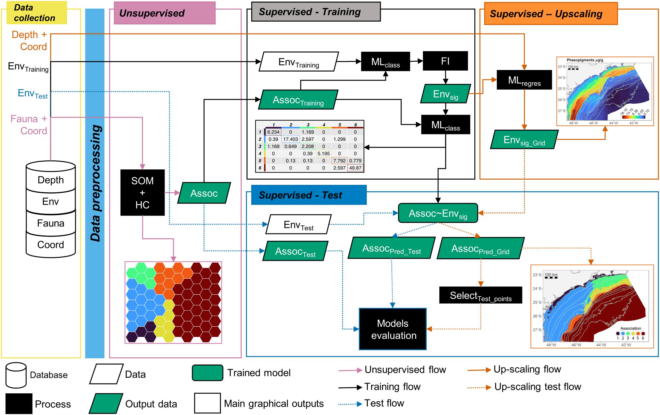
Figure 1. Analytical workflow highlighting the hybrid modeling approach implemented for the nematode assemblage data and the main outcomes. The analytical scheme is represented in five phases: Data collection, Unsupervised, Supervised-Training, Supervised Up-scaling, and Supervised-Test. Geometric forms represent the analytical processes and outputs, while the arrows represent the sequence of analytical steps. Depth, bathymetric data; Env, environmental data; Fauna, nematode genera data; Coord, coordinates data; SOM, Self Organizing Map analysis; HC, Hierarchical Clustering analysis; Assoc, taxonomic association data; ML_class, classification Machine Learning training model; FI, Feature Importance analysis; Env_sig, significant environmental features data; ML_regres, regression Machine Learning training model; Env_{sig_Grid}, significant environmental features modeled in a higher resolution grid data; Assoc~Env_sig, the trained model of the associations as function of the significant environmental features; Assoc_{Pred_*}, Associations predicted using the Env_Test (_*Test) or the Env_{Sig_Grid} (_*Grid) as predictors; Select_{Test_points}, selection of the gridded data to the points of the Test dataset.

2.4 Unsupervised phase

The second phase concerns the unsupervised analysis (light purple contour color in Figure 1), which involved a self-organizing map followed by a hierarchical clustering analysis (process box SOM + HC in Figure 1), to access and reduce the multivariate structure of the fauna into clusters (Assoc parallelogram in Figure 1). The self-organizing map (SOM) analysis is an unsupervised neural network method (Kohonen, 2001) used to aggregate similar samples into neurons, also termed map units (Best-Matching units – BMU). Here, we employed a SOM version with multiple layers (Wehrens and Buydens, 2007; Wehrens and Kruisselbrink, 2018). The dimensions of the grid was 7 x 10 neurons, with a hexagonal topology and a non-toroidal grid. The neighborhood function used was the Gaussian. The first layer was the nematode genera data with a weight of 0.95 and based on the Bray-curtis similarity index. The second layer was their respective coordinates, with a weight of 0.05 and based on the Euclidean distance. The second layer was implemented to account for potential spatial correlation between samples. For training, the complete dataset was presented 500 times to the network. Each neuron of the final map is composed of a weighted list of species termed codebook, meaning that all samples within a neuron will share the same codebook. Using the codebook provided by the SOM analysis, a hierarchical clustering (based on the Ward method with squared differences, “Ward2”) was applied to group similar BMUs and their respective samples. To choose the number of groups formed by the clustering analysis a split moving window analysis was performed to detect a discontinuity in the relation between the number of groups and the within-cluster sum of squares (WSS). The groups of neurons are referred to hereafter as taxonomic associations (Assoc, Figure 1) and used as a descriptor of the fauna. The abundance, evenness, and relative dominance of each association were compared among the associations through analysis of variance (ANOVA). The ANOVA tests were performed in R language.

2.5 Supervised training

Following the unsupervised step of the hybrid model, each taxonomic association (Assoc, Figure 1) was further used as a response variable in the Supervised Training phase (black contour color in Figure 1). This phase aims to use the best set of environmental features to model and predict those clusters through machine-learning classification algorithms. First, samples were split for validation purposes in a way that ensured a balanced partition among the associations. The training dataset (80% of the data) was used for model fitting and the test dataset (20%) for further evaluation. Then, multiple machine learning classification algorithms were performed and compared: Naïve Bayes (NB), Support Vector Machine (SVM) Learning (linear and radial), K-nearest neighbor (knn), Random Forest (RF), and Stochastic Gradient Boosting Regression Trees (sgboost). Before running the SVM and knn algorithm, the environmental features were scaled by the root mean square. All the algorithms were performed using a cross-validation method with 5 folds and 10 repetitions, and a maximum of 10 tuning combinations were chosen, except for the sgboost. For each algorithm, the highest accuracy value was used to select the optimal model among the tuning combinations. The RF models were based on 500 trees. For the sgboost models, parameter shrinkage (or learning rate) was set at 0.1 and 0.05, the minimal number of observations in the terminal nodes of the trees was 10, the number of trees was 250 and 500 and the interaction depth was performed with 1 and 2. The model with the highest accuracy and Kappa metrics was selected to be used in the following steps (process box ML_class in Figure 1).

The significant environmental features (Env_sig parallelogram in Figure 1) from the most accurate model were retrieved using a feature importance analysis (box FI in Figure 1). Except for the RF algorithm, the importance of each feature of the environmental model was obtained by random permutation of the feature/variable while the others were kept unchanged (Breiman, 2001). This process disrupts the relationship between the feature and the target variable (Assoc). Permutations were repeated 100 times, corresponding to the null normally distributed population, and the observed metric (non-permuted model) was compared to it. The statistical significance (p-value) was obtained by retrieving the proportion of extreme permuted values higher than the observed one. For the RF algorithm, the significant environmental features were obtained using the randomForestExplainer package (Jiang et al., 2020). To get a more efficient model (Assoc~Env_sig in Figure 1), only the significant environmental features (Env_sig) data were then used to train the model of the associations (Assoc_training parallelogram in Figure 1) using the same ML_class algorithm selected before. Additionally, boxplots of the environmental features were performed to understand the differences in the environmental conditions among the associations.

2.6 Supervised upscaling

Once the model Assoc~Env_sig had been trained, the next step was to predict the taxonomic associations in a 2 km x 2 km grid (orange contour color in Figure 1). To achieve this, we first modeled each significant environmental feature (Env_sig) obtained from the feature importance analysis (FI) as a function of water depth and geographical coordinates. The most accurate regression ML algorithms among the SVM Learning (linear and radial), knn, RF, and sgboost were used to build each model. The hyperparameters of the algorithms used in this phase were the same as those used in the Supervised Training phase. After running all the models, we obtained 100,555 data points for each significant environmental feature (Env_{sig_Grid} parallelogram in Figure 1). This newly created dataset was then used as predictors for the Assoc~Env_sig model (orange dotted arrows in Figure 1) to obtain the predictions of the taxonomic associations in a 2 km x 2 km grid (Assoc_{Pred_Grid} parallelogram in Figure 1).

2.7 Supervised test

To evaluate the performance of our predictions (blue contour color in Figure 1), the observed associations separated for test (Assoc_Test, Figure 1) were compared to those inferred from the environmental features from the test dataset (Assoc_{Pred_test} parallelogram in Figure 1) and those inferred from the environmental features modeled in the upscaling phase (Assoc_{Pred_Grid} parallelogram in Figure 1). Both comparisons were made based on a confusion matrix, performance metrics (accuracy and Kappa coefficient), and individual predictions at each sampling station. Based on these outcomes, it is possible to determine how much information is lost, or not, when inferring the community associations solely based on the inferences from the environmental models.

2.8 Software

All the analytical steps and outputs were done in the iMESc - An Interactive Machine Learning App for Environmental Science, which is an open-source application built on R language (Vieira et al., 2025) that can be downloaded at https://zenodo.org/record/7278042. A user guide to the application is available at https://danilocvieira.github.io/iMESc_help/#introduction. The dataset and the analysis are accessible by downloading the Savepoints at https://github.com/DaniloCVieira/imesc_savepoints and restoring them following the guide “Savepoint” at the help page of the iMESc. The selection of points from the gridded data to the points of the test data (box Select_{Test_points} in Figure 1) and the calculation of metrics between the predictions of the Test data and the gridded data (box Models evaluation in Figure 1) were made using R language. The code script can also be download at the provided link for the Savepoints. More information about the iMESc application is available in Vieira et al. (2025).

3 Results

3.1 Unsupervised phase of the hybrid model

3.1.1 Nematode associations

A total of 245 nematode genera were identified. The most abundant genera were Sabatieria, Halalaimus, Acantholaimus, and Microlaimus, representing 14.1%, 5.3%, 4.2%, and 4.2% of all individuals, respectively. The SOM analysis stabilized after a learning rate of around 0.045 for the nematode data and 0.06 for the coordinate data. The SOM network explained 75.65% of the data variance with a mean topographic error of 0.41 (Table 1). The hierarchical clustering analysis revealed that the optimal number of taxonomic associations (Assoc) was 6, with association number 6 being the most different (Figure 2A) and with more samples (Figure 2B). The spatial distribution of the associations followed a depth pattern throughout the basin and a north-south pattern on the continental shelf, where each association showed a distinct spatial extent (Figure 2D). Association 1 occurred in the shallowest region along the basin, Associations 3 and 4 occurred in the northern region of the continental shelf, while Association 2 occurred in the southern. Associations 5 and 6 were respectively restricted to the slope and plateau regions along the whole basin. The most abundant genus, Sabatieria, was dominant in Associations 2, 3, 4, and 5 (Table 2). Association 1 was characterized by higher abundances of Chomadorina, Microlaimus, Daptonema, and Sabatieria. In Association 6, Monhystrella and Acantholaimus predominated.

Table 1

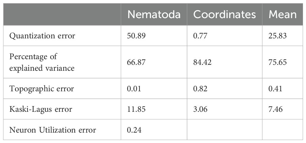
Table 1. Quality measures of the nematode and coordinate layer and the mean value of the trained SOM.

Figure 2

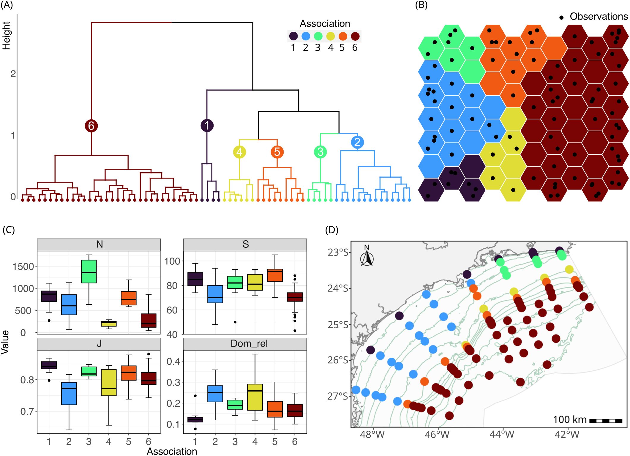
Figure 2. Nematode associations from the unsupervised phase of the hybrid model. (A) Dendrogram obtained by the hierarchical clustering of the neurons from the Self Organizing Map (SOM); (B) SOM with neurons grouped by the respective clusters; (C) box-plot of Richness, Abundance, Evenness, and Relative Dominance of each association, with the whiskers representing the minimum and maximum, the box the 25% and 75% quartiles, the line the median value and the dots the outliers; (D) map of the associations at each sampling station at the Santos Basin.

Table 2

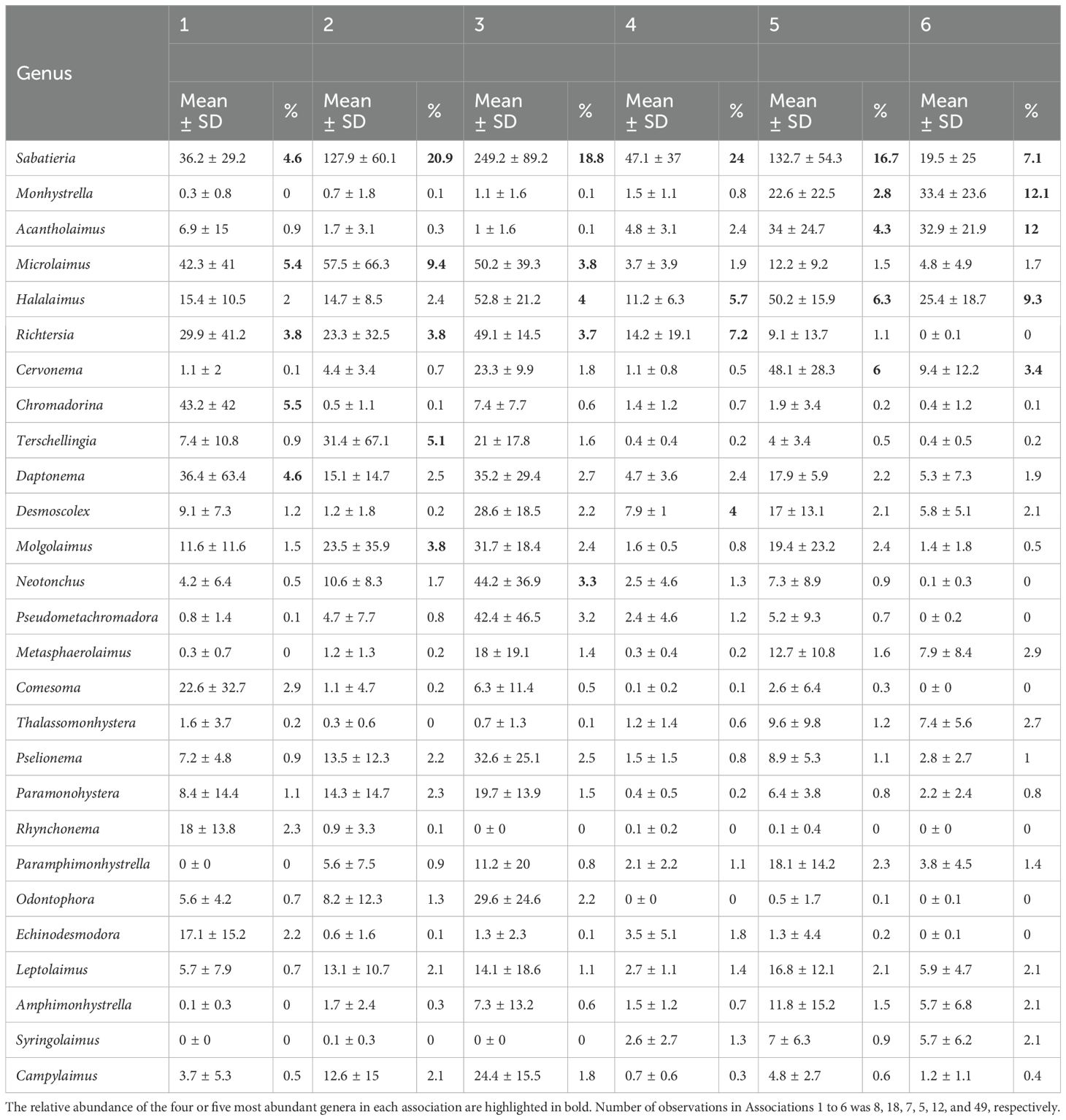
Table 2. Mean abundance, standard deviation (± SD) and relative abundance (%) of the most abundant genera (mean relative abundance >2% in at least one association) by each association.

3.1.2 Univariate descriptors of the nematode associations

Abundance per station varied from 40 to 1,758 individual/10 cm² (mean = 511 ± 392 individual/10 cm²), genus richness from 43 to 105 genera, evenness from 0.64 to 0.88 (mean value = 0.80 ± 0.04), and relative dominance from 0.07 to 0.43 (mean value = 0.18 ± 0.06). All measures varied significantly among the associations (Supplementary Table S2). Abundance was higher in Association 3, followed by Associations 1, 2, and 5, and lower in Associations 4 and 6 (Figure 2C). Associations 1 and 5 showed higher richness than Associations 2 and 6. Association 2 differed from Associations 1, 3, 5, and 6 by showing lower evenness, and Association 1 showed higher evenness than Associations 2 and 4. The relative dominance of Associations 2 and 4 was significantly higher than that of Associations 1, 5, and 6.

3.2 Nematoda associations model

The accuracy of the training models of the six ML algorithms varied from 0.80 to 0.88 and the kappa index from 0.69 to 0.83 (Table 3). The Random Forest (RF) algorithm was the most accurate and the radial Support Vector Machine (SVM radial) was the least accurate. Considering the test part of the data, the Random Forest (RF) showed the best performance, with an accuracy of 0.91 and a Kappa index of 0.88 (Table 3), and was selected as the best model (ML_class) to be used in the following steps of the analytical workflow. Among the 24 environmental features, eight were significant (significance level = 0.05; Figure 3A) selected by the RF model. Among them, water column depth (Depth) was the most important feature with a mean minimal depth of 1.29, followed in decreasing order by the Chlorophyll-a/Phaeopigments ratio (Chloa_Phaeo), sediment redox potential (Redox), content of carbonates (Carbonates), angle of the slope, content of coarse sand (CSand), sediment pH, and concentration of phaeopigments (Phaeo) in the sediment. Recalculating the model based solely on those significant environmental features, the accuracy slightly raised to 0.89 (± 0.06) and the kappa index to 0.83 (± 0.09). Association 3 showed the highest error (0.45), misclassifying part of the samples as Association 1 or 2 (Figure 3B).

Table 3

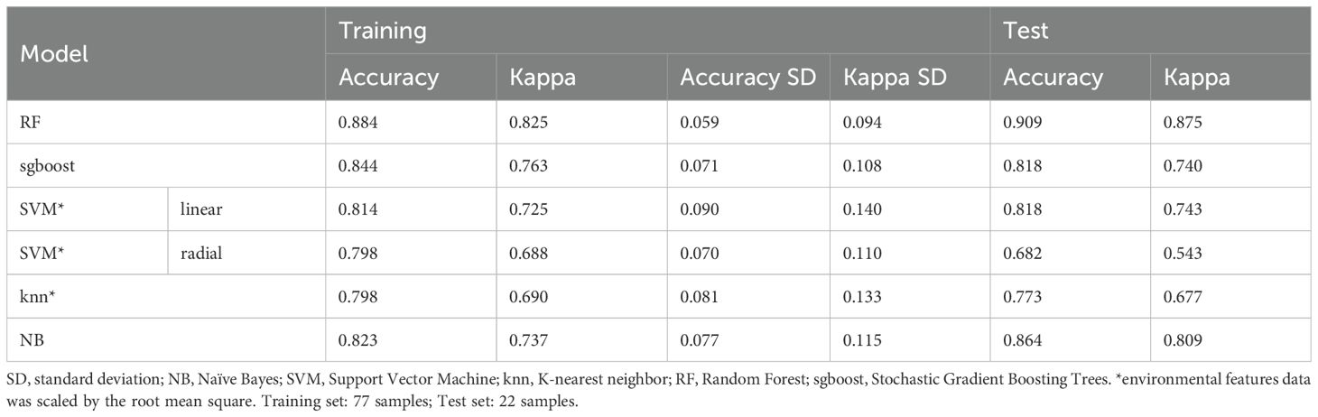
Table 3. Accuracy and Kappa index of the six models for the training and test sets.

Figure 3

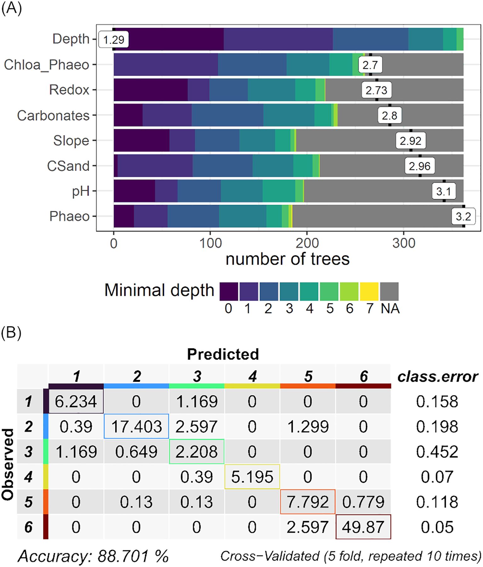
Figure 3. The Minimal Depth distribution (A) of the eight significant environmental features and (B) the confusion matrix from the training of the Random Forest model based on the significant environmental features. Depth: water column depth (m); Chloa_Phaeo: chlorophyll-a/phaeopigments ratio; Redox: sediment redox potential (mV); Carbonates: sediment content of carbonate; Slope: angle of the slope (°); CSand, sediment content of coarse sand; pH, sediment pH; Phaeo, sediment concentration of phaeopigments (µg/g).

3.3 Simulated environmental features

The accuracy of the RF models (ML_regres) of the significant environmental features (Env_sig) as a function of the depth, latitude, and longitude varied from 0.45 for coarse sand to 0.74 for carbonate (Table 4). The spatial distribution of the environmental features showed that the ocean floor of the basin was heterogeneous (Figure 4). The sediment in the northern region of the continental shelf showed a higher content of coarse sand (Figure 4F). In this region, samples were classified as Associations 1 and 3 (Figure 2D) and were characterized by coarser sediment (Supplementary Figure S3D). The concentration of phaeopigments was higher on the continental shelf, with maximum values around the isobaths of 75 m and 100 m (Figure 4H). Samples of those isobaths were classified as Association 2 in the south and Association 3 in the north (Figure 2D), and presented the highest concentration of phaeopigments in the sediment (Supplementary Figure S3F). However, values were slightly higher in the shelf southern region, reflecting a lower proportion of fresh phytopigments, compared to the north, the slope, and the plateau (Figure 4B, Supplementary Figure S3A). The carbonate content was lower near the coast and increased towards the deep, though marked by a high peak around the 150 m isobath (Figure 4D). This peak matches the location of samples from Association 4 (Figure 2D), which exhibited a high carbonate content in the sediment (Supplementary Figure S3C). Both the redox potential and the pH of the sediment revealed an evident difference between the continental shelf and the slope and plateau, with lower values in the first region (Figures 4C, H).

Table 4

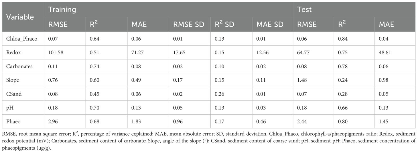
Table 4. Results of the regression RF models of the significant environmental features (Env_sig) in predicting the nematode associations.

Figure 4

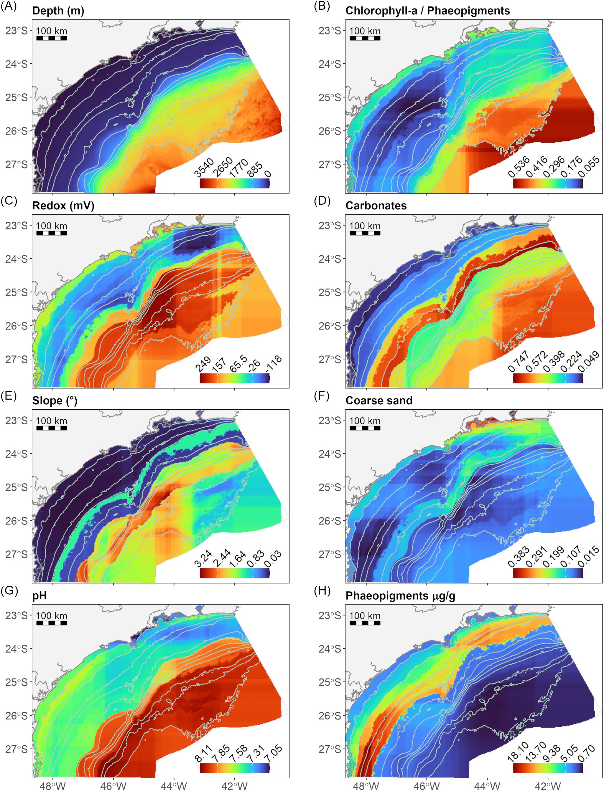
Figure 4. Spatial distribution maps of the significant environmental features (Env_sig) in predicting the nematode associations. Values plotted in the maps are the predictions of the random forest models of the environmental features as a function of depth and geographical coordinates in a 2 km x 2 km grid. (A) Depth: water column depth (m); (B) Chlorophyll-a/Phaeopigments ratio; (C) Redox: sediment redox potential (mV); (D) Carbonates: sediment content of carbonate; (E) Slope: angle of the slope (°);(F) Coarse Sand: sediment content of coarse sand grain fraction; (G) pH: sediment pH; (H) Phaeopigments: sediment concentration of phaeopigments (µg/g).

3.4 Association predictions and model validations

The results of the model of the associations (Assoc~Env_sig) using the simulated significant environmental features in the 2 km x 2 km resolution grid (Env_{sig_Grid}) evidenced the depth-related arrangement of the taxonomic associations (Figure 5A) and the difference along the continental shelf between the South and North. Association 1 occupied the shallowest region, restricted by the 25 m isobath, along the entire basin. The continental shelf was occupied by Association 2 in the southern region and Associations 3 and 4 in the northern region. Association 5 occurred along the whole basin in a narrow band on the upper slope, around the 400 m isobath. Finally, Association 6 occupied the deeper region of the basin, from the middle slope to the plateau.

Figure 5

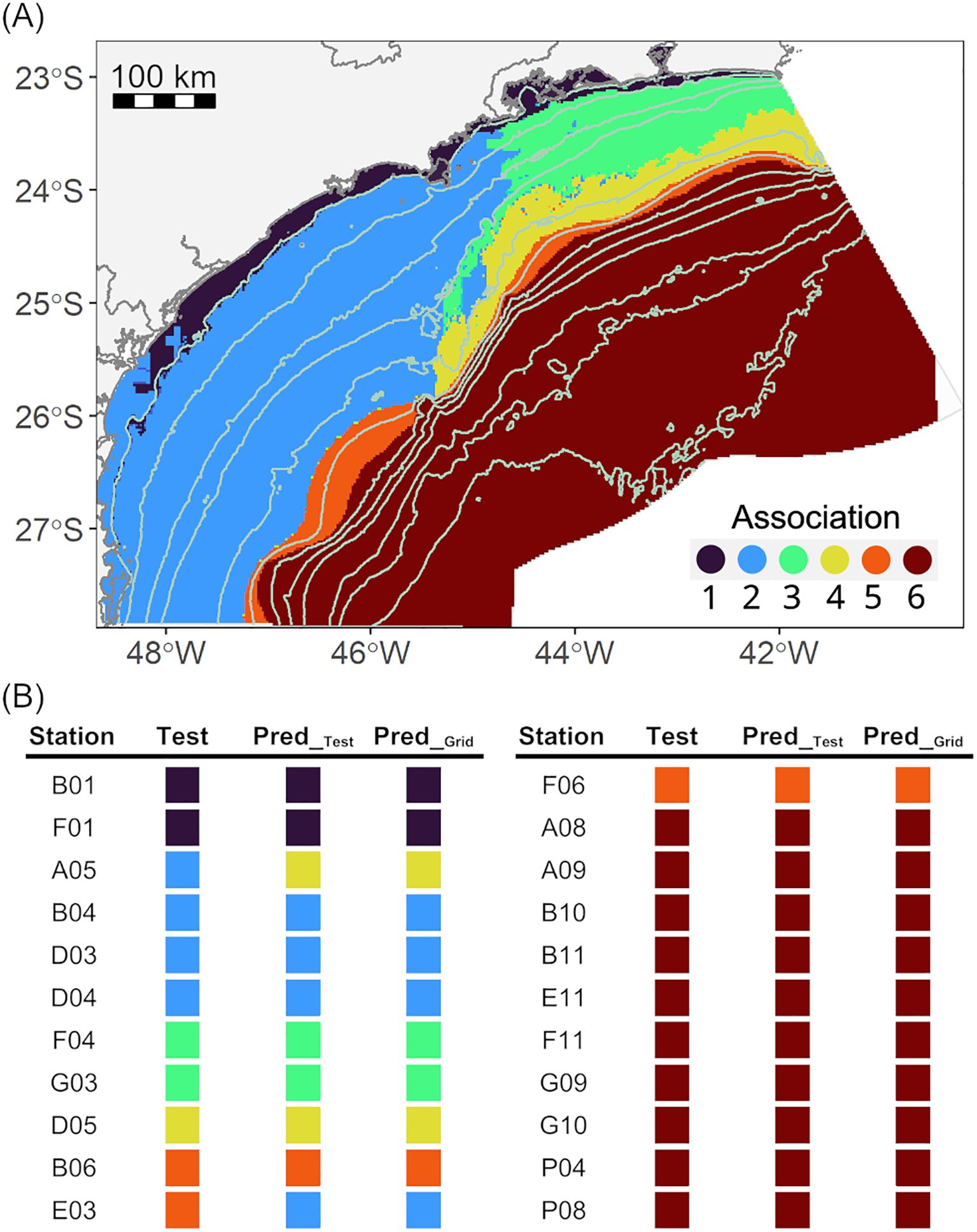
Figure 5. (A) Predicted spatial distribution map of the nematode associations of the hybrid model: values plotted in the maps are the predictions of the six associations as a function of the simulated environmental features on a bathymetric grid of 2 km x 2 km (Assoc_{Pred_Grid} in Figure 1); (B) Observed (Test) and predicted (Pred__Test, Pred__Grid) associations of the test samples: Pred__Test was predicted using the environmental features from the test dataset as predictors and Pred__Grid using the simulated environmental features in a 2 km x 2 km grid.

Comparing the observed association of the test dataset (Assoc_Test in Figure 1) with the predictions of the supervised model based on the unseen environmental features (Assoc_{Pred_Test} in Figure 1) and the simulated significant environmental features (Assoc_{Pred_Grid}; Figure 1) showed that both models classified all the associations of the test samples equally (Figure 5B). The total accuracy was 0.91 and the kappa index was 0.87. Specifically, both models misclassified only two of the 22 samples (Figure 5B).

4 Discussion

The proposed hybrid model predicted with 91% accuracy the spatial distribution of nematode associations as a function of a small set of important environmental features. From a theoretical standpoint, the reduction of dimensionality of the nematode data into associations, along with accurate predictions, suggests that the Basin is formed by distinct local communities, constituting a metacommunity (Wilson, 1992; Leibold et al., 2004). As shown by the feature importance analysis, these local communities are probably structured by depth, supply of potential food sources, such as Chlorophyll-a and Phaeopigments, topography, and the properties of the sediments, as well as other environmental variables that were highly correlated with them (Supplementary Figure S1).

Although depth is a key variable in predicting nematode associations, it is not, per se, an environmental driver of community structure; instead, it is a geographical variable that reflects a strong environmental gradient. Towards the deep, as we move away from the continental sources of sediments and organic matter and into less energetic environments, the granulometric characteristics of the sediment change, as well as its physicochemical properties and food availability (Suess, 1980; Mahiques et al., 1999; Restreppo et al., 2020). Along the Santos Basin, this was not different. On the continental shelf, sediment was coarser, with lower redox and pH values, and a higher contribution of fresher organic matter (Carreira et al., 2023; Figueiredo Jr. et al., 2023). On the other hand, muddy sediments extended over the slope and plateau, where the organic matter was scarcer and less fresh (Carreira et al., 2023; Figueiredo et al., 2023). The contrasting environmental conditions between the continental shelf and slope were also reflected in the fauna. The food-rich conditions of the continental shelf supported higher abundances of nematodes, as observed for Associations 1, 2, and 3 in contrast to Associations 4 and 6. The differences are also present in the taxonomic composition. For instance, Associations 1, 2, and 3 showed a greater abundance of typical genera from continental shelves worldwide, like Sabatiera, Microlaimus, and Daptonema (Muthumbi et al., 2004; Vanreusel et al., 2010; Muthumbi et al., 2011). In contrast, Association 6 was dominated by Acantholaimus, Monhystrella, and Halalaimus, common genera from slopes and deep-sea habitats (Vanreusel et al., 2010; Macheriotou et al., 2021; Armenteros et al., 2022, 2024).

In the continental shelf, the north-south pattern was evidenced by Association 2 in the south and Associations 3 and 4 in the north. Such a pattern results from the boundary between two sedimentation zones related to different oceanographic processes (Mahiques et al., 1999). The south receives low-salinity and cold nutrient-rich waters from the Sub-Antarctic Argentinian shelf, the La Plata River runoff, and the Patos Lagoon (Piola et al., 2000; de Souza and Robinson, 2004; Brandini et al., 2018). The interaction of those waters with the meandering of the Brazil Current and the morphology of the shelf increases the productivity and sedimentation rates, resulting in the predominance of finer and homogeneous sediments with an accumulation of organic matter (Carreira et al., 2023; Mahiques et al., 2010). High organic matter inputs in sediments stimulate bacterial activity, which leads to a reduced environment (Li et al., 2022). Genera like Sabatieria, Microlaimus, and Terschellingia, which were the most abundant of Association 2, are known to dominate sediments under such conditions (Van Gaever et al., 2009; Vanreusel et al., 2010). In the northern portion of the basin, high productivity events also occur here due to the onshore motion in the mid-shelf and the coastal upwelling of the South Atlantic Central Water (SACW). It promotes the deposition of higher-quality organic matter to the bottom (Brandini et al., 2018), impacting the benthic systems (Sumida et al., 2005; De Léo and Pires-Vanin, 2006). However, sediments are coarser and more heterogeneous in this region due to the complex hydrodynamics associated with the coastline shape and narrower shelf (Mahiques et al., 1999, 2010; Figueiredo et al., 2023). Though genera like Sabatieira and Microlaimus remained abundant in Associations 3 and 4, typical genera of coarser sediment, like Richtersia, and deeper areas, like Halalaimus, become more abundant. Particularly for Association 4, characterized by carbonates from bioconstruction fields (Figueiredo et al., 2023), the abundance of Desmoscolex increased. This taxon is known for its affinity to habitats with carbonated structures (Vanreusel et al., 2010). As we go deeper, towards the slope and plateau, environments with muddy sediments and scarce organic matter dominate (Carreira et al., 2023). While Association 5 showed a transition in taxa composition between the shelf and the deeper stations, Association 6 was typical from deep seas worldwide, with low abundances and dominance of typical deep-sea genera (Vanreusel et al., 2010; Lins et al., 2017).

The results of this study improve our understanding of the spatial structure of the benthic community of the Basin. Our study provided a comprehensive analysis of the entire Santos Basin, different from studies with macrofaunal and foraminiferal communities in the same basin which were restricted to the shelf or slope and plateau areas (Araújo et al., 2023; Moura et al., 2023). As suggested by meiofauna higher taxa data, the upwelling of the South Atlantic Central Water (SACW) and the intrusion of waters from the south with the contribution of the La Plata River are the main processes structuring the benthos in the continental shelf (Gallucci et al., 2023; Moura et al., 2023). Compared with the patterns observed for the meiofauna, the present study analytically confirmed the existence of 6 benthic zones in the Basin. Both studies recognized the Lower Slope and Plateau, the Upper and Mid-Slope, and the Upwelling as unique zones. Nonetheless, while the meiofauna study separated the southern portion of the continental shelf in two, observing a tradeoff in the abundances of kinorhynch, polychaete, and copepods associated with the concentrations of phytodetritus (Gallucci et al., 2023), the nematode genera data separated a coastal area (Association 1) from the rest of the southern portion of the continental shelf (Association 2). It is suggestive that copepods, kinorhynchs, and polychaetes are more sensitive to changes in phytodetritus deposition (Landers et al., 2020; Pruski et al., 2021), while nematodes to changes in granulometric properties of the sediment. The differences in responses between nematodes and other meiofauna taxa have already been reported (e.g. Stark et al., 2020). Such findings demonstrate the importance of monitoring multiple ecological indicators since each may respond differently to environmental changes.

Compared to traditional analytical tools commonly applied in community ecology, our hybrid approach offers at least three advantages. The first is the possibility of making accurate predictions; the second is the selection of the essential environmental variables to make the predictions, and the third is the possibility of continuous learning with the increment of new data. Accurate predictions are essential in regions with limited data, especially regarding biodiversity data. Since human activities are constantly pressuring the systems, knowing ahead of the biodiversity of an unsampled location gives us better support for management decisions. As some data are less laborious and expensive to obtain than others, such as granulometry versus biodiversity data, selecting a set of predictors by the hybrid model permits optimizing sampling strategies, data processing, and ultimately, the efficiency of monitoring programs. Particularly for the Santos Basin, it is crucial now to include additional variability, such as temporal variation or data from unsampled regions, to validate the model’s performance and enhance our understanding of the system. This can be done continually, allowing the model to improve with each new income (Fonseca and Vieira, 2023). The hybrid model approach can be applied to any scenario involving the simultaneous analysis of multiple species along with a set of environmental variables. By employing such a methodology, we move from the traditional hypothesis testing approach commonly applied to community ecology to a predictive modeling approach. Comprehensive baseline studies coupled with robust predictive models are the first steps toward implementing effective monitoring programs (Lindenmayer and Likens, 2010; Fonseca and Vieira, 2023). Based on them it is possible to predict the response of multiple ecological indicators to environmental changes and therefore build a roadmap for the validation of monitoring programs. This is a significant step towards the conservation of natural ecosystems.

Data availability statement

The datasets presented in this study can be found in online repositories. The names of the repository/repositories and accession number(s) can be found in the article/Supplementary Material.

Ethics statement

The manuscript presents research on animals that do not require ethical approval for their study.

Author contributions

LY: Conceptualization, Formal analysis, Investigation, Methodology, Writing – original draft, Writing – review & editing, Visualization. FG: Conceptualization, Funding acquisition, Investigation, Project administration, Resources, Supervision, Writing – review & editing. DV: Conceptualization, Formal analysis, Investigation, Methodology, Software, Visualization, Writing – review & editing. PG: Data curation, Investigation, Writing – review & editing. SB: Data curation, Investigation, Writing – review & editing. TC: Funding acquisition, Project administration, Resources, Supervision, Writing – review & editing. GF: Conceptualization, Formal analysis, Investigation, Methodology, Supervision, Writing – original draft, Writing – review & editing.

Funding

The author(s) declare that financial support was received for the research and/or publication of this article. Data used in this study were provided by the Santos Project - PCR-BS, which was funded, promoted, and executed by Petrobras. Petrobras was not involved in the analysis and interpretation of data, the writing of this article, or the decision to submit it for publication. GF receives support from CNPQ under grant number 306780/2022-4.

Acknowledgments

The authors acknowledge Petrobras for promoting and executing the Santos Project - PCR-BS, Daniel Moreira for coordinating the PCR-BS project, and Silvia Helena de Mello e Souza for coordinating the subproject “Benthos”. We would also like to thank Prof. Alberto Figueiredo, Prof. Renato Carreira, and Prof. Cízia Mara Hercos for making environmental data available. We are grateful to the members of the meiofauna team for their valuable help and commitment to sample processing and Prof. Wandrey Watanabe for his valuable physical oceanography consultancy and help with graphical items. Gustavo Fonseca acknowledges the support of CNPQ under grant number 306780/2022-4.

Conflict of interest

The authors declare that the research was conducted in the absence of any commercial or financial relationships that could be construed as a potential conflict of interest.

Publisher’s note

All claims expressed in this article are solely those of the authors and do not necessarily represent those of their affiliated organizations, or those of the publisher, the editors and the reviewers. Any product that may be evaluated in this article, or claim that may be made by its manufacturer, is not guaranteed or endorsed by the publisher.

Supplementary material

The Supplementary Material for this article can be found online at: https://www.frontiersin.org/articles/10.3389/fmars.2025.1458014/full#supplementary-material

References

Araújo B. D., Yamashita C., Santarosa A. C. A., Rocha A. V., Vicente T. M., Mendes R. N. M., et al. (2023). Deep-sea living (stained) benthic foraminifera from the continental slope and São Paulo Plateau, Santos Basin (SW Atlantic): ecological insights. Ocean Coast. Res. 71, e23025. doi: 10.1590/2675-2824071.22080bda

Crossref Full Text | Google Scholar

Armenteros M., Marzo-Pérez D., Pérez-García J. A., Schwing P. T., Ruiz-Abierno A., Díaz-Asencio M., et al. (2024). Setting an environmental baseline for the deep-sea slope offshore northwestern Cuba (Southeastern Gulf of Mexico) using sediments and nematode diversity. Thalass. Int. J. Mar. Sci 40, 931–945. doi: 10.1007/s41208-024-00691-5

Crossref Full Text | Google Scholar

Armenteros M., Quintanar-Retama O., Gracia A. (2022). Depth-related patterns and regional diversity of free-living nematodes in the deep-sea Southwestern Gulf of Mexico. Front. Mar. Sci. 9. doi: 10.3389/fmars.2022.1023996

Crossref Full Text | Google Scholar

Balmford A., Gaston K. J. (1999). Why biodiversity surveys are good value. Nature 398, 204–205. doi: 10.1038/18339

Crossref Full Text | Google Scholar

Bastille-Rousseau G., Wittemyer G. (2021). Characterizing the landscape of movement to identify critical wildlife habitat and corridors. Conserv. Biol. 35, 346–359. doi: 10.1111/cobi.13519

PubMed Abstract | Crossref Full Text | Google Scholar

Brandini F. P., Tura P. M., Santos P. P. G. M. (2018). Ecosystem responses to biogeochemical fronts in the South Brazil Bight. Prog. Oceanogr. 164, 52–62. doi: 10.1016/j.pocean.2018.04.012

Crossref Full Text | Google Scholar

Breiman L. (2001). Random forests. Mach. Learn. 45, 5–32. doi: 10.1023/A:1010933404324

Crossref Full Text | Google Scholar

Carcillo F., Le Borgne Y.-A., Caelen O., Kessaci Y., Oblé F., Bontempi G. (2021). Combining unsupervised and supervised learning in credit card fraud detection. Inf. Sci. 557, 317–331. doi: 10.1016/j.ins.2019.05.042

Crossref Full Text | Google Scholar

Carreira R. S., Lazzari L., Ceccopieri M., Rozo L., Martins D., Fonseca G., et al. (2023). Sedimentary organic matter accumulation provinces in the Santos Basin, SW Atlantic: insights from multiple bulk proxies. Ocean Coast. Res. 71, e23030. doi: 10.1590/2675-2824071.22061rsc

Crossref Full Text | Google Scholar

Clarke K. R., Gorley R. N., Somerfield P. J., Warwick R. M. (2014). Change in marine communities: an approach to statistical analysis and interpretation. 3rd ed (Plymouth: Primer-E Ltd).

Google Scholar

ColBIO-IOUSP (2023). Coleção Biológica Prof. Edmundo F. Nonato. São Paulo, Brazil: Instituto Oceanográfico da Universidade de São Paulo.

Google Scholar

De Grisse A. (1965). A labour-saving method for fixing and transferring eelworms to anhydrous glycerin. Landbouw Hogesch. OpzoekStns—Leerstoel Dierkd. Gent. 4.

Google Scholar

De Léo F. C., Pires-Vanin A. M. S. (2006). Benthic megafauna communities under the influence of the South Atlantic Central Water intrusion onto the Brazilian SE shelf: A comparison between an upwelling and a non-upwelling ecosystem. J. Mar. Syst. 60, 268–284. doi: 10.1016/j.jmarsys.2006.02.002

Crossref Full Text | Google Scholar

de Souza R. B., Robinson I. S. (2004). Lagrangian and satellite observations of the Brazilian Coastal Current. Cont. Shelf Res. 24, 241–262. doi: 10.1016/j.csr.2003.10.001

Crossref Full Text | Google Scholar

Figueiredo J. A. G., Carneiro J. C., dos Santos Filho J. R. (2023). Santos Basin continental shelf morphology, sedimentology, and slope sediment distribution. Ocean Coast. Res. 71, e23007. doi: 10.1590/2675-2824071.22064agfj

Crossref Full Text | Google Scholar

Fonseca G., Vieira D. C. (2023). Overcoming the challenges of data integration in ecosystem studies with machine learning workflows: an example from the Santos project. Ocean Coast. Res. 71, e23021. doi: 10.1590/2675-2824071.22044gf

Crossref Full Text | Google Scholar

Gallucci F., Fonseca G., Vieira D. C., Yaginuma L. E., Gheller P. F., Brito S., et al. (2023). Predicting large-scale spatial patterns of marine meiofauna: implications for environmental monitoring. Ocean Coast. Res. 71, e23037. doi: 10.1590/2675-2824071.22070fg

Crossref Full Text | Google Scholar

Giere O. (2009). Meiobenthology: The Microscopic Motile Fauna of Aquatic Sediments. 2nd ed (Berlin, Heidelberg: Springer). doi: 10.1007/978-3-540-68661-3

Crossref Full Text | Google Scholar

Guisan A., Thuiller W. (2005). Predicting species distribution: offering more than simple habitat models. Ecol. Lett. 8, 993–1009. doi: 10.1111/j.1461-0248.2005.00792.x

PubMed Abstract | Crossref Full Text | Google Scholar

Guisan A., Zimmermann N. E. (2000). Predictive habitat distribution models in ecology. Ecol. Model. 135, 147–186. doi: 10.1016/S0304-3800(00)00354-9

Crossref Full Text | Google Scholar

He B., Zhao Y., Liu S., Ahmad S., Mao W. (2023). Mapping seagrass habitats of potential suitability using a hybrid machine learning model. Front. Ecol. Evol. 11. doi: 10.3389/fevo.2023.1116083

Crossref Full Text | Google Scholar

Heink U., Kowarik I. (2010). What criteria should be used to select biodiversity indicators? Biodivers. Conserv. 19, 3769–3797. doi: 10.1007/s10531-010-9926-6

Crossref Full Text | Google Scholar

Holon F., Marre G., Parravicini V., Mouquet N., Bockel T., Descamp P., et al. (2018). A predictive model based on multiple coastal anthropogenic pressures explains the degradation status of a marine ecosystem: Implications for management and conservation. Biol. Conserv. 222, 125–135. doi: 10.1016/j.biocon.2018.04.006

Crossref Full Text | Google Scholar

Ippolito M., Ferguson J., Jenson F. (2020). Improving facies prediction by combining supervised and unsupervised learning methods. J. Pet. Sci. Eng. 200, 108300. doi: 10.1016/j.petrol.2020.108300

Crossref Full Text | Google Scholar

Jiang Y., Biecek P., Paluszyńska O., Kobylinska K. (2020). ModelOriented/randomForestExplainer: CRAN release 0.10.1 (v0.10.1). Zenodo. doi: 10.5281/zenodo.3941250

Crossref Full Text | Google Scholar

Joshi A. V. (2020). Machine Learning and Artificial Intelligence (Cham: Springer International Publishing). doi: 10.1007/978-3-030-26622-6

Crossref Full Text | Google Scholar

Kohonen T. (2001). Self-Organizing Maps, Springer Series in Information Sciences (Berlin, Heidelberg: Springer). doi: 10.1007/978-3-642-56927-2

Crossref Full Text | Google Scholar

Krueger R., Beyer J., Jang W.-D., Kim N. W., Sokolov A., Sorger P. K., et al. (2020). Facetto: combining unsupervised and supervised learning for hierarchical phenotype analysis in multi-channel image data. IEEE Trans. Vis. Comput. Graph. 26, 227–237. doi: 10.1109/TVCG.2019.2934547

PubMed Abstract | Crossref Full Text | Google Scholar

Kruk M., Goździejewska A. M., Artiemjew P. (2022). Predicting the effects of winter water warming in artificial lakes on zooplankton and its environment using combined machine learning models. Sci. Rep. 12, 16145. doi: 10.1038/s41598-022-20604-x

PubMed Abstract | Crossref Full Text | Google Scholar

Kuhn M. (2008). Building predictive models in R using the caret package. J. Stat. Software 28, 1–26. doi: 10.18637/jss.v028.i05

Crossref Full Text | Google Scholar

Landers S. C., Bassham R. D., Miller J. M., Ingels J., Sánchez N., Sørensen M. V. (2020). Kinorhynch communities from Alabama coastal waters. Mar. Biol. Res. 16, 494–504. doi: 10.1080/17451000.2020.1789660

Crossref Full Text | Google Scholar

Leibold M. A., Holyoak M., Mouquet N., Amarasekare P., Chase J. M., Hoopes M. F., et al. (2004). The metacommunity concept: a framework for multi-scale community ecology: The metacommunity concept. Ecol. Lett. 7, 601–613. doi: 10.1111/j.1461-0248.2004.00608.x

Crossref Full Text | Google Scholar

Li S., Fang J., Zhu X., Spencer R. G. M., Álvarez-Salgado X. A., Deng Y., et al. (2022). Properties of sediment dissolved organic matter respond to eutrophication and interact with bacterial communities in a plateau lake. Environ. pollut. 301, 118996. doi: 10.1016/j.envpol.2022.118996

PubMed Abstract | Crossref Full Text | Google Scholar

Lindenmayer D. B., Likens G. E. (2010). The science and application of ecological monitoring. Biol. Conserv. 143, 1317–1328. doi: 10.1016/j.biocon.2010.02.013

Crossref Full Text | Google Scholar

Lins L., Leliaert F., Riehl T., Pinto Ramalho S., Alfaro Cordova E., Morgado Esteves A., et al. (2017). Evaluating environmental drivers of spatial variability in free-living nematode assemblages along the Portuguese margin. Biogeosciences 14, 651–669. doi: 10.5194/bg-14-651-2017

Crossref Full Text | Google Scholar

Macheriotou L., Rigaux A., Olu K., Zeppilli D., Derycke S., Vanreusel A. (2021). Deep-sea nematodes of the Mozambique channel: evidence of random community assembly dynamics in seep sediments. Front. Mar. Sci. 8. doi: 10.3389/fmars.2021.549834

Crossref Full Text | Google Scholar

Mahiques M. M., Mishima Y., Rodrigues M. (1999). Characteristics of the sedimentary organic matter on the inner and middle continental shelf between Guanabara Bay and São Francisco do Sul, southeastern Brazilian margin. Cont. Shelf Res. 19, 775–798. doi: 10.1016/S0278-4343(98)00105-8

Crossref Full Text | Google Scholar

Mahiques M. M. D., Sousa S.H.D.M.E., Furtado V. V., Tessler M. G., Toledo F. A. D. L., Burone L., et al. (2010). The Southern Brazilian shelf: general characteristics, quaternary evolution and sediment distribution. Braz. J. Oceanogr. 58, 25–34. doi: 10.1590/S1679-87592010000600004

Crossref Full Text | Google Scholar

Makarenkov V., Legendre P. (2002). Nonlinear redundancy analysis and canonical correspondence analysis based on polynomial regression. Ecology 83, 1146–1161. doi: 10.1890/0012-9658(2002)083[1146:NRAACC]2.0.CO;2

Crossref Full Text | Google Scholar

Moreira D. L., Dalto A. G., Figueiredo A. G. Jr., Valerio A. M., Detoni A. M. S., Bonecker A. C. T., et al. (2023). Multidisciplinary scientific cruises for environmental characterization in the Santos Basin – methods and sampling design. Ocean Coast. Res. 71, e23022. doi: 10.1590/2675-2824071.22072dlm

Crossref Full Text | Google Scholar

Moura R. B. D., Dalto A. G., Sallorenzo I. D. A., Moreira D. L., Lavrado H. P. (2023). Community structure of the benthic macrofauna along the continental slope of Santos Basin and São Paulo plateau, SW Atlantic. Ocean Coast. Res. 71, e23032. doi: 10.1590/2675-2824071.22091rbdm

Crossref Full Text | Google Scholar

Murdoch W. J., Singh C., Kumbier K., Abbasi-Asl R., Yu B. (2019). Definitions, methods, and applications in interpretable machine learning. Proc. Natl. Acad. Sci. 116, 22071–22080. doi: 10.1073/pnas.1900654116

PubMed Abstract | Crossref Full Text | Google Scholar

Muthumbi A. W., Vanreusel A., Duineveld G., Soetaert K., Vincx M. (2004). Nematode Community Structure along the Continental Slope off the Kenyan Coast, Western Indian Ocean. Int. Rev. Hydrobiol. 89, 188–205. doi: 10.1002/iroh.200310689

Crossref Full Text | Google Scholar

Muthumbi W. A., Vanreusel A., Vincx M. (2011). Taxon-related diversity patterns from the continental shelf to the slope: a case study on nematodes from the Western Indian Ocean. Mar. Ecol.- Evol. Perspect. 32, 453–467. doi: 10.1111/j.1439-0485.2011.00449.x

Crossref Full Text | Google Scholar

Nemys Eds. (2023). Nemys: World Database of Nematodes. Available online at: https://nemys.ugent.be (Accessed August 18, 2023).

Google Scholar

Nichols J. D., Williams B. K. (2006). Monitoring for conservation. Trends Ecol. Evol. 21, 668–673. doi: 10.1016/j.tree.2006.08.007

PubMed Abstract | Crossref Full Text | Google Scholar

Olden J. D., Lawler J. J., Poff N. L. (2008). Machine learning methods without tears: A primer for ecologists. Q. Rev. Biol. 83, 171–193. doi: 10.1086/587826

PubMed Abstract | Crossref Full Text | Google Scholar

Pinto A., Pereira S., Meier R., Wiest R., Alves V., Reyes M., et al. (2021). Combining unsupervised and supervised learning for predicting the final stroke lesion. Med. Image Anal. 69, 101888. doi: 10.1016/j.media.2020.101888

PubMed Abstract | Crossref Full Text | Google Scholar

Piola A. R., Campos E. J. D., Möller J. O. O., Charo M., Martinez C. (2000). Subtropical Shelf Front off eastern South America. J. Geophys. Res. Oceans 105, 6565–6578. doi: 10.1029/1999JC000300

Crossref Full Text | Google Scholar

Pruski A. M., Rzeznik-Orignac J., Kerhervé P., Vétion G., Bourgeois S., Péru E., et al. (2021). Dynamic of organic matter and meiofaunal community on a river-dominated shelf (Rhône prodelta, NW Mediterranean Sea): Responses to river regime. Estuar. Coast. Shelf Sci. 253, 107274. doi: 10.1016/j.ecss.2021.107274

Crossref Full Text | Google Scholar

Restreppo G. A., Wood W. T., Phrampus B. J. (2020). Oceanic sediment accumulation rates predicted via machine learning algorithm: towards sediment characterization on a global scale. Geo-Mar. Lett. 40, 755–763. doi: 10.1007/s00367-020-00669-1

Crossref Full Text | Google Scholar

Ridall A., Ingels J. (2021). Suitability of free-living marine nematodes as bioindicators: status and future considerations. Front. Mar. Sci. 8. doi: 10.3389/fmars.2021.685327

Crossref Full Text | Google Scholar

Rubbens P., Brodie S., Cordier T., Destro Barcellos D., Devos P., Fernandes-Salvador J. A., et al. (2023). Machine learning in marine ecology: an overview of techniques and applications. ICES J. Mar. Sci. 80, 1829–1853. doi: 10.1093/icesjms/fsad100

Crossref Full Text | Google Scholar

Schuwirth N., Borgwardt F., Domisch S., Friedrichs M., Kattwinkel M., Kneis D., et al. (2019). How to make ecological models useful for environmental management. Ecol. Model. 411, 108784. doi: 10.1016/j.ecolmodel.2019.108784

Crossref Full Text | Google Scholar

Seinhorst J. W. (1962). Modifications of the elutriation method for extracting nematodes from soil. Nematologica 8, 117–128. doi: 10.1163/187529262X00332

Crossref Full Text | Google Scholar

Somerfield P. J., Warwick R. M., Moens T. (2005). “Meiofauna techniques,” in Methods for the Study of Marine Benthos. 3rd Edition, Eleftheriou A., McIntyre A. (Oxford: Blackwell), 229–272. doi: 10.1002/9780470995129.ch6

Crossref Full Text | Google Scholar

Sonnewald M., Lguensat R., Jones D. C., Dueben P. D., Brajard J., Balaji V. (2021). Bridging observations, theory and numerical simulation of the ocean using machine learning. Environ. Res. Lett. 16, 073008. doi: 10.1088/1748-9326/ac0eb0

Crossref Full Text | Google Scholar

Stark J. S., Mohammad M., McMinn A., Ingels J. (2020). Diversity, abundance, spatial variation, and human impacts in marine meiobenthic nematode and copepod communities at Casey Station, East Antarctica. Front. Mar. Sci. 7. doi: 10.3389/fmars.2020.00480

Crossref Full Text | Google Scholar

Stupariu M.-S., Cushman S. A., Pleşoianu A.-I., Pătru-Stupariu I., Fürst C. (2022). Machine learning in landscape ecological analysis: a review of recent approaches. Landsc. Ecol. 37, 1227–1250. doi: 10.1007/s10980-021-01366-9

Crossref Full Text | Google Scholar

Suess E. (1980). Particulate organic carbon flux in the oceans - Surface productivity and oxygen utilization. Nature 288, 260–263. doi: 10.1038/288260a0

Crossref Full Text | Google Scholar

Sumida P. Y. G., Yoshinaga M. Y., Ciotti Á.M., Gaeta S. A. (2005). Benthic response to upwelling events off the SE Brazilian coast. Mar. Ecol. Prog. Ser. 291, 35–42. doi: 10.3354/meps291035

Crossref Full Text | Google Scholar

Van Gaever S., Galéron J., Sibuet M., Vanreusel A. (2009). Deep-sea habitat heterogeneity influence on meiofaunal communities in the Gulf of Guinea. Deep Sea Res. Part II Top. Stud. Oceanogr. 56, 2259–2269. doi: 10.1016/j.dsr2.2009.04.008

Crossref Full Text | Google Scholar

Vanreusel A., Fonseca G., Danovaro R., Da Silva M. C., Esteves A. M., Ferrero T., et al. (2010). The contribution of deep-sea macrohabitat heterogeneity to global nematode diversity: Nematode diversity and habitat heterogeneity. Mar. Ecol. 31, 6–20. doi: 10.1111/j.1439-0485.2009.00352.x

Crossref Full Text | Google Scholar

Vieira D. C., Brustolin M. C., Ferreira F. C., Fonseca G. (2019). segRDA: An r package for performing piecewise redundancy analysis. Methods Ecol. Evol. 10, 2189–2194. doi: 10.1111/2041-210X.13300

Crossref Full Text | Google Scholar

Vieira D. C., Paula F. S., Yaginuma L. E., Fonseca G. (2025). iMESc – an interactive machine learning app for environmental sciences. Front. Environ. Sci. 13. doi: 10.3389/fenvs.2025.1533292

Crossref Full Text | Google Scholar

Wehrens R., Buydens L. M. C. (2007). Self- and super-organizing maps in R: the kohonen package. J. Stat. Software 21, 1–19. doi: 10.18637/jss.v021.i05

Crossref Full Text | Google Scholar

Wehrens R., Kruisselbrink J. (2018). Flexible self-organizing maps in kohonen 3.0. J. Stat. Software 87, 1–18. doi: 10.18637/jss.v087.i07

Crossref Full Text | Google Scholar

Wilson D. S. (1992). Complex interactions in metacommunities, with implications for biodiversity and higher levels of selection. Ecology 73, 1984–2000. doi: 10.2307/1941449

Crossref Full Text | Google Scholar

Xu C., Jackson S. A. (2019). Machine learning and complex biological data. Genome Biol. 20, 76. doi: 10.1186/s13059-019-1689-0

PubMed Abstract | Crossref Full Text | Google Scholar

Zhou Z.-H. (2012). Ensemble Methods: Foundations and Algorithms. (New York: Chapman and Hall/CRC). doi: 10.1201/b12207

Crossref Full Text | Google Scholar