Modeling of wave-induced drift based on stepwise parameter calibration

The motion of waves in water causes the slow movement of drifting sea targets—a phenomenon usually ignored in target-drift prediction models for maritime search and rescue (SAR). This study examined the wave-induced drift’s influence on field-observation experiments involving two common, differently sized SAR targets—an offshore fishing vessel (OFV) and a person in the water (PIW)—using parameter stepwise calibration and machine-learning (ML) methods. The sample of wave-induced drift velocity was obtained by gradually separating current-induced (CI) drift’s and wind-induced (WI) drift’s influence from the target-drift velocity using the least-square method and AP98 model. A force analysis method and three ML methods, long short-term memory (LSTM), back-propagation (BP) neural network, and random forest (RF), were used to fit the wave-induced drift velocity by combining eight different parameter schemes. Finally, the drift trajectories considering the influence of waves were fitted and verified based on 2 independent samples respectively. Compared with the force analysis method, the accuracy of the ML methods in the verification test was higher. In addition, the results show that for OFVs, considering wave-induced drift’s influence in the ensemble-trajectory prediction could improve the simulation accuracy. However, for a PIW, no significant improvement was observed. This result also indicates that wave-induced drift may not be simply ignored in large SAR targets’ drift prediction.

Highlights

● A target drift prediction method considering wave-induced drift based on stepwise parameter calibration was proposed.

● Drift due to wind and currents is the dominant factor for small maritime targets.

● The influence of wave-induced drift cannot be simply ignored for targets whose size is close to the length of waves.

1 Introduction

Maritime search-and-rescue (SAR) policies orchestrated and implemented by national or relevant authorities in response to diverse maritime accidents and emergencies cover a multifaceted suite of search, rescue, and subsequent recovery operations. As a critical marine safety and security component, SAR has a direct, vital link to safeguarding the lives and assets of individuals traversing the seas, as well as preserving the marine environment’s integrity. In the context of the rapid global marine economy’s expansion, the maritime SAR sector’s significance has increased, concomitantly underscoring the necessity for its specialization and operational optimization (Rani et al., 2022; Luo and Shin, 2019). Significantly, unmanned technologies’ recent proliferation has spurred autonomous ships and vessels’ widespread deployment in marine operations (Yang et al., 2020; Xi et al., 2022). Consequently, the imperative for these autonomous systems’ efficient location and retrieval, particularly those carrying hazardous cargo, in a power failure or loss of navigational capability, cannot be underscored enough. This point further emphasizes the urgent need for advancing SAR capabilities to address the unique challenges posed by unmanned systems’ integration in the maritime domain.

To mitigate the potential loss of life and property during maritime disasters, it is critical to estimate the search area accurately and quickly to improve the success rate of maritime SAR. Accurately assessing the search area involves the following two requirements (Otote et al., 2019): (1) The search area contains the search target with maximum probability; (2) the search area should be as detailed and as small as possible so that the search force can search the area with the highest probability in the shortest time.

Accurate, efficient drift prediction is the basis of marine SAR work, which largely determines the probability of SAR work’s success. The principal forces influencing a drifting target’s motion at sea are wind, waves, and currents (Chen et al., 2022). Consequently, drift prediction in maritime SAR operations essentially entails the accurate modeling of the target’s response to these forces. Moreover, target-drift prediction’s precision is contingent upon two pivotal factors: 1) the fidelity of the models in capturing the target’s dynamics under these force mechanisms’ influence and 2) the wind, wave, and current force field-data accuracy. In recent times, remarkable advancements in oceanic and meteorological environments’ numerical models, coupled with the proliferation of diverse ocean observation technologies (Gao et al., 2024), have facilitated the availability of numerous refined data sources for computing target-drift predictions in maritime SAR efforts. Despite these advancements, the complexities inherent in the marine environment’s dynamical mechanisms persist, resulting in inescapable errors associated with marine and meteorological data. The target-drift prediction model of a sea target usually estimates these errors and then uses a numerical or analytic method to calculate the target’s final position’s distribution probability based on the error estimation. Among them, particle tracking’s integration with the Monte Carlo algorithm has emerged as a prevalent, effective strategy for maritime target-drift prediction, offering a robust framework for assessing the likelihood of a target’s location within a given search area (Deng et al., 2013; Griffa et al., 2007; Zhu et al., 2021).

Presently, most studies have posited that wind and current’s influences on a drifting target’s drifting motion are the main components (Breivik et al., 2013). Current’s influence on the drifting target is relatively simple to derive and is almost equal to the velocity. By contrast, wind’s effect on drifting sea targets is relatively complicated, as it is nonlinear. In 1998, Allen and Plourde (1999) first established the quantitative AP98 model based on the results of many sea experiments. In the early AP98 model, wind-induced (WI) drift (LEEWAY) was deconstructed into two variables—WI drift velocity and divergence angle—both expressed in polar coordinates. In 2005, Allen (2005) decomposed wind-induced (WI) drift velocity into two more robust components, downwind-velocity downwind leeway component (DWL) and crosswind-velocity crosswind leeway component (CWL), and first proposed the concept of Jibing. In 2011, Breivik et al. (2011) strictly redefined Leeway as an object’s drifting motion caused by sea-surface wind (10 m high) and surface current (0.3–1 m deep). The improved AP98 model provides a more accurate theoretical basis for target-drift prediction in distress at sea. It is presently the most widely recognized model for the target-drift trajectory calculation in distress and has been applied to the maritime SAR systems of Norway, the United States, Portugal, and other countries (Medić et al., 2019; Coppini et al., 2016; Breivik and Allen, 2008; Brushett et al., 2017).

Waves’ influence mechanism on drifting targets’ drifting motion is more complex, being divided into two forms: the Stokes drift’s influence on objects and the direct force of waves’ influence on objects. Stokes drift is generally regarded as an important factor in the study of the drift motion of plankton, small buoys, and oil-spill particles. However, given that Stokes drift is mostly caused by wind waves (with a smaller component of swell) and the vast majority of Stokes drift is downwind, it is difficult to isolate it in experiments from situations where the surrounding current has been removed and only the wind has a direct effect on the object (Brushett et al., 2017). Therefore, most SAR target-drift-motion models, including the AP98 model, usually do not consider Stokes drift’s influence alone but, rather, consider that its influence already exists in the empirical wind drift coefficients. The drift caused by waves’ direct force is related to the drifting target’s size, wave height, and wavelength. However, most studies (Zhu et al., 2023; Allen et al., 2010; Breivik et al., 2011) have suggested that the wave force is negligible for most SAR targets that are much smaller in size than the wavelength (less than 30 m). In conclusion, waves’ influence on object drift motion is rarely considered in existing target-drift prediction models.

Contrastingly, in some other fields, including the study of ice floes’ drifting motion at sea, the wave force often becomes the main consideration. For example, Wadhams (1983) pointed out that wave-induced drift can be a dominant factor for ice floes tens of meters in size, even in strong winds. Harms (1987) performed laboratory measurements on the drift of ice-floe models under regular wave conditions. He obtained an empirical formula to predict these ice floes’ wave-induced drift. Furthermore, Huang (2007) studied the wave-induced surface drift’s variations in a wave flume with time and in space. The side-wall surface area’s effects on drift velocity were also discussed. Tanizawa et al. (2002) conducted measurements of wave drift speed on both two-dimensional floating body and three-dimensional floating body, then proposed an estimation method of wave drift speed which derived from the analysis of measurement results and covers the entire wave range. Huang et al. (2011) examined, by a series of laboratory experiments, the drift motion of small rigid floating objects driven by regular waves in deep water and found that the constant drift velocity increased with the wave steepness at an approximately quadratic rate, which is similar to Stokes drift, but the magnitude was higher than Stokes drift in all cases.

In summary, the mechanism of waves’ influence on the drifting motion of a target in distress at sea is still insufficient. In one sense, few field-observation experiments on the drift of SAR targets that include wave observation have been done. In another sense, the mechanism of wave drift on targets of different sizes is not clear enough, especially for some common SAR targets whose sizes are slightly smaller than a wave wavelength, and the extent of wave action’s impact remains unquantified.

In this study, based on the field-observation experiments of two different SAR-target types, a target-drift prediction method considering wave-induced drift based on stepwise parameter calibration was proposed. First, according to the analysis of the main components of the drift motion of the sea target, the drift induced by current and wind was separated from the target’s drift motion based on the AP98 model. The remaining velocity residual was used as the output to fit wave-induced drift. Combined with the field-observation experiments of two typical SAR targets of an OFV and a PIW, a force analysis method (FAM) and three ML methods, long short-term memory (LSTM), back-propagation (BP) neural network, and random forest (RF) were adopted to fit wave-induced drift with eight different parameter schemes, including wave direction, significant wave height, and significant wave period. After the optimal fitting scheme was obtained, two sets of independent samples were used to compare and verify the results, and a prediction range of a 98% confidence interval of the trajectory simulation results for each group was calculated by the kernel density estimation method. Finally, the wave drift’s influence on target drift motion was verified by evaluating and comparing four groups of test results. In two sets of verification experiments for the OFV, the trajectory prediction errors obtained by best-fitting wave-induced drift were reduced by 28.1% and 18.5%, respectively, compared with the trajectory prediction errors without considering wave-induced drift. The results show that for OFVs, considering wave-induced drift’s influence in the ensemble-trajectory prediction could improve the simulation accuracy. However, for the PIW, no significant improvement was observed. The results also further verified the conclusion that there is a significant correlation between wave-induced drift and drifting target size.

2 Data and methods

2.1 Field experiments and data processing

The research targets of this study were of two types: horizontal persons in the water (PIWs) and offshore fishing vessels (OFVs). The PIW was 1.93 m tall and weighed 65 kg. The PIW was wearing a life vest, so more of the upper body was above the water. The total length of the OFV was 26.3 m, the design draft was 2.5 m, and the gross tonnage was 121 tons. In the previous study (Zhu et al., 2019), a series of unpowered drift observation experiments were carried out in 2018 for OFVs (a total of about 1,200 10-min samples were obtained), which mainly observed the wind and current field around the target, without carrying wave-observation equipment. For the PIW, a series of field-observation experiments were carried out in 2019 (306 10-min samples were obtained) (Tu et al., 2021). During the experiment, the wind, wave, and current fields around the target were observed, but owing to the damage in wave-observation equipment, no effective wave-observation data were obtained. In previous observation experiments and data analysis, we followed the AP98 model to study the WI drift and current-induced (CI) drift on the two target types and obtained their corresponding AP98 model coefficients.

In 2023, to further study and clarify waves’ influence on the drift motion of different types and sizes of targets, we repeated field experiments on these two target types and obtained 432 and 316 samples for an OFV and PIW targets, respectively. The experimental process followed the standard direct-observation method proposed by Breivik et al. (2011)

Table 1 shows the observation equipment used in the three experiments and the corresponding experimental data. Figure 1 shows the OFV and the PIW, while Figure 2 shows the drift trajectories and experimental area in the South China Sea. For the OFV experiment, all the experimental equipment was installed directly at the OFV for observation. For the experiment of the PIW, owing to the small PIW size, only wave buoys and positioning buoys were directly connected to the PIW for observation, and the data of wind and current were observed by the experimental mother ship within the range of 200–500 m near the PIW. During the experiment, the wind speed in the target sea area was generally within 15 m/s, and the current speed was within 1.2 m/s.

Table 1

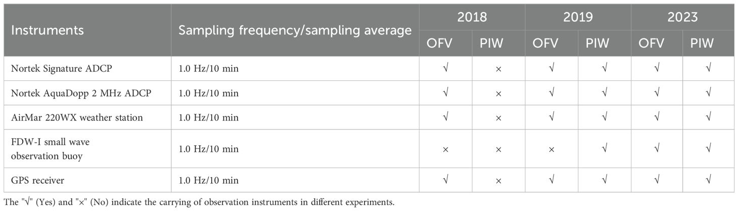
Table 1. Instruments utilized in the experiments.

Figure 1

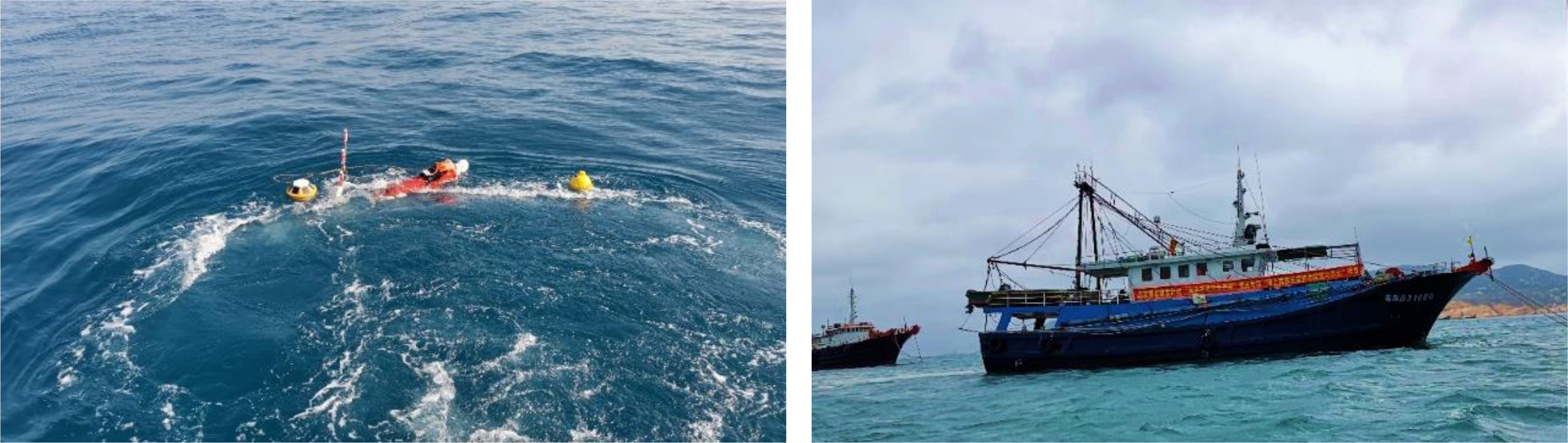
Figure 1. Horizontal PIW (left) and a typical Chinese OFV (right).

Figure 2

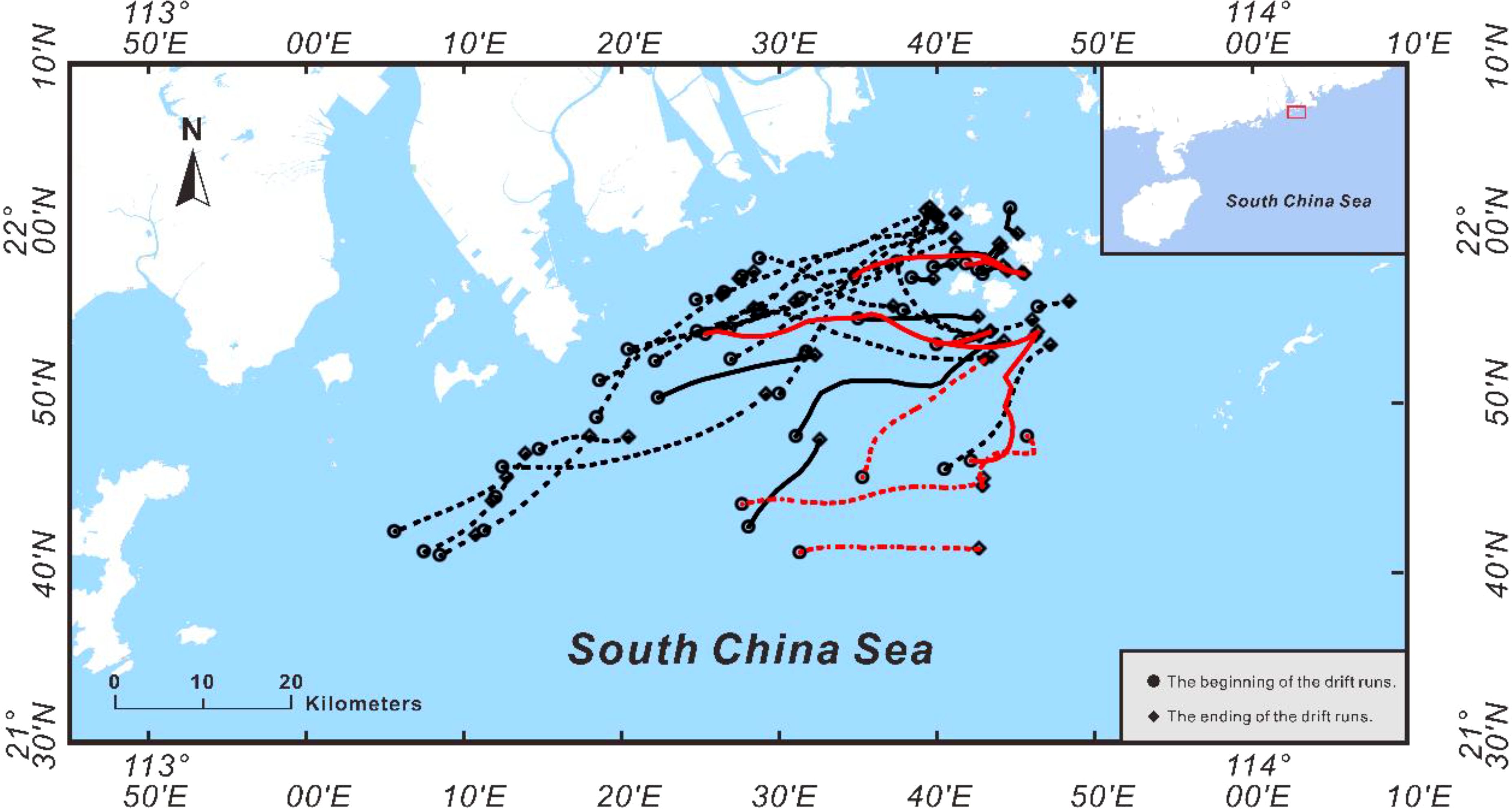
Figure 2. Drift trajectories and experimental area in the South China Sea. Drift trajectories of the OFV in 2018 (dash) and 2023 (solid) are plotted in black. Drift trajectories of the PIW in 2019 (solid) and 2023 (dash) are plotted in red.

2.2 Theoretical models and methods

2.2.1 Drift-prediction models for maritime SAR

The target-drift prediction method adopted in this study was the AP98 model combined with the Lagrange particle-tracking method adopted by most national SAR departments. According to the AP98 model, in the process of drifting at sea, the underwater part of the drifting target in distress is mainly affected by surface currents and waves, while the above-water part is mainly affected by wind. The sea target’s drift velocity is generally considered the superposition of the drift velocity caused by the above three factors (Allen, 2005; Breivik et al., 2011). Therefore, the drift velocity of a drifting target $\overrightarrow{V}$ at sea can be approximately expressed as follows:

$\begin{array}{ll}\overrightarrow{V}=\alpha {\overrightarrow{V}}_{sc}+\overrightarrow{L}+{\overrightarrow{V}}_{F-wave}& (1)\end{array}$

where ${\overrightarrow{V}}_{sc}$ represents the current velocity, and $\overrightarrow{L}$ and ${\overrightarrow{V}}_{F-wave}$ denote the WI and wave-induced drift velocities, respectively. The CI velocity is commonly assumed to be equivalent to the surface current velocity ${\overrightarrow{V}}_{sc}$, so $\alpha$ is generally approximated as 1. In previous target-drift prediction methods, the AP98 model was used to fit the remaining velocity (considered the WI drift velocity) after separating the CI drift velocity from the target-drift velocity, while the wave-drift velocity was ignored. Based on previous research, a target-drift prediction method considering wave-induced drift based on stepwise parameter calibration is proposed. First, current velocity is used to fit the target-drift velocity, and the CI drift coefficient $\alpha$ and residual ${ϵ}_c$ are obtained. Furthermore, wind speed is used to fit the components of residual ${ϵ}_c$ in the downwind and crosswind direction, and then the AP98 model coefficients and fitting residual ${ϵ}_L$ are obtained. Since wind and current are the main contributors to the target-drift velocity, the remaining fitting residual ${ϵ}_L$ can be considered to mainly include the wave-induced drift velocity’s influence. Figure 3 shows the parameters’ stepwise calibration’s schematic diagram.

Figure 3

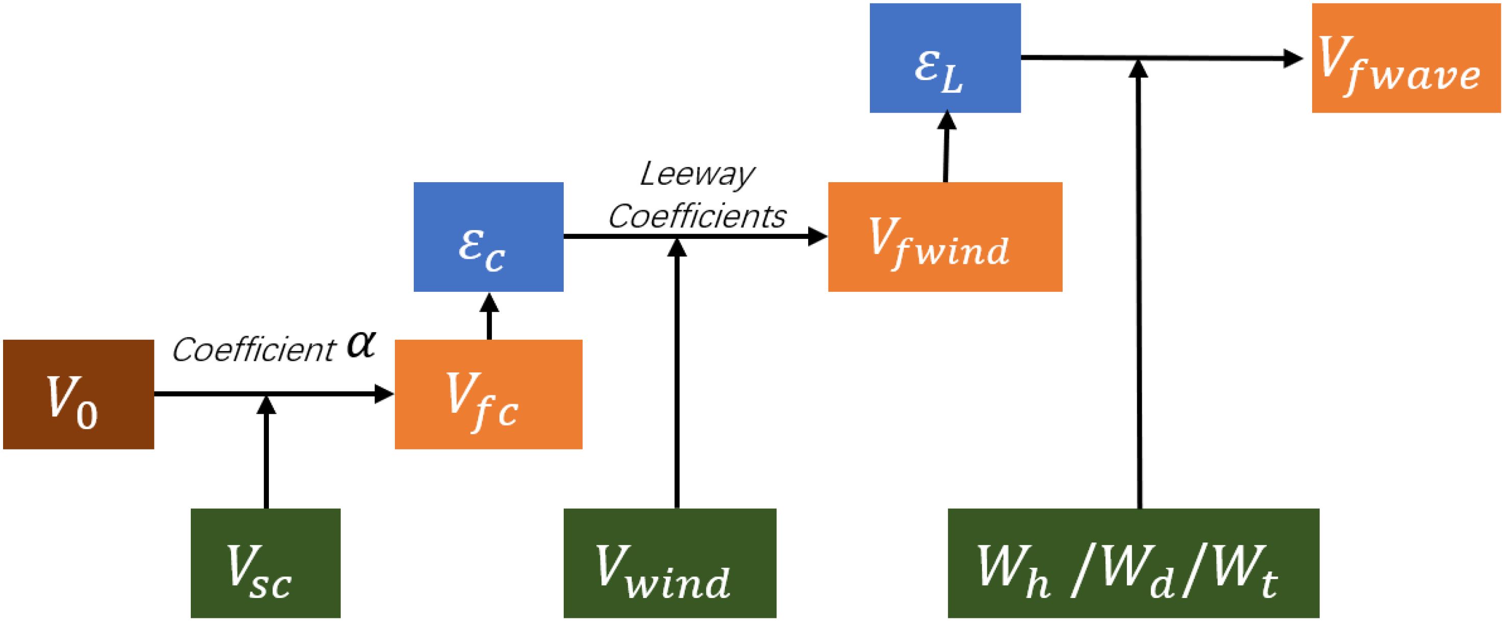
Figure 3. The stepwise parameter calibration.

Note that this stepwise parameter calibration method actually assumes that the fitting residual (or unexplained drift) after removing the WI and CI drift velocity is the contribution of wave-induced drift. This method is based on the assumption that wave-induced drift is less influential than current and wind. This is consistent with the idea of extracting WI drift velocity in previous studies, which essentially interprets WI drift velocity as the fitting residual after removing flow-induced drift.

The AP98 model (Allen and Plourde, 1999; Breivik et al., 2011) deconstructed the WI drift velocity into two components, DWL and CWL (Figure 4). The approximate linear relationship between the wind speed and these two components of the drifting object is as follows:

Figure 4

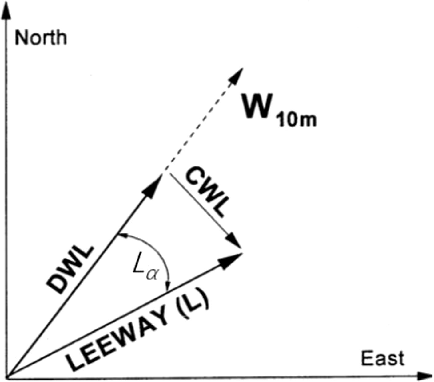
Figure 4. The leeway L consists of a DWL and aCWL.

$\begin{array}{ll}\{\begin{array}{ll}{L}_d=a_d{W}_{10m}+b_d+{ϵ}_d& \hspace{1em}(DWL)\\ L_{c+}=a_{c+}{W}_{10m}+b_{c+}+{ϵ}_{c+}& \hspace{1em}(+CWL)\\ L_{c-}=a_{c-}{W}_{10m}+b_{c-}+{ϵ}_{c-}& \hspace{1em}(-CWL)\end{array}& (2)\end{array}$

$L_d$, $L_{c+}$, and $L_{c-}$ represent the WI velocity vectors in the downwind, right crosswind, and left crosswind directions, respectively, which are related to the slope a, offset b, and the error term $ϵ$. $W_{10m}$ represents the wind speed at a height of 10 m. The error term $ϵ$ is calculated as $ϵ=norm*S_{y/x}$, where $norm$ is a random variable that follows the standard normal distribution, and $S_{y/x}$ represents the regression standard deviation.

2.2.2 Wave-induced drift simulation

After separating the effects of current and wind from the drift velocity of the target using the AP98 model, we can assume that the remaining fitting residuals ${ϵ}_L$ mainly include the effects of wave-induced drift velocity. After obtaining the wave-induced drift components, we use the numerical method based on FAM and the ML method to fit the wave-induced drift respectively.

2.2.2.1 Force analysis method

According to Tanizawa et al (2002), the mechanism of wave drift speed varies with wavelength. In short wave range, wave drift force due to wave scattering pushes the floating target. Therefore, drift speed is decided by the equilibrium of wave drift force F_W and fluid drag force F_D and it is proportional to the wave slope. Wave drift speed is obtained from the balance between F_W and F_D as follows:

$\begin{array}{ll}\frac{V}{\sqrt{D_{R}g}}=\frac{1}{2}\sqrt{\frac{{\lambda }^2{C}_W}{A{C}_D}}\frac{H_w}{\lambda }& (3)\end{array}$

where A is projection area of the buoy below the free surface, C_D is drag coefficient of the target, C_W is nondimensional wave drift force and D_R is the representative target scale. The values of C_D and C_W can be obtained from experiment, database or computation. In this paper, we call the coefficient a as the linear coefficient of wave drift speed.

$\begin{array}{ll}a=\frac{1}{2}\sqrt{\frac{{\lambda }^2{C}_W}{A{C}_D}}& (4)\end{array}$

In long wave range, on the other hand, wave drift force hardly acts on the floating target, because wave almost transmits the floating target. Therefore, the drift speed is decided by the wave-current speed and it is proportional to the square of the wave slope. Assuming that the drift speed of the target can be approximated by the average wave current speed on the projection area of the body, it is given by

$\begin{array}{ll}\frac{V}{\sqrt{D_{R}g}}=b{\left(\frac{H_w}{\lambda }\right)}^2=b{\sigma }^2& (5)\end{array}$

$\begin{array}{ll}b=\frac{{\pi }^2}{A\sqrt{k{D}_R}}{\displaystyle {\int }_A{e}^{2kz}ds}& (6)\end{array}$

where δ is wave slope Hw/λ, and b is the quadratic coefficient of wave drift speed.

Considering the results in the previous sections, we expected that wave drift speed in the entire wave range is approximated by the sum of the speed in the short wave range and that in the long wave range.

$\begin{array}{ll}\frac{V}{\sqrt{D_{R}g}}=a\sigma +b{\sigma }^2& (7)\end{array}$

The values of a and b are mainly related to the drag coefficient of the target, projection area of the buoy below the free surface, etc., which can be obtained from experiment, database or computation. However, under the experimental conditions in this work, since the wave-induced drift velocity has been obtained, we use the binomial fitting method to optimize the two values of a and b.

2.2.2.2 ML methods

Machine learning has been widely used in the field of modeling, including maritime SAR (Gao et al., 2023; Cao et al., 2024). In past studies, many scholars have explored wave drift’s influence with different analysis methods and different models. However, all models agree that wave-induced drift’s main influencing factors include wave height, wave direction, wave period, and factors related to the target size (e.g., surface and underwater area). Therefore, in addition to the factors related to the target, parameters including wave height, wave direction, and wave period were used as inputs to the wave-induced drift model, and three ML methods including LSTM, RF, and BP neural network were used to study wave-induced drift.

The LSTM neural network, a distinct architectural variant of recurrent neural networks (RNNs) (Hochreiter and Schmidhuber, 1997; Yu et al., 2019), has unique capabilities in processing sequential data. Figure 5 shows a schematic illustration of the LSTM structure (Yu et al., 2019). The LSTM model’s main steps are as follows: Step 1) The forgetting gate determines the information discarded from the cell state, using the sigmoid function to map the information values to the interval [0,1], where 0 indicates complete forgetting and 1 indicates complete retention; Step 2) the input gate determines which information to retain in the input information, and then the tanh activation function generates new candidate information, which is stored in the cell state; Step 3) the cell state is updated by forgetting a portion of the information via the forgetting gate and incorporating the candidate information through the input gate, resulting in a new cell state; Step 4) The information is entered into the updated cell state, and the characteristics of the output cell are determined by running a sigmoid function. The cell state value is transformed into the range of [−1,1] through the application of the tanh activation function, subsequently multiplied by the judgment condition derived from the sigmoid function, ultimately resulting in pertinent information’s output.

Figure 5

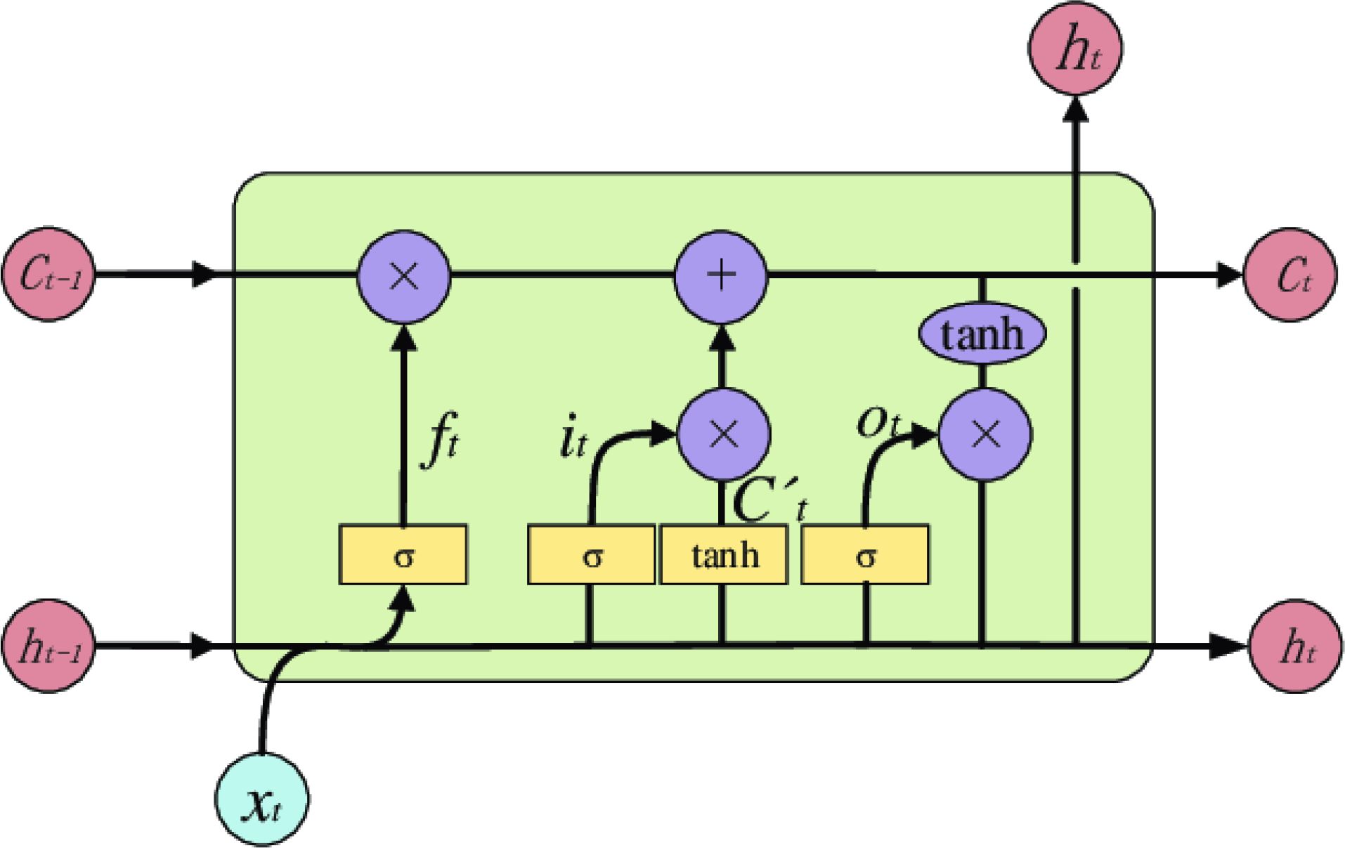
Figure 5. The LSTM’s schematic illustration.

The RF model, a variant of the parallel ensemble model known as Bagging, was introduced by Breiman, 2001. The RF model comprises multiple decision trees constructed by randomly selecting attributes. For regression tasks, predictions are made by averaging the outputs of these trees. The main steps for wave-induced drift prediction are as follows: Step 1) Input a training sample set comprising N combinations of forecast factors and predictor variables, with a total sample size of K; Step 2) draw m subsets of training samples, each with a sample size of K, from the overall training set using simple random sampling; Step 3) construct m decision trees using the m subsets of training samples. The node attributes of these trees are determined by randomly selecting n out of N indicators, following the random subspace theory; Step 4) based on the decision tree algorithm, each tree produces a single prediction. The final predicted value is then obtained by averaging the predictions from all m trees.

The BP neural network (Ding et al., 2011), also known as the feed-forward neural network, operates based on the fundamental principle of the BP algorithm, which distinguishes between forward- and backward-propagation phases during model execution. During the forward-propagation phase, input data traverse through the input layer and subsequent hidden layers and finally reach the output layer. Conversely, in the backward-propagation phase, the incorrect output (represented in a specific form) is propagated back from the output layer, traversing through each hidden layer in reverse order until it reaches the input layer. The output layer’s primary function is to transmit the error information along the transmission route, first to the hidden layers and then back to the input layer, ultimately facilitating the adjustment of the weights of individual network units. Figure 6 shows the BP neural network’s structure (Ding et al., 2011).

Figure 6

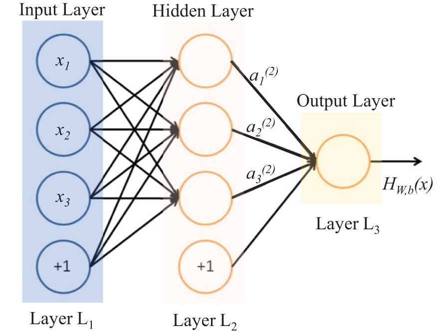
Figure 6. The BP neural network’s structure.

3 Model calibration

Three experiments in total were conducted on the OFV and the PIW, of which wind and current observations were fully recorded in 2018, 2019, and 2023, while wave observations were only of high quality in 2023. Therefore, for an OFV, a total of 1,632 sample data points in 2018 and 2023 were used for parameter calibration to fit the WI drift and CI drift. For the PIW, a total of 622 sample data points in 2019 and 2023 were used for parameter calibration to fit the WI drift and CI drift. Based on the fitting coefficients of the wind and current drift models, combined with the observation data of 2023 (316 PIW samples, 432 OFV samples), the WI and CI drift velocities were separated from the target-drift velocities, and the wave-drift velocities were fitted.

3.1 Fitting of CI and WI drift velocities

First, the current velocities in the north–south and east–west directions were taken as the input, and the drift velocities in the north–south and east–west directions were taken as the output. The drift coefficient of the current $\alpha$ was calculated to be 0.96 by the least-square method. The residuals (residual velocities) ${ϵ}_1$ obtained by fitting target-drift velocities with current velocities were used as the output of WI drift velocity fitting, and the residual velocities were deconstructed into downwind and crosswind directions. Then, taking wind speed as input, we used the AP98 model to fit the downwind, crosswind, and total velocities of residuals.

Figures 7, 8 show the residuals ${ϵ}_1$ fitted for the OFV and the PIW drift velocity, respectively, and their corresponding wind velocities rose plots. From these results, it can be considered that the residual velocities, after removing the CI drift velocities, were mainly affected by wind and waves. It also can be found from Figures 6, 7 that the directions of residual velocities were highly consistent with the wind direction, and that they were basically distributed on both sides of the wind direction.

Figure 7

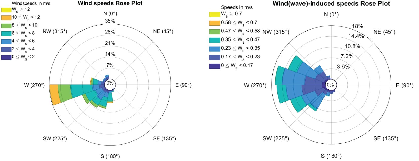
Figure 7. The rose diagrams of wind velocities (left) and residuals ${ϵ}_1$ (wind and wave-induced drift velocities) (right) for OFV.

Figure 8

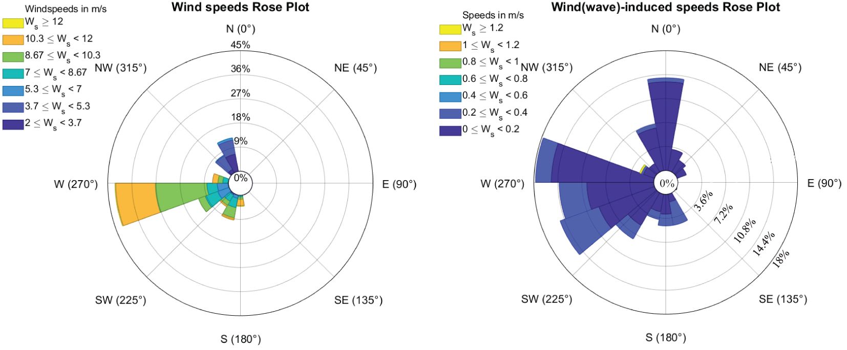
Figure 8. The rose diagrams of wind velocities (left) and residuals ${ϵ}_1$ (wind and wave-induced drift velocities) (right) for the PIW.

Figures 9, 10 and Table 2 show the parameter-calibration results of the AP98 model for the OFV and the PIW using these residuals ${ϵ}_1$. Note that for crosswind WI drift, 72% of an OFV’s crosswind samples fell in the right side of the downwind direction (+CWL), while 55% of PIWs crosswind samples fell in the right side of the downwind direction (+CWL).

Figure 9

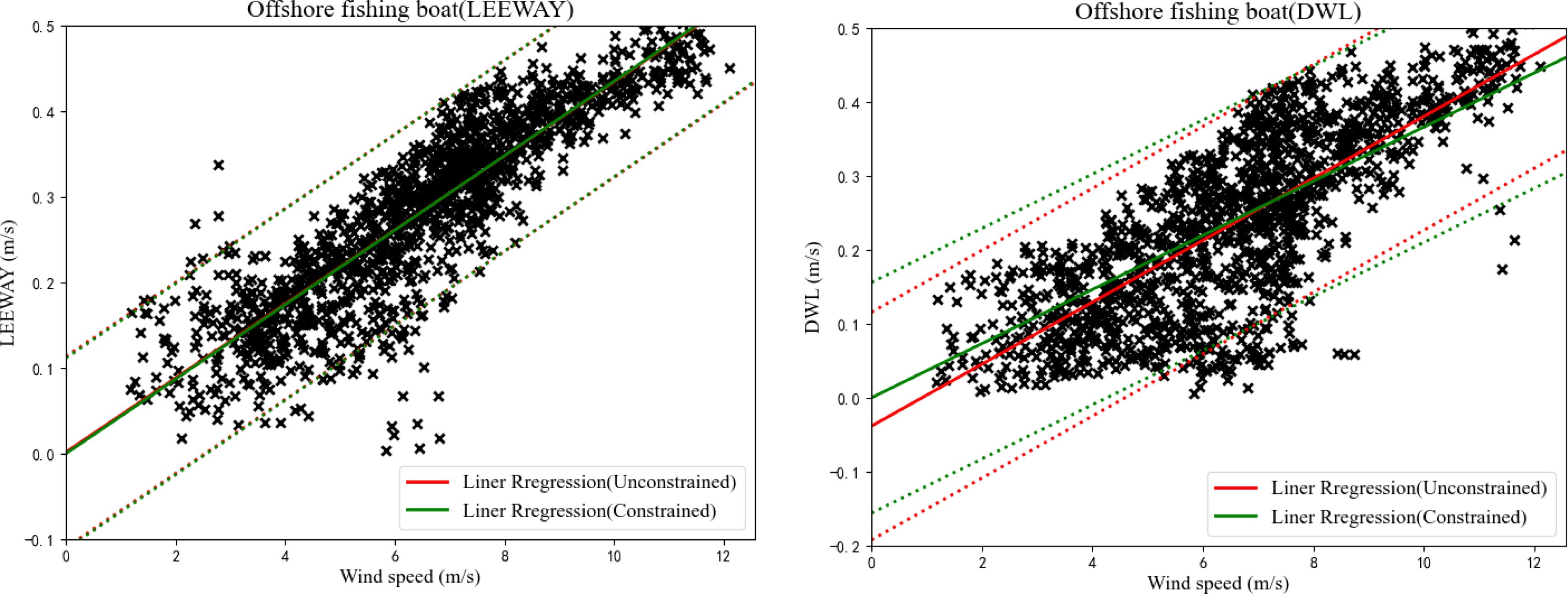
Figure 9. Leeway speed (left) and DWL (right) versus wind speed adjusted to a 10-m height for the OFV. Unconstrained linear regression (solid) and 95% of the confidence levels (dash) are plotted in red, while constrained linear regression is plotted in green.

Figure 10

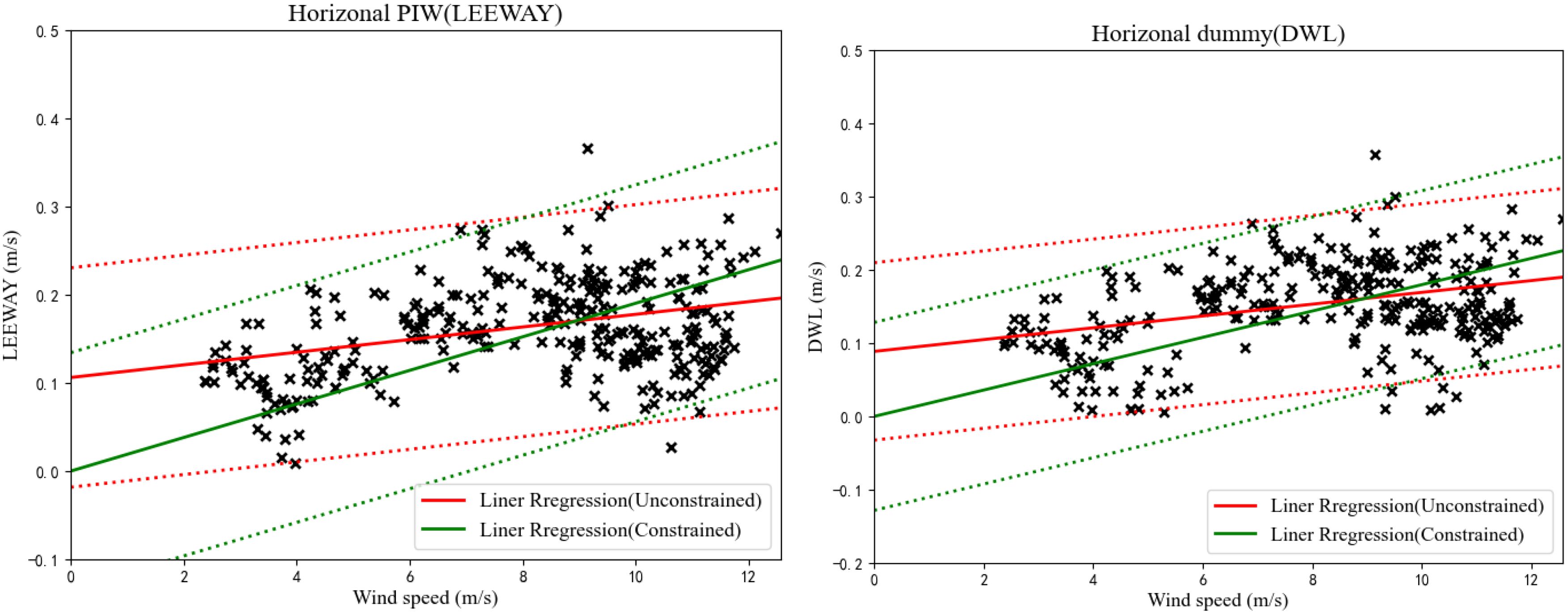
Figure 10. Leeway speed (left) and DWL (right) versus wind speed adjusted to a 10-m height for the PIW. Unconstrained linear regression (solid) and 95% of the confidence levels (dash) are plotted in red, while constrained linear regression is plotted in green.

Table 2

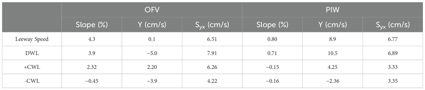
Table 2. Linear regression of leeway parameters.

3.2 Fitting of wave-induced drift velocities

The TensorFlow deep-learning framework was utilized in this study, and the pre-processed data were subsequently imported into each of the three neural-network models through Python programming tools. To ensure a balanced approach to model development and validation, we allocated 80% of the data for training purposes and the remaining 20% for testing.

The FDW-I wave buoy model was employed. The observed wave-related parameters encompassed the mean wave period, mean wave height, main wave direction, significant wave height, and significant wave period. The mean wave height (period) is the average of all observed wave heights (periods) in an observation period, while the significant wave height (period) refers to the average of the first n/3 waves in a wave train, which is arranged from the largest to the smallest wave height in an observation period. During the experiments, the significant wave height ranged from 0.29 m to 1.31 m, the mean wave height ranged from 0.21 m to 1.13 m, the significant wave period ranged from 2.4 s to 5.0 s, the mean wave period ranged from 2.6 s to 5.1 s.

3.2.1 Force analysis method

The scales of PIW and OFV were set to 26.3 m and 1.93 m respectively. The wave-induced velocity V was decomposed into east-west and north-south components and then brought into the following quadratic polynomials for fitting.

$\begin{array}{ll}{B}_m=\frac{V}{\sqrt{D_{R}g}}=a\sigma +b{\sigma }^2& (8)\end{array}$

Where, $\sigma =\frac{H_w}{\lambda }$. $H_w$ is the significant wave height, and $\lambda =\frac{T^{2}g}{2\pi }$. The cost function can be constructed as:

$\begin{array}{ll}F(a,b,\sigma )={\displaystyle \sum _{m=1}^M{[(a{\sigma }_m+b{\sigma }_m{}^2)-B_m]}^2}& (9)\end{array}$

Taking the partial derivative of a and b to zero. For PIW, the optimal solution of a and b are 1.52 and 3.69, respectively. For OFV, the optimal solution of a and b are 2.18 and 2.29, respectively.

3.2.2 ML methods

To study the difference in prediction effect caused by different wave-parameter settings (e.g., the angle between wave direction and wind and current), we set up different schemes (S1–S8, Table 3) to establish the LSTM, BP neural network, and RF models.

Table 3

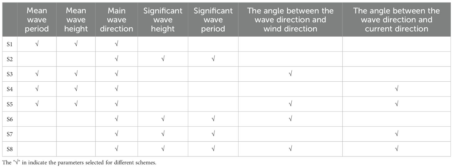
Table 3. Eight schemes for the fitting of wave-induced drift velocities.

The LSTM model adopts parameter settings outlined by Zhao et al., 2017, and the neural-network model’s hyper-parameters were determined through a trial-and-error approach. After comprehensive consideration of the model’s prediction results and calculation time, the number of hidden layers was set to 2, the initial learning rate was set to 0.005, and the loss rate was set to 0.01. The model was trained and optimized using the adaptive moment estimation (Adam) algorithm, the root mean square error (RMSE) was employed as the objective function for the optimization procedure, the maximum number of iterations was set to 250, and the number of hidden-layer neural units was set to 128.

The setting of the BP neural network model’s input parameters depends on the selected parameter scheme. When the input parameters are the average wave period, mean wave height, and main wave direction, the input layer data parameter n_input is 3. Since the purpose of this experiment was to fit the velocities of wave-induced drift in the north–south and east–west directions, the output layer n_output was 2. The number of hidden layer neurons here was set to 15, while the learning rate was set to 0.0001.

In constructing the RF model, the number of decision trees was determined to be 100 through the trial-and-error method. In addition, the minimum number of leaves was set to 5, adhering to the parameter-setting methodology outlined by Schoppa et al. (2020).

The statistical metrics commonly employed in this field—namely, the RMSE and scaled Nash efficiency coefficient (NSE)—were chosen as the primary evaluation metrics to evaluate the performance of the aforementioned three ML modeling schemes.

$\begin{array}{ll}NSE=1-\frac{{\displaystyle {\sum }_{i=1}^N{(x(t)-\widehat{x}(t))}^2}}{{\displaystyle {\sum }_{i=1}^N{(x(t)-\overline{x}(t))}^2}}& (10)\end{array}$

$\begin{array}{ll}RMSE=\sqrt{\frac{{\displaystyle {\sum }_{i=1}^N{(x(t)-\widehat{x}(t))}^2}}{N}}& (11)\end{array}$

where $x(t)$ and $\widehat{x}(t)$ represent the actual and fitted wave-induced drift velocities, respectively. $\overline{x}$ is the mean value of the actual wave-induced drift velocity. N is the length of the samples. The closer the NSE value is to 1, the better the simulation effect. The smaller the RMSE value, the higher the fitting accuracy.

4 Results and discussions

4.1 ML fitting results of wave-induced drift velocities

In this study, we employed three distinct ML methodologies to model the wave-induced drift velocities. Note that the fitting of wave-induced drift velocities was divided into two components: north–south velocities and east–west velocities. However, we calculated RMSE and NSE by combining the north–south and east–west samples to ensure the overall wave-induced drift velocities’ best fitting.

4.1.1 LSTM neural-network model

The outcomes of the model evaluation, utilizing eight distinct schemes within an LSTM neural-network framework for two different targets, the OFV and the PIW, are presented in Figure 11 and Table 4, respectively. For an OFV, the model accuracy was the highest when scheme S6 was adopted, for which the RMSE and the NSE were 0.041 and 0.47, respectively. The remaining values in the table are the proportion of the increase in RMSE and NSE values relative to the optimal scheme S6. Similarly, for the PIW, the model accuracy was the highest when scheme S8 was adopted, and the RMSE and the NSE were 0.055 and 0.34, respectively. The remaining values in the table are the proportion of the increase in RMSE and NSE values relative to the optimal scheme, S8.

Figure 11

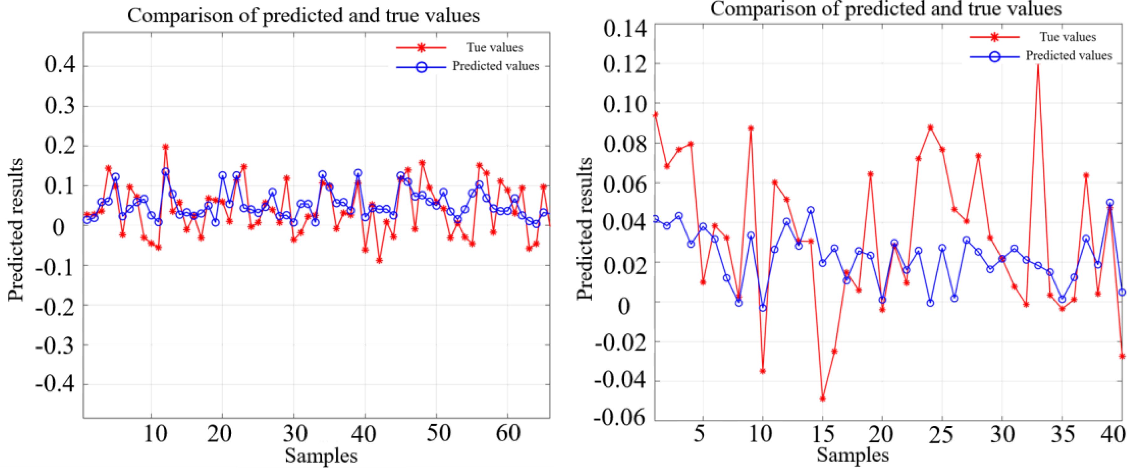
Figure 11. The comparison between the true value and the fitting value of the wave-induced drift velocity of the OFV (left) and the PIW (right) using the optimal scheme based on the LSTM.

Table 4

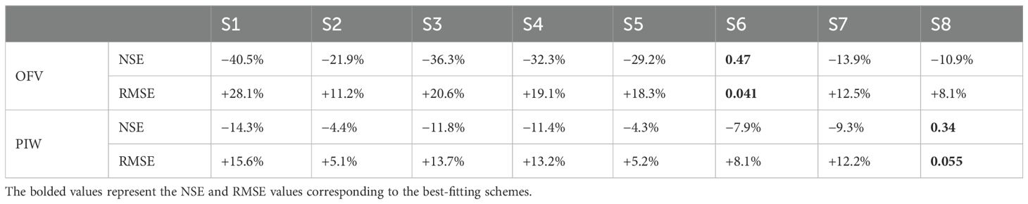
Table 4. Evaluation results of eight scheme models based on the LSTM.

4.1.2 Training results of BP neural network

The evaluation results of the BP neural-network model, employing eight schemes for the OFV and the PIW, are shown in Figure 12 and Table 5. For an OFV, the model accuracy was the highest when scheme S6 was adopted, and the RMSE and the NSE were 0.05 and 0.39, respectively. The remaining values in the table are the proportion of the increase in RMSE and NSE values relative to the optimal scheme S6. Similarly, for the PIW, the model accuracy was the highest when scheme S2 was adopted, and RMSE and the NSE were 0.059 and 0.32, respectively. The remaining values in the table represent the proportion of the increase in RMSE and NSE values relative to the optimal scheme S2.

Figure 12

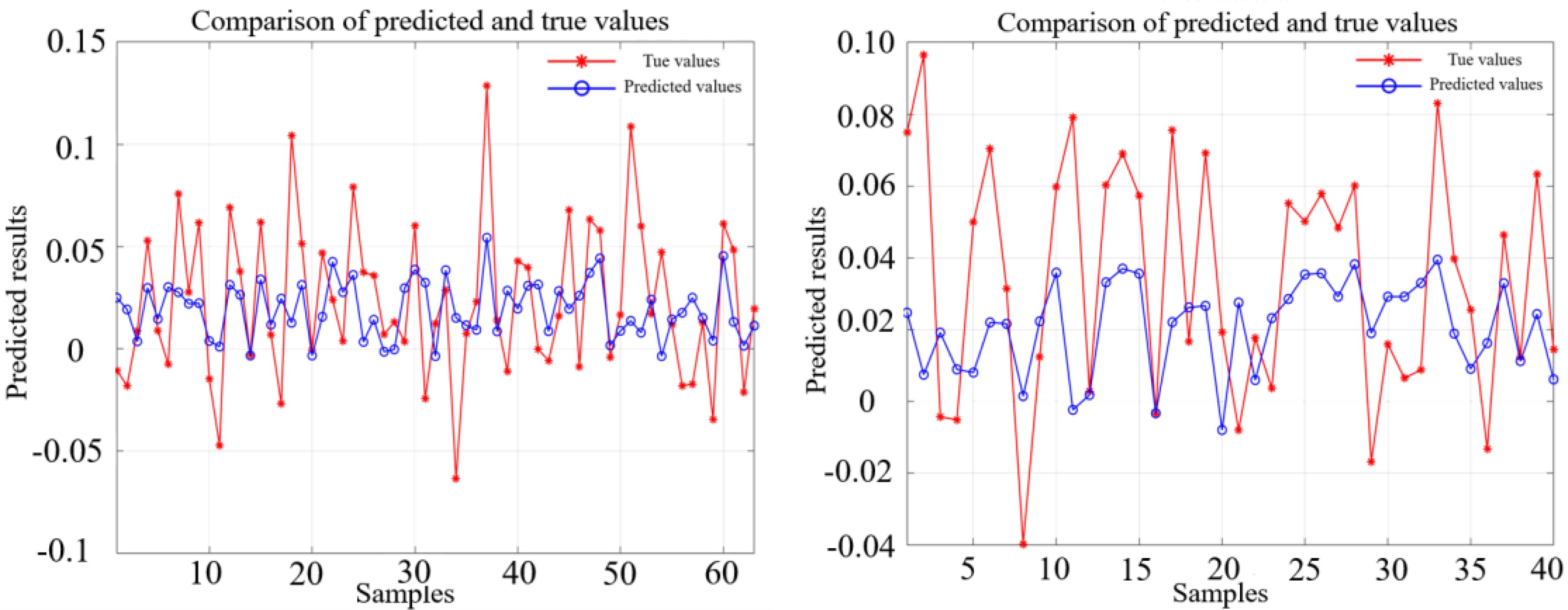
Figure 12. The comparison between the true value and the fitting value of the wave-induced drift velocity of the OFV (left) and the PIW (right) using the optimal scheme based on the BP neural network.

Table 5

Table 5. Evaluation results of eight scheme models based on the BP neural network. .

4.1.3 Training results of the RF model

The evaluation results of the RF model, employing eight schemes for the OFV and the PIW, are presented in Figure 13 and Table 6. For an OFV, the model accuracy was the highest when scheme S8 was adopted, and the RMSE and the NSE were 0.048 and 0.42, respectively. The remaining values in the table are the proportion of the increase in RMSE and NSE values relative to the optimal scheme S6. Similarly, for the PIW, the model accuracy was the highest when scheme S2 was adopted, and the RMSE and the NSE were 0.053 and 0.36, respectively. The remaining values in the table are the proportion of the increase in RMSE and NSE values relative to the optimal scheme S2.

Figure 13

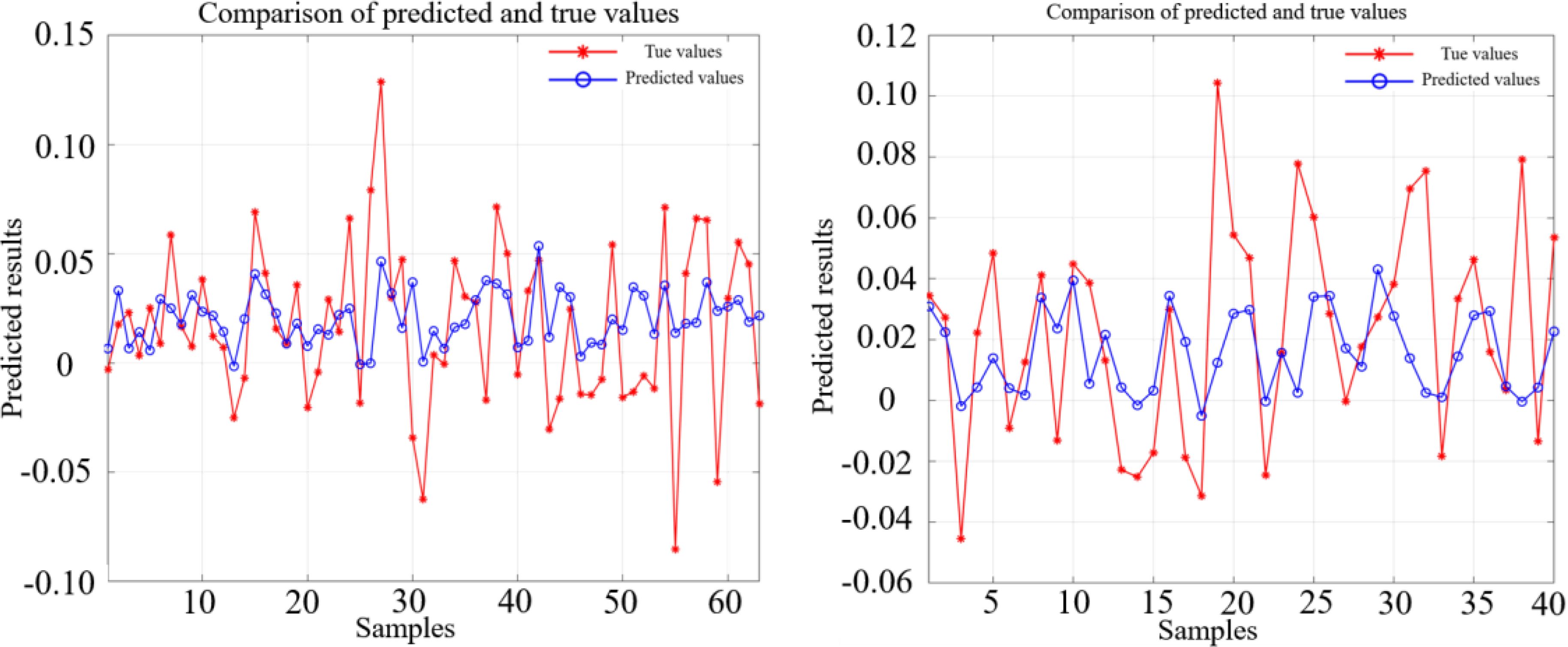
Figure 13. The comparison between the true value and the fitting value of the wave-induced drift velocity of the OFV (left) and the PIW (right) using the optimal scheme based on the RF model.

Table 6

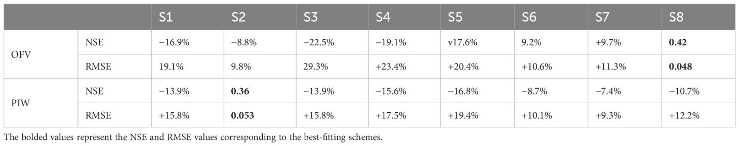
Table 6. Evaluation results of eight scheme models based on the RF model.

By analyzing the evaluation results of the above three ML models trained with eight different parameter setting schemes, we could make the following preliminary observations:

(1) According to the evaluation results of three ML methods, for an OFV, the LSTM neural network with optimal scheme S6 had the best-fitting effect on wave-induced drift velocities, followed by the RF model, and the BP neural network. For the PIW, the RF model using the optimal scheme S2 had the best-fitting effect on wave-induced drift velocities, followed by the LSTM, and the BP neural network;

(2) From the evaluation results of eight different parameter schemes, no matter which ML model was used, the schemes using the significant wave height and significant wave period (S2, S6, S7, S8) were generally better than the schemes using the average wave height and average wave period (S1, S3, S4, S5);

(3) From the comparison of model evaluation results for two different target types, the fitting result of wave-induced drift for an OFV was significantly better than that of the PIW. This indicates that wave-induced drift of an OFV is more strongly correlated with waves to a certain extent, which is also consistent with some previous studies’ conclusions on the relationship between wave-induced drift and target size. In addition, factoring in the wave direction, current, and especially the wind, could also improve the model’s accuracy to some extent, although its impact was not very significant compared with all results;

(4) By analyzing the contribution of wind, wave, and current to the target-drift velocity in all samples, we found that for an OFV, the average drift velocity caused by current was about 0.429 m/s, the average drift velocity caused by wind was about 0.227 m/s, and the average drift velocity caused by waves was about 0.075 m/s. Moreover, for the PIW, the average drift velocity caused by current was about 0.452 m/s, the average drift velocity caused by wind was about 0.238 m/s, and the average drift velocity caused by waves was about 0.041 m/s. Therefore, for both target types, current was the main factor leading to target-drift motion, the wind was the second most influential factor, and the wave influence was relatively small, consistent with our assumption that the parameter stepwise calibration method was adopted.

4.2 Comparison of trajectory prediction

To further validate wave-induced drift’s influence on the drifting behavior of sea targets, the previously established wave-induced drift model’s optimal schemes [PIW (RF, S2), an OFV (LSTM, S6)] and the FAM model were used to calculate and compare drift trajectory and ensemble trajectory predictions for the two targets.

The samples used to calculate drift trajectories and ensemble-trajectory predictions were independent of the samples used for ML training and evaluation. Among them, two cases of OFV samples were used for drift trajectory calculations, with continuous experimental observation durations of 13 and 9 h. There were also two cases of PIW samples used for drift trajectory calculations, with continuous experimental observation durations of 6 and 8 h.

The prediction of the trajectory was conducted utilizing the Lagrange particle tracking method (Drouin et al., 2019). The drift motion of the sea target can be expressed by the following formula:

$\begin{array}{ll}\overrightarrow{x}(t)-\overrightarrow{x_0}={\displaystyle {\int }_0^t\overrightarrow{V_o}(t^{\text{'}})}d{t}^{\text{'}}={\displaystyle {\int }_0^t\left[\alpha {\overrightarrow{V}}_{sc}(t^{\text{'}})+\overrightarrow{L(t^{\text{'}})}+{\overrightarrow{V}}_{F-wave}(t^{\text{'}})\right]}d{t}^{\text{'}}& (12)\end{array}$

$\overrightarrow{x_0}$ and $\overrightarrow{x}(t)$ denote the initial and current position of the target, respectively. In instances where the wave-induced drift’s influence was neglected, there was ${\overrightarrow{V}}_{F-wave}=0$, $L_d=a_d{V}_{wind}+b_d+{ϵ}_d$. Here, ${ϵ}_d=S_{y/x}·norm$, where $norm$ is a random number that followed normal distribution N(0,1), and $S_{y/x}$ represents the standard deviation of WI drift velocities fitted by the AP98 model.

When the effect of wave-induced drift was considered, there was $L_d=a_d{V}_{wind}+b_d$, ${\overrightarrow{V}}_{F-wave}={\overrightarrow{V^{\prime }}}_{F-wave}+{ϵ}_w$, ${ϵ}_d=S_{y/x}·norm$, where $S_{y/x}$ represents the standard deviation of the wave-induced drift velocities fitted by the corresponding ML model.

Figures 14, 15 show the target drift trajectories obtained by the AP98 model, the AP98 model combined with the ML methods, and the AP98 model combined with FAM to simulate wave-induced drift, respectively. For the OFV cases, the simulated trajectories utilizing the LSTM to calculate wave-induced drift exhibited closer proximity to the observed real trajectories. Conversely, for the PIW cases, the trajectories simulated by the FAM or RF model did not approximate the real values as closely as those simulated trajectories directly using the AP98 model. Given that random disturbance terms were used in both trajectory simulation methods, the results of a single trajectory simulation were not completely representative. Therefore, the method of ensemble-trajectory prediction was adopted to calculate the two cases of samples for the OFV and the PIW.

Figure 14

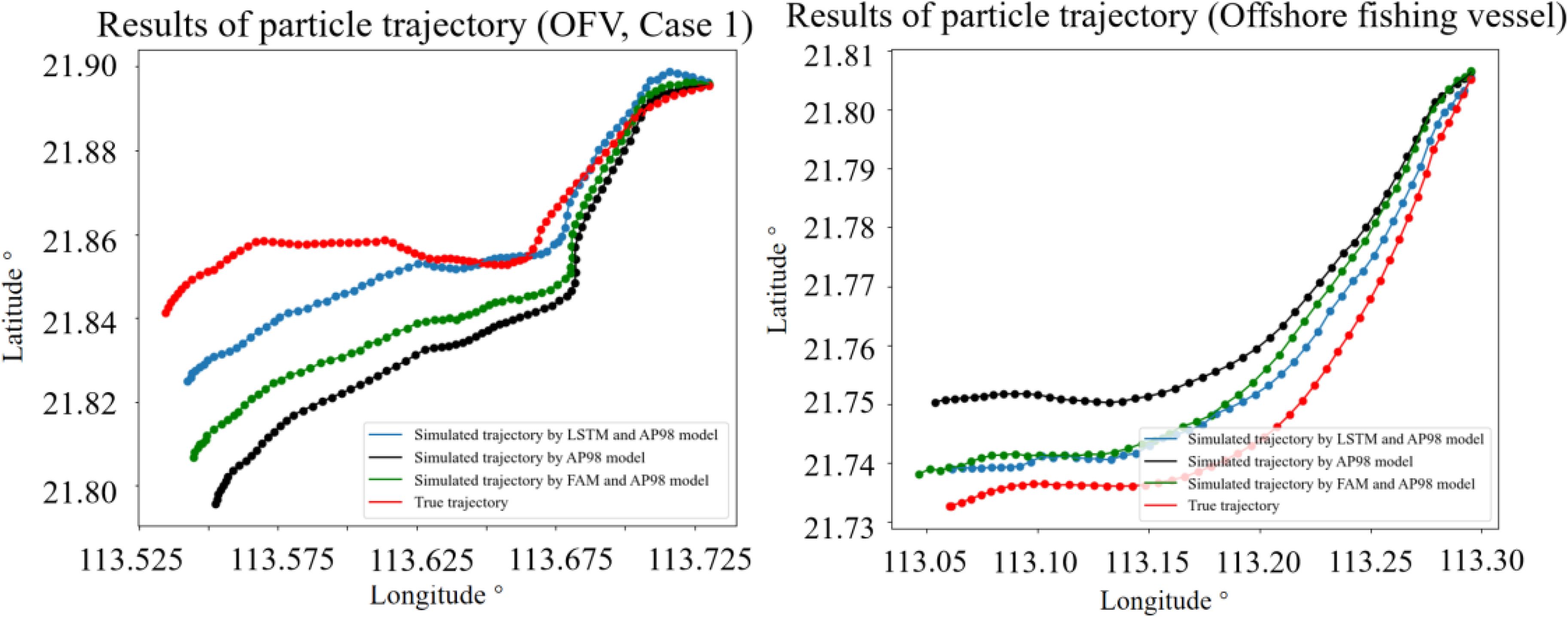
Figure 14. The results of particle trajectory obtained by 3 simulation schemes for the OFV.

Figure 15

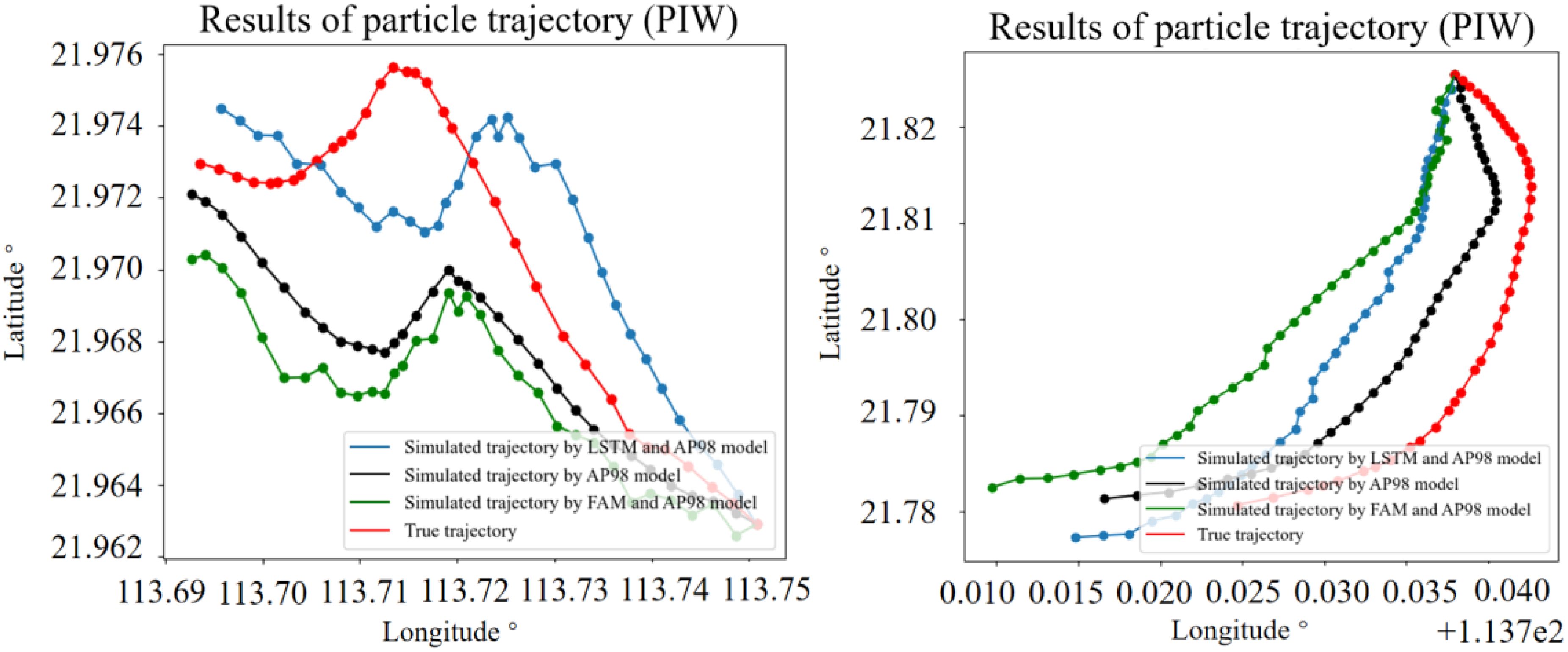
Figure 15. The results of particle trajectory obtained by 3 simulation schemes for the PIW.

4.3 Comparison of ensemble-trajectory predictions

The ensemble-trajectory prediction approach generated 1,000 particles for each case, and the trajectory prediction of each particle was calculated using Eq. (5). The difference was that for WI drift velocities, the random disturbance term was the fitting standard deviation of the AP98 model; for the wave-induced drift, the random disturbance term was the fitting standard deviation of the LSTM, RF and FAM model.

The range predicted by the model was determined by the horizontal position distribution of the simulated particles at different times. In this work, a closed curve containing 98% particle positions was calculated using the kernel density estimate method (Abascal et al., 2009a; Martinez, 2002) and the region contained in this curve was the predicted search range with a confidence interval of 98%. For a sample of size n, where each observation was a d-dimensional vector, X_i, i = 1,…,n, the kernel density estimate was defined as (Martinez, 2002):

$\begin{array}{ll}{\widehat{f}}_{Ker}(X)=\frac{1}{n{h}_1\dots h_d}{\displaystyle \sum _{i=1}^n\left\{{\displaystyle \sum _{j=1}^d\kappa \left(\frac{x_j-X_{ij}}{h_j}\right)}\right\}}& (13)\end{array}$

where X_ij is the jth component of the ith observation, $\kappa$ is the kernel function, and $h$ is the smoothing parameter or window width. The parameter h was defined as

$\begin{array}{ll}{h}_{jKer}={\left(\frac{4}{n(d+2)}\right)}^{\frac{1}{d+4}}{\sigma }_j;j=1,\dots ,d& (14)\end{array}$

where ${\sigma }_j$ is the standard deviation of the jth component. The kernel equation for density estimation was considered a Gaussian function:

$\begin{array}{ll}\kappa (x)=\frac{1}{\sqrt{2}\pi }\exp (\frac{-x^2}{2})& (15)\end{array}$

The calculation results of different ensemble-trajectory prediction schemes for the two cases of OFV samples are shown in Figure 16. Similarly, the results of different ensemble-trajectory prediction schemes for the two cases of PIW samples are shown in Figure 17. The area indicated by the gray dashed line is the predicted search area every hour, while the bold green points on the real trajectory are the target positions given at each interval of 1 h as well. The statistical situation of whether the prediction area successfully covered the real trajectory of the target is shown in Table 7.

Figure 16

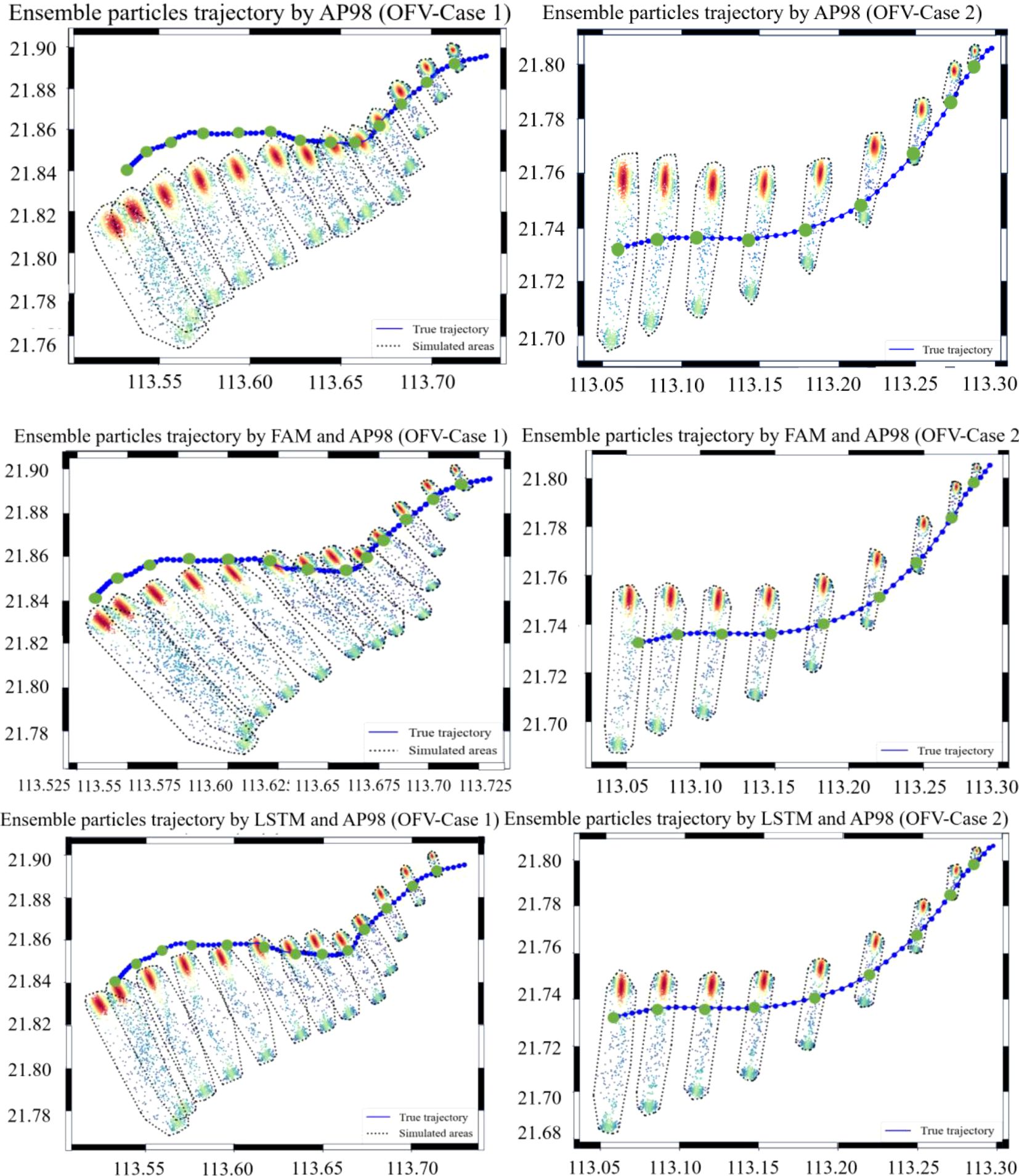
Figure 16. The ensemble-trajectory prediction results for two cases of an OFV obtained by 3 simulation schemes. The bold green points on the real trajectory are the target positions given at each interval of 1 h.

Figure 17

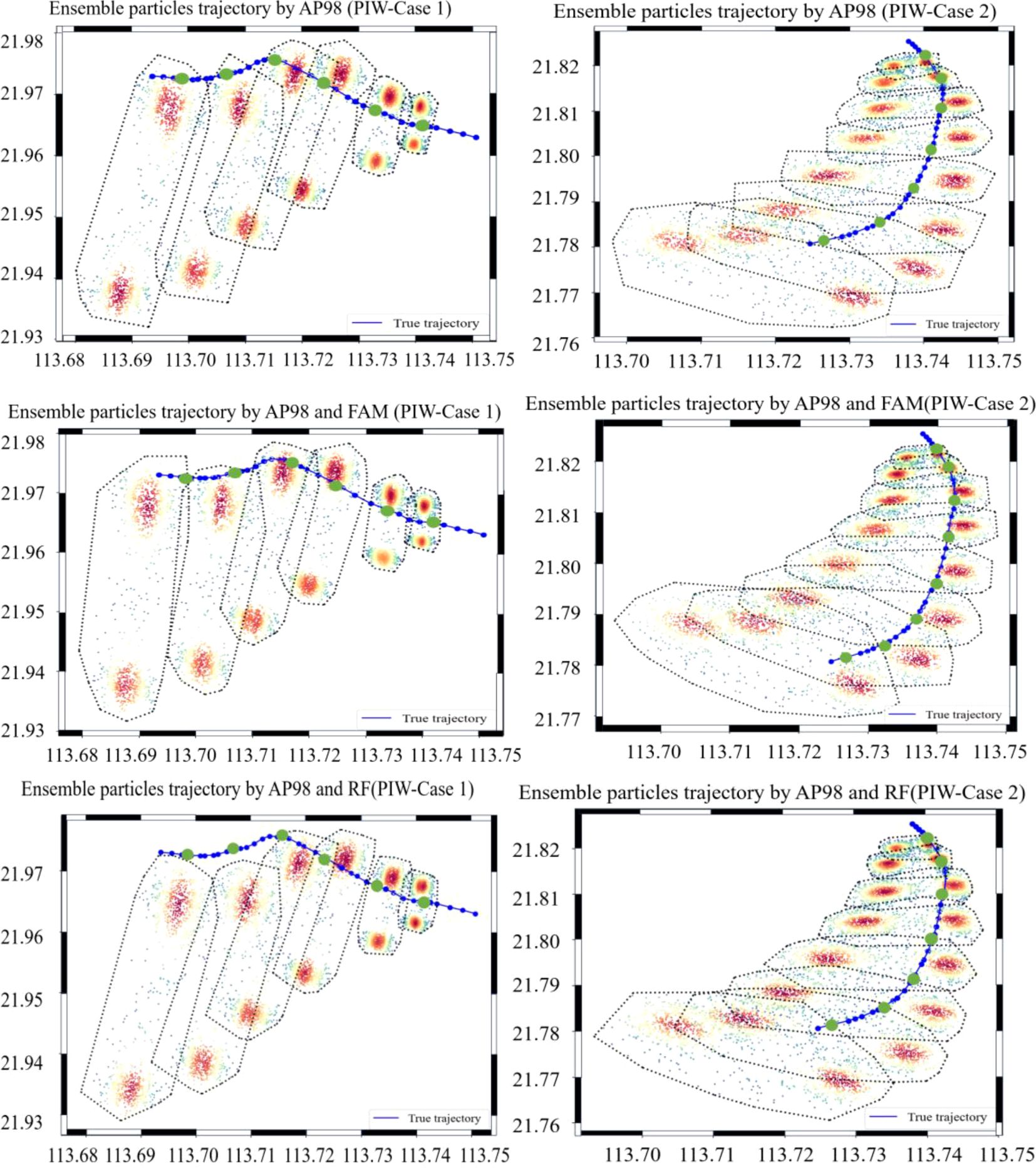
Figure 17. The ensemble-trajectory prediction results for two cases of PIWs obtained by 3 simulation schemes. The bold green points on the real trajectory are the target positions given at each interval of 1 h.

Table 7

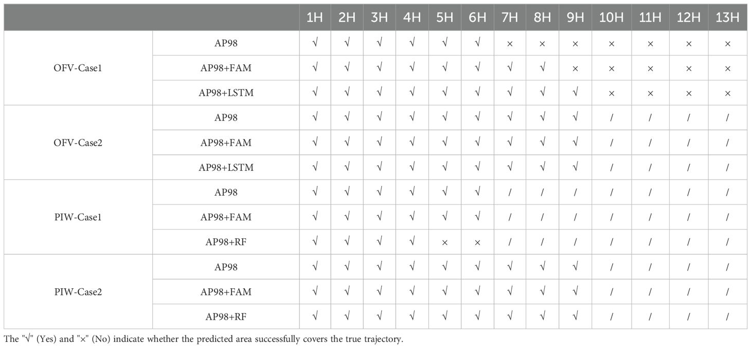
Table 7. The statistical situation of whether the prediction area successfully covers the real trajectory every hour.

The color of the points in the plot represents the probability of particle distribution density calculated from the kernel density estimate. It can be found from Figure 14 that in the prediction results of an OFV, particles were more concentrated on one side of the prediction range because the ensemble-trajectory prediction model took into account that for an OFV, the distribution probability of the crosswind component was much greater on the right side than on the left side. The average distance errors of the ensemble-trajectory prediction for the two target types are shown in Table 8. The average distance error was calculated every hour, and the value was equal to the average distance between the position of 1,000 particles simulated at the current time and the real target position.

Table 8

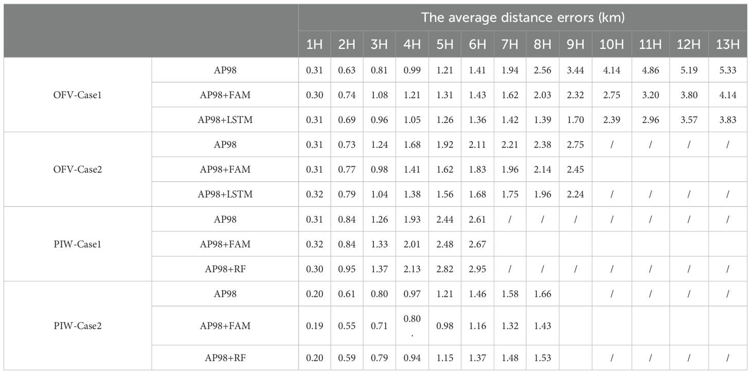
Table 8. The average distance errors of the ensemble-trajectory prediction for the OFV and the PIW.

It can be found from Table 8 and Figures 16, 17 that the average prediction errors of different schemes for target trajectory prediction were superimposed over time. In addition to the prediction results of the first 5 h in Case 1, the simulation results of the LSTM and FAM model for the two cases of OFV samples were superior to the AP98 model, and the longer the prediction time, the greater the difference in prediction accuracy between the two prediction schemes. When the simulation period was 13 h, the average distance error of the AP98 model for Case 1 reached 5.33 km, while the average distance error of AP98 combined with the LSTM model and FAM was 3.83 km and 4.14 km, respectively. When the simulation period was 9 h, the average distance error of the AP98 model for Case 2 reached 2.75 km, while the average distance error of AP98 combined with the LSTM model and FAM was 2.24 km and 2.45 km, respectively. In addition, it can be seen from Table 7 that the predicted range of the scheme using the LSTM or FAM combined with the AP98 model better covered the real trajectory. Thus, the simulation schemes considering wave-induced drift played a positive role in the OFV trajectory prediction. For the simulation of wave drift, the LSTM model was better than FAM in 2 cases.

In the comparison of the two cases for the PIW, the ensemble prediction trajectory simulated by two different schemes showed different results. In Case 1, the average distance error of the AP98 model, without considering wave-induced drift, was smaller than that of the AP98 combined RF model or FAM at every moment. The average prediction distance error of the AP98 model at the 6th hour was 2.61 km, while that of the AP98 combined RF model and FAM was 2.95 km and 2.67 km, respectively. However, the opposite result was observed in Case 2, where the AP98 model had an average distance error of 1.66 km at the 8th hour, while the AP98 combined with the RF model and FAM had an average distance prediction error of 1.53 km and 1.43 km. In addition, it can be seen from Table 7 that the predicted range of the scheme using RF or FAM combined with the AP98 model did not better cover the real trajectory. Therefore, it can be preliminarily found that the RF model considering wave-induced drift did not significantly improve the trajectory prediction accuracy for the PIW.

5 Conclusions and recommendations

A target-drift prediction method considering wave-induced drift based on stepwise parameter calibration was studied in this work. According to the analysis of the main contribution sources to the drift motion of the sea target, the CI drift and WI drift were separated from the target-drift motion based on the AP98 model. The residual velocity errors were derived from fitting the wave-induced drift velocities. Based on the field-observation experiments of two typical SAR targets, FAM and three kinds of ML methods combined with eight different parameter schemes were set up to fit the wave-induced drift of the OFV and the PIW. For an OFV, based on the LSTM model, the wave-induced drift fitting had the best effect when using the main wave direction, significant wave height, significant wave period, and the angle between wave and wind as model inputs. For the PIW, based on the RF model, the wave-induced drift fitting using the main wave direction, significant wave height, and significant wave period as model inputs produced the best effect. Finally, for the two target types, the two ML schemes with the best-fitting effect were selected to carry out trajectory simulation and ensemble-trajectory predictions for comparison.

In two sets of verification experiments for the OFV, the simulation results of LSTM and FAM models considering wave-induced drift were superior to the AP98 model for both OFV samples except the prediction results in the first 5 h of case 1. At the end of the trajectories in Case 1, the trajectory prediction errors obtained by best-fitting wave-induced drift based on the FAM and ML methods were reduced by 22.3% and 28.1%, respectively, compared with the trajectory prediction errors without considering wave-induced drift. For Case 2, the trajectory prediction errors obtained by best-fitting wave-induced drift based on the FAM and ML methods were reduced by 10.9% and 18.5%, respectively. From the experimental comparison results, when the OFV size was close to the wavelength, the ensemble-trajectory prediction results of the AP98 model combined with the LSTM model were significantly better than those only using the AP98 model, which indicates that considering wave-induced drift as part of the AP98 model can significantly improve the trajectory simulation accuracy for an OFV. Compared with the two cases of PIW prediction results, the accuracy of the RF model combined with the AP98 model or FAM considering wave-induced drift was not significantly improved. This result indicates that wave-drift effect on small targets including a PIW is negligible. When we tried to fit it with ML methods, the accuracy of drift prediction was even reduced. There are two main reasons for this result: the possible overfitting of the wave-induced drift velocity and the observation of wind and current near a PIW not being as direct as an OFV, which makes the observation of wind and current more prone to random errors. However, in general, the conclusion we derived from our results is basically consistent with the previous research on wave-induced drift; that is, the effect of wave-induced drift mainly depends on the relationship between the target size and the wavelength.

Even so, this research also had certain limitations, mainly as follows: According to the experimental results, the drift prediction accuracy of the two target types was not significantly improved after considering wave-induced drift, especially for a PIW. In one sense, this is because from the physical mechanism, wave-induced drift’s influence on a PIW and an OFV is relatively small compared with wind and current. In another sense, it is known that ML methods rely heavily on experimental samples. However, the field-observation data of the two target types used in this study, especially the data including wave observation, are relatively small (432 cases for an OFV, 316 cases for a PIW). Therefore, although the conclusions obtained in this paper reflect the effect of wave-induced drift on the drift motion of targets at sea to a certain extent, more experimental data are still needed for verification. This point also has a certain guiding significance for carrying out field-observation experiments of target-drift motion in the future. In particular, for experiments involving large targets, observing wave motion is necessary.

Data availability statement

The original contributions presented in the study are included in the article/supplementary material. Further inquiries can be directed to the corresponding authors.

Author contributions

KZ: Conceptualization, Methodology, Software, Writing – original draft, Writing – review & editing. XC: Data curation, Visualization, Writing – review & editing. LM: Conceptualization, Software, Supervision, Validation, Writing – review & editing. DY: Funding acquisition, Investigation, Supervision, Validation, Writing – review & editing. RY: Validation, Writing – original draft, Writing – review & editing. ZS: Software, Validation, Writing – review & editing. TZ: Software, Validation, Writing – review & editing.

Funding

The author(s) declare financial support was received for the research, authorship, and/or publication of this article. This work was supported by grants from the National Key Research and Development Program of China (Grant No. 2021YFC3101800), the National Natural Science Foundation of China (Grant No. 52202427), the Shenzhen Fundamental Research Program (Grant No. JCYJ20200109110220482), and the China Scholarship Council.

Conflict of interest

Author RY was employed by PipeChina Engineering Technology Innovation Co.Ltd.

The remaining authors declare that the research was conducted in the absence of any commercial or financial relationships that could be construed as a potential conflict of interest.

Generative AI statement

The authors declare that no Generative AI was used in the creation of this manuscript.

Publisher’s note

All claims expressed in this article are solely those of the authors and do not necessarily represent those of their affiliated organizations, or those of the publisher, the editors and the reviewers. Any product that may be evaluated in this article, or claim that may be made by its manufacturer, is not guaranteed or endorsed by the publisher.

References

Abascal A. J., Castanedo S., Medina R., Losada I. J., Alvarez-Fanjul E. (2009a). Application of HF radar currents to oil spill modelling. Mar. pollut. Bull. 58, 238–248. doi: 10.1016/j.marpolbul.2008.09.020

PubMed Abstract | Crossref Full Text | Google Scholar

Allen A. (2005). Leeway divergence (Groton: U. S. Coast Guard Research and Development Center), 1–128.

Google Scholar

Allen A., Plourde J. V. (1999). Review of leeway: field experiments and implementation (Groton: U. S. Coast Guard Research and Development Center), 1–351.

Google Scholar

Allen A., Roth J., Maisondieu C., Breivik Ø., Forest B. (2010). Field determination of the leeway of drifting objects (Oslo: The Norwegian Meteorological Institute), 43.

Google Scholar

Breiman L. (2001). Random forests. Mach. Learn. 45, 5–32. doi: 10.1023/A:1010933404324

Crossref Full Text | Google Scholar

Breivik Ø., Allen A. A. (2008). An operational search and rescue model for the Norwegian Sea and the North Sea. J. Mar. Syst. 69, 99–113. doi: 10.1016/j.jmarsys.2007.02.010

Crossref Full Text | Google Scholar

Breivik Ø., Allen A. A., Maisondieu C., Roth J. C. (2011). Wind-induced drift of objects at sea: the leeway field method. Appl. Ocean Res. 33, 100–109. doi: 10.1016/j.apor.2011.01.005

Crossref Full Text | Google Scholar

Breivik Y., Allen A. A., Maisondieu C., Olagnon M. (2013). Advances in search and rescue at sea. Ocean Dynam. 63, 83–88. doi: 10.1007/s10236-012-0581-1

Crossref Full Text | Google Scholar

Brushett B. A., Allen A. A., King B. A., Lemckert C. J. (2017). Application of leeway drift data to predict the drift of panga skiffs: case study of maritime search and rescue in the tropical pacific. Appl. Ocean Res. 67, 109–124. doi: 10.1016/j.apor.2017.07.004

Crossref Full Text | Google Scholar

Cao C., Bao L., Gao G., Liu G., Zhang X. (2024). A novel method for ocean wave spectra retrieval using deep learning from sentinel-1 wave mode data. IEEE Trans. Geosci. Remote. 62, 1–16. doi: 10.1109/TGRS.2024.3369080

Crossref Full Text | Google Scholar

Chen Y., Zhu S., Zhang W., Zhu Z., Bao M. (2022). The model of tracing drift targets and its application in the South China Sea. Acta Oceanol. Sin. 41, 109–118. doi: 10.1007/s13131-021-1943-7

Crossref Full Text | Google Scholar

Coppini G., Jansen E., Turrisi G., Creti S., Shchekinova E. Y., Pinardi N., et al. (2016). A new search-and-rescue service in the Mediterranean Sea: a demonstration of the operational capability and an evaluation of its performance using real case scenarios. Nat. Hazards Earth Syst. Sci. 16, 2713–2727. doi: 10.5194/nhess-16-2713-2016

Crossref Full Text | Google Scholar

Deng Z. G., Yu T., Jiang X. Y., Shi S. X., Jin J. Y., Kang L. C., et al. (2013). Bohai Sea oil spill model: a numerical case study. Mar. Geophys. Res. 34, 115–125. doi: 10.1007/s11001-013-9180-x

Crossref Full Text | Google Scholar

Ding S., Su C., Yu J. (2011). An optimizing BP neural network algorithm based on genetic algorithm. Artif. Intell. Rev. 36, 153–162. doi: 10.1007/s10462-011-9208-z

Crossref Full Text | Google Scholar

Drouin K. L., Mariano A. J., Ryan E. H., Laurindo L. C. (2019). Lagrangian simulation of oil trajectories in the Florida Straits. Mar. pollut. Bull. 140, 204–218. doi: 10.1016/j.marpolbul.2019.01.031

PubMed Abstract | Crossref Full Text | Google Scholar

Gao G., Dai Y., Zhang X., Duan D., Guo F. (2023). ADCG: A cross-modality domain transfer learning method for synthetic aperture radar in ship automatic target recognition. IEEE Trans. Geosci. Remote. 61, 1–14. doi: 10.1109/TGRS.2023.3313204

Crossref Full Text | Google Scholar

Gao G., Yao B. X., Li Z. Y., Duan D. F., Zhang X. (2024). Forecasting of sea surface temperature in eastern tropical pacific by A hybrid multi-scale spatial-temporal model combining error correction map. IEEE Trans. Geosci. Remote. 99, 1–1. doi: 10.1109/TGRS.2024.3353288

Crossref Full Text | Google Scholar

Griffa A., Kirwan A., Mariano A., Ozg¨okmen T., Rossby H. (2007). Lagrangian analysis and prediction of coastal and ocean dynamics. J. Atmos. Ocean. Technol. 19, 1114–1126. doi: 10.1017/CBO9780511535901

Crossref Full Text | Google Scholar

Harms V. W. (1987). Steady wave-drift of modeled ice floes. J. Waterw. Port. Coast. 113, 606–622. doi: 10.1061/(ASCE)0733-950X(1987)113:6(606)

Crossref Full Text | Google Scholar

Hochreiter S., Schmidhuber J. (1997). Long short-term memory. Neural Comput. 9, 1735–1780. doi: 10.1162/neco.1997.9.8.1735

PubMed Abstract | Crossref Full Text | Google Scholar

Huang Z. H. (2007). An experimental study of the surface drift currents in a wave flume. Ocean Eng. 34, 343–352. doi: 10.1016/j.oceaneng.2006.01.005

Crossref Full Text | Google Scholar

Huang G. X., Law A. W., Huang Z. H. (2011). Wave-induced drift of small floating objects in regular waves. Ocean Eng. 38, 712–718. doi: 10.1016/j.oceaneng.2010.12.015

Crossref Full Text | Google Scholar

Luo M., Shin S.-H. (2019). Half-century research developments in maritime acci dents: Future directions. Accid. Anal. Prev. 123, 448–460. doi: 10.1016/j.aap.2016.04.010

PubMed Abstract | Crossref Full Text | Google Scholar

Martinez (2002). “Computational statistics handbook with MATLAB,” in Computational statistics handbook with MATLAB(Boca: CRC Press).

Google Scholar

Medić D., Gudelj A., Kavran N. (2019). Overview of the development of the maritime search and rescue system in Croatia. Promet-Zagreb 31, 205–212. doi: 10.7307/ptt.v31i2.2895

Crossref Full Text | Google Scholar

Otote D. A., Li B., Ai B., Gao S., Xu J., Chen X. (2019). A decision-making algorithm for maritime search and rescue plan. Sustainability. 11 (7), 2084. doi: 10.3390/su11072084

Crossref Full Text | Google Scholar

Rani S., Babbar H., Kaur P., Alshehri M. D., Shah S. H. A. (2022). An optimized approach of dynamic target nodes in wireless sensor network using bio inspired algorithms for maritime rescue. IEEE Trans. Intell. Transport. Syst. 99, 1–8. doi: 10.1109/TITS.2021.3129914

Crossref Full Text | Google Scholar

Schoppa L., Disse M., Bachmair S. (2020). Evaluating the performance of random forest for large-scale flood discharge simulation. J. Hydrol. 590, 125531. doi: 10.1016/j.jhydrol.2020.125531

Crossref Full Text | Google Scholar

Tanizawa K., Minami M., Imoto T. (2002). “On the drift speed of floating bodies in waves,” in The proceedings of the twelfth international offshore and polar engineering conference (ISOPE-2002). Cupertino, California: International Society of Offshore and Polar Engineers.

Google Scholar

Tu H. W., Wang X. D., Mu L., Xia K. (2021). Predicting drift characteristics of persons-in-the-water in the South China Sea. Ocean Eng. 242, 110134. doi: 10.1016/j.oceaneng.2021.110134

Crossref Full Text | Google Scholar

Wadhams P. (1983). A mechanism for the formation of ice edge bands. J. Geophys. Res. 88, 2813–2818. doi: 10.1029/JC088iC05p02813

Crossref Full Text | Google Scholar

Xi M., Yang J., Wen J., Liu H., Li Y., Song H. H., et al. (2022). Comprehensive ocean information-enabled AUV path planning via reinforcement learning. IEEE Internet Things J. 9, 17440–17451. doi: 10.1109/JIOT.2022.3155697

Crossref Full Text | Google Scholar

Yang T., Jiang Z., Sun R., Cheng N., Feng H. (2020). Maritime search and rescue based on group mobile computing for unmanned aerial vehicles and unmanned surface vehicles. IEEE Trans. Ind. Inf. 16, 7700–7708. doi: 10.1109/TII.9424

Crossref Full Text | Google Scholar

Yu Y., Si X., Hu C., Zhang J. (2019). A review of recurrent neural networks: LSTM cells and network architectures. Neural Comput. 31, 1235–1270. doi: 10.1162/neco_a_01199

PubMed Abstract | Crossref Full Text | Google Scholar

Zhao Z., Chen W., Wu X., Chen P. C., Liu J. (2017). LSTM network: a deep learning approach for short-term traffic forecast. IET Intell. Transp. Sy. 11, 68–75. doi: 10.1049/iet-its.2016.0208

Crossref Full Text | Google Scholar

Zhu K., Mu L., Tu H. W. (2019). Exploration of the wind-induced drift characteristics of typical Chinese offshore fishing vessels. Appl. Ocean Res. 92, 1–10. doi: 10.1016/j.apor.2019.101916

Crossref Full Text | Google Scholar

Zhu K., Mu L., Xia X. Y. (2021). An ensemble trajectory prediction model for maritime search and rescue and oil spill based on sub-grid velocity model. Ocean Eng. 236, 109513. doi: 10.1016/j.oceaneng.2021.109513

Crossref Full Text | Google Scholar

Zhu K., Mu L., Yu R. Z. (2023). Probabilistic modelling of surface drift prediction in marine disasters based on the NN–GA and ARMA model. Ocean Eng. 281, 114804. doi: 10.1016/j.oceaneng.2023.114804

Crossref Full Text | Google Scholar