Antarctic Sea ice distribution detection based on improved ant colony algorithm

The changes in the Antarctic sea ice area are directly related to the changes in the atmosphere and oceans. Determining the Antarctic sea ice distribution is of great significance to the global climate change analysis. The ant colony algorithm adopts a positive feedback mechanism to continuously converge the search process and ultimately approaches the optimal solution, making it easy to find the optimal segmentation threshold for detecting the sea ice distribution. However, the ant colony algorithm has the problems of high computational complexity and easy getting stuck in local optima. In order to better apply the ant colony algorithm to sea ice distribution detection, an improved ant colony algorithm was proposed, which improves the selection of initial clustering centers and the update of pheromone volatilization factors in the ant colony algorithm. We compared the improved ant colony algorithm with iterative algorithm, maximum entropy algorithm, and basic global threshold algorithm, and the results showed that the proposed algorithm is feasible. To further validate the accuracy of the improved ant colony algorithm, we compared the results obtained from MODIS data with the improved ant colony algorithm, iterative algorithm, maximum entropy algorithm, and basic global threshold algorithm for sea ice detection, and the results showed that the accuracy of the proposed algorithm was 4.99%, 3.66%, and 5.46% higher than the other three algorithms, respectively.

1 Introduction

The changes in Antarctic sea ice extent have significant impacts on global heat balance, water-air circulation and climate changes (Zhang and Deser, 2024). In recent years, global warming trends has become more and more obvious, and major natural disasters occur frequently, and extreme weather occurs repeatedly (Piñones et al., 2024). The Antarctic sea ice region is one of the largest seasonally varying regions, and it has been used as an important indicator to observe and study global climate changes (Wang et al., 2024). Since the 1960s, people have been studying sea ice (Zhao et al., 2021). Early sea ice studies mainly relied on radar, sonar or artificial surveying methods, and the cost was high, and the range was small, and the large area of sea ice information could not be obtained. With the improvement of spatial resolution of satellite remote sensing data, it is particularly important to extract the sea ice distribution and morphological parameters using satellite remote sensing data, which can provide long time series basic data for the analysis of sea ice change characteristics (Duspayev et al., 2024). Therefore, it is very important to automatically obtain large-scale sea ice distribution from satellite remote sensing data.

In recent years, many researchers have used various methods to extract sea ice distribution from remote sensing images (Kern, 2004; Spreen et al., 2008; Tikhonov et al., 2015). Generally speaking, remote sensing image classification algorithms can be roughly divided into two categories (supervised classification and unsupervised classification). In terms of supervision classification, David (2016) used Advanced Scatterometer (ASCAT) and Special Sensor Microwave Imager Sounder (SSMIS) data to derive a probabilistic model based on a multivariate Gaussian distribution to obtain sea ice distribution. Liu et al. (2015) used SVM algorithm combining backscattering coefficient, Gray-level Co-occurrence Matrix(GLCM) to classify sea ice. Zakhvatkina et al. (2017) used texture features in conjunction with SVM to distinguish sea ice from open water. Tan et al. (2018) used the feature selection method based on random forest to determine the optimal selection features of sea ice image interpretation. Zakhvatkina et al. (2013) used backscatter histogram and GLCM texture information to classify sea ice for synthetic aperture radar (SAR) images based on Bayesian and neural network algorithms. In terms of unsupervised classification, Haverkamp et al. (1993) developed and implemented a local thresholding technique for sea ice classification, which provides accuracy and flexibility compared to standard global thresholding methods. Yang and Clausi (2012) presented a new approach to sea ice segmentation in SAR intensity images by combining an edge-preserving region (EPR)-based representation with region-level MRF models. Yu and Clausi (2008) and Dawoud and Netchaev (2012) incorporated boundary strength into multilevel logistic (MLL) to improve SAR image segmentation. Leigh et al. (2013) developed a sea ice classification system using the IRGS and SVM classification results combining the IRGS approach with a modified energy function to accommodate the SVM pixel-based information. In summary, many scholars have been combining different algorithms to obtain the sea ice distribution based on its different characteristics. Among them, the threshold method has the advantages of simplicity, ease of operation, and high computational efficiency. However, the adaptability of threshold settings in the current sea ice distribution detection methods is poor, and the results are usually not satisfactory when dealing with complex sea ice distribution. The ant colony algorithm is an unsupervised method that has the advantages of parallelism, robustness, and autonomy, making it more suitable for complex image problems. But it has problems such as poor adaptability in threshold settings, high computational complexity in ant colony optimization, and susceptibility to getting stuck in local optima (Dorigo et al., 1996; Zhang et al., 2016).

In order to improve the accuracy of sea ice distribution detection using the ant colony algorithm, we proposed a sea ice distribution detection method based on an improved ant colony algorithm. Firstly, use the dissimilarity matrix to calculate the initial clustering centers of the ant colony algorithm. Secondly, calculate the Euclidean distance and heuristic information from each pixel to the initial threshold, and update the pheromone volatilization factor and its concentration. Again, calculate the probability of each pixel being included in the threshold set and calculate the mean of the threshold set. Finally, the mean of the threshold set is used as the new threshold to obtain the detection results of polar sea ice distribution, and the feasibility and effectiveness of the proposed algorithm are verified using the detection results of other algorithms and the MODIS results.

2 Data

2.1 SSMIS data

This paper uses the F17 equipped multi band microwave radiation imaging detector SSMIS, which generates data once a day (Cavalieri and Parkinson, 2012). SSMIS is carried on the DMSP series satellites and has 24 frequency bands of data, providing global three-dimensional microwave detection data from 2005 to the present. The processing method of data is detailed in Section 4. The data can be downloaded through https://search.earthdata.nasa.gov.

2.2 MODIS data

The Moderate Resolution Imaging Spectroradiometer (MODIS) is a detection sensor mounted on the Earth Observing System (EOS) series of satellites developed by National Aeronautics and Space Administration (NASA). As an important instrument for observing global biophysical processes in the EOS project, MODIS can obtain atmospheric, oceanic, and terrestrial observation information once every 24-48 hours during Earth observation. In addition, the sensor has 36 channels with resolutions of 250m, 500m, and 1000m, respectively. MODIS data can simultaneously monitor characteristic information including land, cloud layers, aerosol edges, ocean water color, phytoplankton, atmospheric temperature, ozone, and cloud top height (Li, 2005). In addition, images of ocean temperature, surface cover, clouds, aerosols, water vapor, and fires can also be provided. This paper uses MODIS data with a resolution of 500m for verification. The data can be downloaded through https://ladsweb.modaps.eosdis.nasa.gov/search.

3 Improved ant colony algorithm

The ant colony algorithm is an intelligent heuristic search method based on population optimization (Dorigo et al., 1996). The idea of the ant colony algorithm originates from the principle that the ants find the shortest path when searching for food in nature. When the ants search for food, they release a secretion called pheromones, which can be detected by other ants within a certain range and affect their future behavior. As the number of the ants passing through a certain path increases, the amount of information also increases, making the path easier to choose. Over time, the amount of information on the path gradually decreases (Wen, 2004). This positive feedback further increases the intensity of pheromones along the way, the process known as self-catalytic behavior. The ants cooperate with each other during foraging to find the shortest distance between their nest and food sources. The ant colony algorithm has the characteristics of distributed computation, easy implementation, positive feedback, simple structure, easy integration with other algorithms, and easy to find the optimal solution to problems.

However, the arbitrary selection of initial clustering centers and the fixed pheromone volatilization factor in the ant colony algorithm can lead to high computational complexity and susceptibility to local optima. In order to better apply the ant colony algorithm to sea ice distribution detection, this paper improved the selection of initial clustering centers and pheromone volatilization factor of the ant colony algorithm. The specific content is as follows.

3.1 Improve the initial clustering center

Clustering algorithms are often sensitive to initial conditions, and different initial choices can directly affect the final results and convergence speed. The selection of initial clustering centers in the traditional ant colony algorithms is usually random, and this selection method is not representative in the data distribution, resulting in some clusters being too large or too small. Too large clusters may obscure the details, leading to important features being ignored, while too small clusters may contain noise, which cannot accurately represent data, and require more iterations and computational resources to adjust too large or too small clusters, increasing the running time of the algorithm. In addition, randomly selecting initial clustering centers may cause the algorithm to get stuck in local optima and unable to find the global best cluster, which directly affects the experimental results. Therefore, this paper selected the data point with the highest mean dissimilarity among the data points as the initial clustering center for algorithm iteration. This selection method not only ensures that the initial center better represents the different distribution of the data, thereby helps the algorithm to avoid local optima faster and converge towards a better global solution, but also reduces the number of iterations and improves the convergence speed of the algorithm. The calculation of mean dissimilarity is as follows.

$\begin{array}{ll}\text{Adis}({\text{x}}_{\text{i}})=\frac{1}{\text{n}}{\displaystyle {\sum }_{\text{j}=1}^{\text{n}}}\sqrt{{\displaystyle {\sum }_{\text{k}=1}^{\text{m}}}{({\text{x}}_{\text{ik}}-{\text{x}}_{\text{jk}})}^2},1\le \text{i},\text{j}\le \text{n}& (1)\end{array}$

which, m and n are the number of rows and columns of the data, respectively.

3.2 Improve the pheromone volatilization factor

A suitable pheromone volatilization factor can enable algorithms to find high-quality solutions faster and reduce search time. Because it can balance local search and global search, thereby help algorithms escape from local optima and find better global solutions. The pheromone volatilization factor of the ant colony algorithm is often a fixed value, which cannot be adjusted according to environmental changes and lacks adaptability. If the volatility factor is too small, the update of pheromones will be slow, resulting in a slower convergence speed of the algorithm. Conversely, if it is too fast, it may miss the potential optimal solutions. In addition, fixed volatility factors may lead to algorithms getting stuck in local optima, especially in the complex solution spaces, lacking flexibility to escape from these local optima. Levy flight is a random walk model characterized by step sizes following the Levy distribution, where most step sizes are small but occasionally very large. Its main advantage lies in its ability to effectively explore vast spaces, combining short and long-distance movements to optimize the search process. The characteristics of Levy flight enable the algorithm to perform local searches in a short period of time, as well as long-distance jumps, which can more effectively explore the solution space and avoid getting stuck in local optima. By introducing Levy flight, the pheromone volatilization factor can be dynamically adjusted during the search process to better adapt to the current search state. This adaptability can improve the flexibility of the algorithm. Therefore, this paper combined Levy flight with the pheromone volatilization factor ρ, and continuously updated the pheromone volatilization factor as the algorithm iterates. The update of volatile factors is as follows.

$\begin{array}{ll}{\rho }_{\text{i}}^{(\text{t}+1)}={\rho }_{\text{i}}^{(\text{t})}-\frac{\text{n}}{m}(\partial \oplus \text{L}(\text{ λ}))(\text{i}=1,2,\cdots ,\text{n})& (2)\end{array}$

$\begin{array}{ll}\text{L}(\text{ λ})={\left|\frac{\text{Γ}(1+\text{ λ})\times \text{sin}(\frac{\text{πλ}}{2})}{\text{Γ}(\frac{1+\text{ λ}}{2})\times \text{λ}\times 2(\frac{\text{λ}-1}{2})}\right|}^{\frac{1}{\text{λ}}}& (3)\end{array}$

which, ρ is the pheromone volatilization factor, $\oplus$ represents point-to-point multiplication, which is a constant, and ∂ is the control variable for step size.

4 Sea ice distribution detection based on improved ant colony algorithm

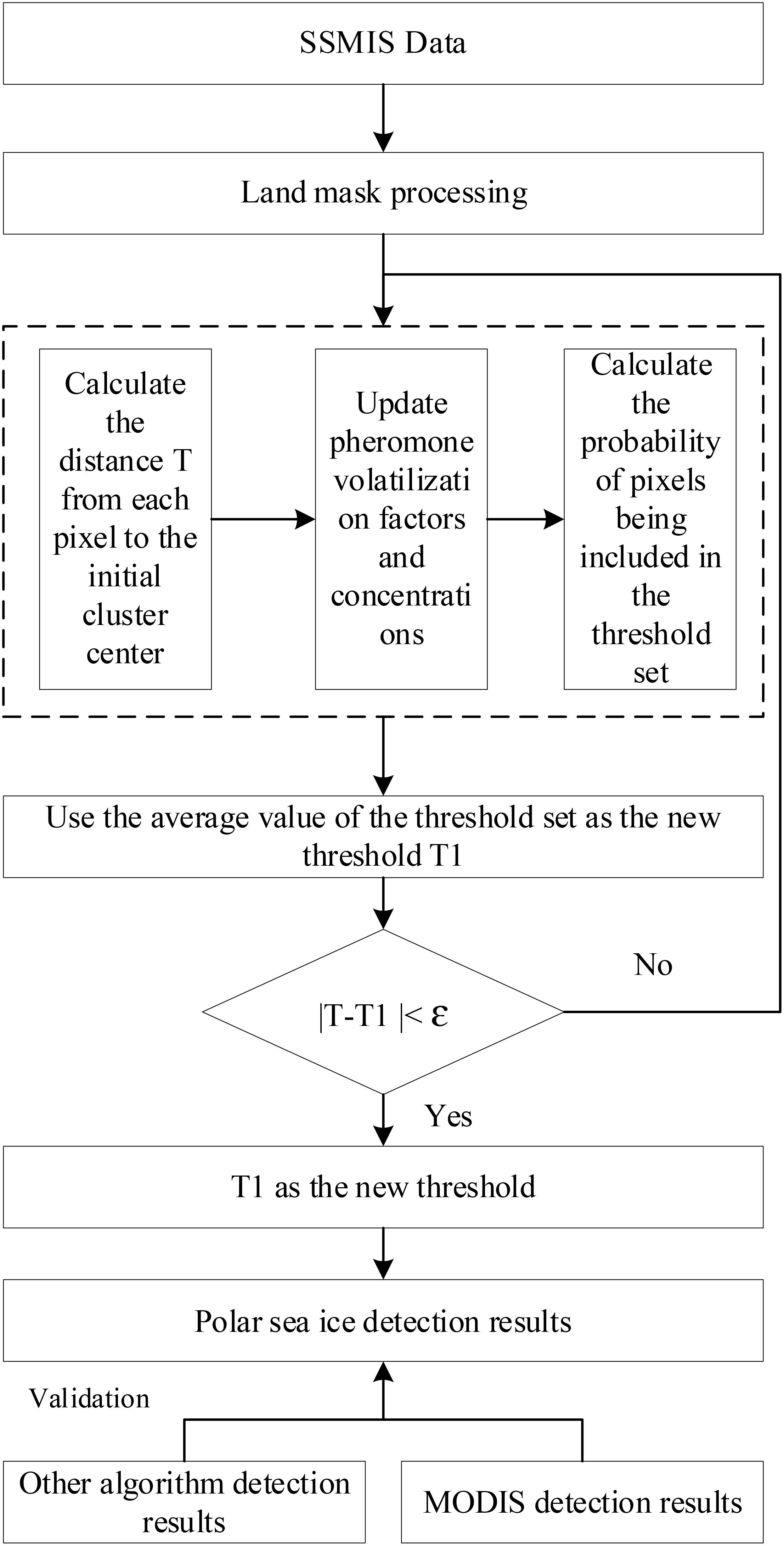
The ant colony algorithm adopts a positive feedback mechanism to continuously converge the search process and ultimately approach the optimal solution, making it easy to find the optimal segmentation threshold for seawater and sea ice. In addition, its self-organizing mechanism eliminates the need for the ant colony algorithm to have a comprehensive and detailed understanding of sea ice information. Therefore, the ant colony algorithm can be used for detecting sea ice distribution. However, the arbitrary selection of initial clustering centers and the fixed pheromone volatilization factor in the ant colony algorithm can lead to high computational complexity and susceptibility to local optima. In order to better apply the ant colony algorithm to sea ice distribution detection, this paper improved the initial clustering center selection and pheromone volatilization factor of the ant colony algorithm. And based on the Antarctic SSMIS 19.3GHz horizontal polarization bright temperature data during 2014-2024, the Antarctic sea ice distribution was obtained. The flow chart is shown in Figure 1.

Figure 1

Figure 1. Flow chart of sea ice detection based on the improved ant colony algorithm.

The steps of the improved ant colony algorithm in sea ice extraction are as follows.

1. Initialize threshold (Give the initial threshold of the ant colony algorithm, that is, select the initial clustering center.). The ants searching for food is the process of continuous clustering, and the clustering center is the food source that the ant colony algorithm is looking for (Yang and Hou, 2005). The ants walking in the ant colony algorithm is random, so giving the initial clustering center accurately and guiding the ants to go directly near the clustering center can greatly reduce the blindness of the search process, the computational load and speed up the clustering process. Unlike the traditional ant colony algorithms, this paper uses the data point with the highest mean dissimilarity as the initial clustering center for algorithm iteration. The calculation of mean anisotropy is shown in Equation 1. In addition, the cluster radius needs to be set, which determines the search range of the ants and the computational complexity of the algorithm. This paper gives a cluster radius of 20.

2. Calculate heuristic information η. The Euclidean distance d_i from each pixel to the initial threshold is calculated as follows.

$\begin{array}{ll}{\text{d}}_{\text{i}}=\sqrt{{({\text{X}}_{\text{i}}-\text{T})}^2}& (4)\end{array}$

which, X_i is the gray value of each pixel and T is the initial threshold or the threshold obtained by the last iteration.

Heuristic value is $\eta =\frac{1}{{\text{d}}_{\text{i}}}$. Heuristic value reflects the similarity between the pixel in the image and the clustering center. If the gray distance between the pixel and the clustering center becomes closer, d_i becomes smaller. With the increase of heuristic value, the similarity between the pixel and the clustering center increases.

3. Calculate the concentration of pheromones on each path. Update rules for pheromone is one of the core rules of the ant colony algorithm, and it also reflects the intelligence of the ant colony algorithm. The pheromone concentration is initialized before the first iteration, and the pixel values with Euclidean distance less than cluster radius r are assigned an initial pheromone concentration of 1, and the pixel values greater than r is 0. The initialization rules are as follows.

$\begin{array}{ll}{\text{Ph}}_{\text{i}}=\{\begin{array}{c}1\\ 0\end{array}\begin{array}{c}{\text{d}}_{\text{i}}\le \text{r}\\ {\text{d}}_{\text{i}}>r\end{array}& (5)\end{array}$

Starting from the second iteration, the formulas for calculating pheromone concentrations along each path are as follows.

$\begin{array}{ll}{\text{Ph}}_{\text{i}}(\text{t})=(1-\frac{n}{\text{m}}\text{ρ}){\text{ Ph}}_{\text{i}}(\text{t})+\rho \text{Δ}{\text{Ph}}_{\text{i}}& (6)\end{array}$

which, m and n are the number of rows and columns of the data, respectively, and $\text{ρ}$ is defined as the volatile variable of the pheromone over time, which represents the degree of attenuation of the pheromone over time. The larger the value is, the faster the attenuation is. If it is too large, it will easily cause premature convergence and fall into local optimum. To solve this problem, we combine Levy flight with the pheromone volatilization factor ρ, and as the algorithm continues to iterate, the pheromone volatilization factor ρ is constantly updated. The update of ρ is shown in Equations 2, 3. ΔPh_i is the increment of the pheromone in the last cycle and the current cycle, and the formula is as follows.

$\begin{array}{ll}\Delta {\text{Ph}}_{\text{i}}={\displaystyle {\sum }_{\text{k}=1}^{\text{n}}}\Delta {\text{Ph}}_{\text{i}}^k& (7)\end{array}$

4. Calculate the probability value Pi of each pixel into the threshold set. Equation 8 reflects the possibility that the gray-level of a pixel may be the best threshold in this iteration.

$\begin{array}{ll}{\text{P}}_{\text{i}}=\frac{{\text{Ph}}_{\text{i}}^{\alpha }(\text{t}){\eta }_{\text{i}}^{\beta }}{\sum {\text{Ph}}_{\text{i}}^{\alpha }(\text{t}){\eta }_{\text{i}}^{\beta }(\text{t})},j\in s& (8)\end{array}$

which, α is the heuristic factor of pheromone, which represents the importance of pheromone in algorithm iteration. The larger its value, the more the algorithm is affected by the pheromone. β is the heuristic factor of expectation, which represents the importance of path length in algorithm iteration. The larger its value, the more the algorithm is affected by the Euclidean distance. Here, we set the information heuristic factor α = 2 and heuristic factor β=4.

5. Determine whether P_i obtained in the previous step meets the iteration end condition. If the condition is met, the corresponding gray value is included in the threshold set, and then the threshold set is averaged to get a new threshold. If the conditions for the iteration end are met, the new threshold is output and the image is split, otherwise the second step is returned to continue the iteration. The conditions for the end of iteration of the algorithm is |T-T1|<ϵ. That is, if the threshold value obtained by this iteration is less than a certain range from that obtained by the last iteration, the threshold obtained by this iteration is considered to be the best global threshold.

6. The optimal threshold obtained in step (5) is used to classify sea ice and seawater.

7. To verify the feasibility and effectiveness of the proposed algorithm, we compared the sea ice distribution results obtained by the proposed algorithm with those of other algorithms and the results based on MODIS data. MODIS data determines sea ice based on the difference in reflectance between sea ice and seawater in the red and near-infrared bands. The specific formula is as follows.

$\begin{array}{ll}\{\begin{array}{c}Band1-Band2>a\\ Band1>b\end{array}& (9)\end{array}$

which, Band1 and Band2 are the reflectance values of MODIS bands 1 and 2, a=0.014 and b=0.067, respectively.

5 Results and verification

This paper used the improved ant colony algorithm to obtain the Antarctic sea ice distribution on January 9, 2018, as shown in Figure 2A. To verify the feasibility of the improved ant colony algorithm, we obtained the Antarctic sea ice distribution results on the same day based on iterative algorithm, maximum entropy algorithm, and basic global threshold algorithm, as shown in Figures 2B–D. From Figures 2A–D, it can be seen that the Antarctic sea ice spatial distribution obtained by the proposed algorithm, iterative algorithm, maximum entropy algorithm, and basic global threshold algorithm is basically consistent. To further verify the feasibility of the improved ant colony algorithm, this paper obtained the Antarctic sea ice distribution results from January 15, 2014 to January 15, 2024 based on the above four algorithms, and counted the number of sea ice pixels. The statistical results are shown in Figure 3. From Figure 3, it can be seen that the results of the above four algorithms are basically consistent. In summary, it is feasible to use the improved ant colony algorithm to detect the Antarctic sea ice distribution.

Figure 2

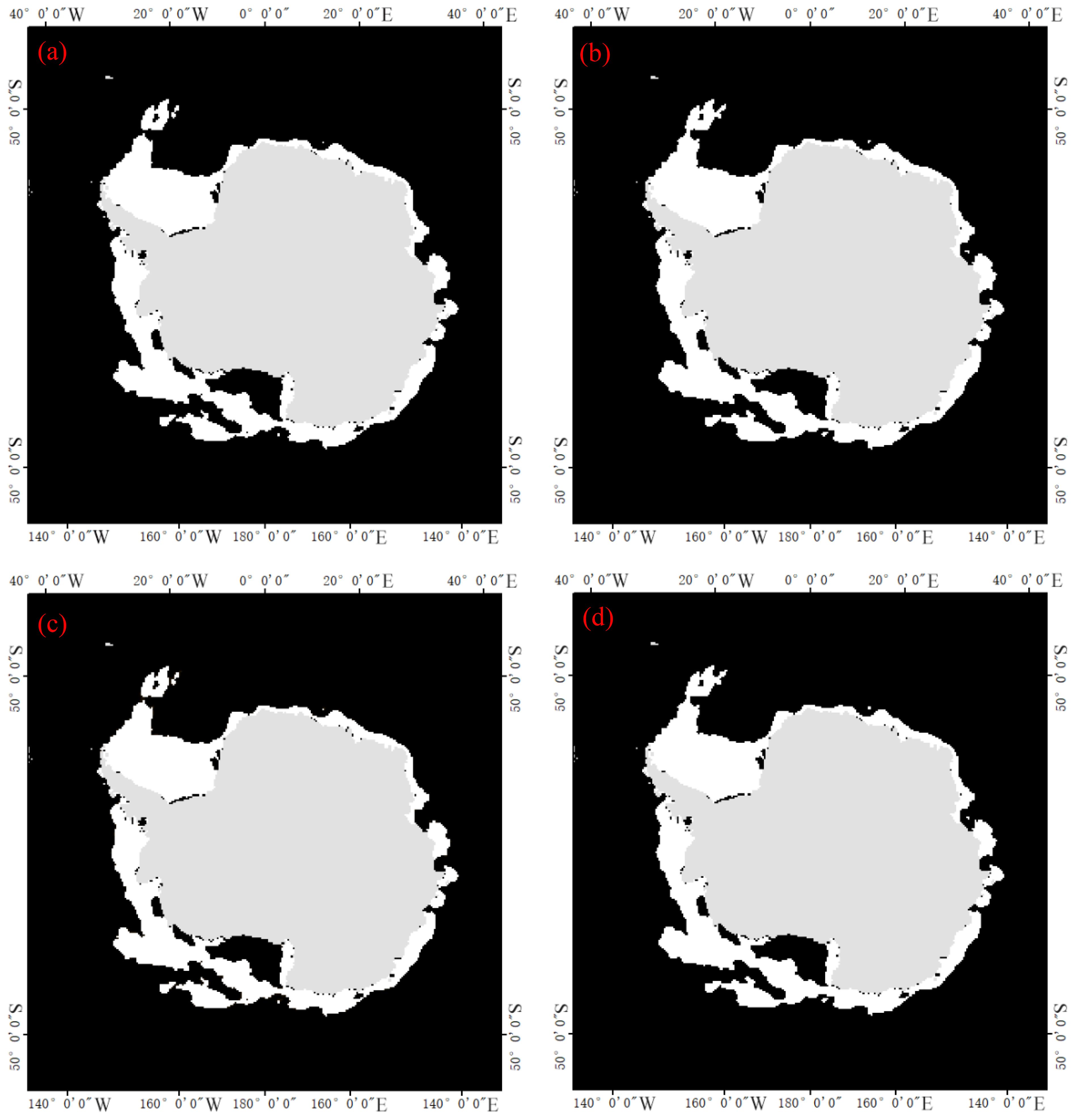
Figure 2. Results of different sea ice distribution detection algorithms (A) Improved ant colony algorithm, (B) Iterative algorithm, (C) Maximum entropy algorithm, (D) Basic global threshold algorithm (White represents sea ice regions, while black represents non sea ice regions).

Figure 3

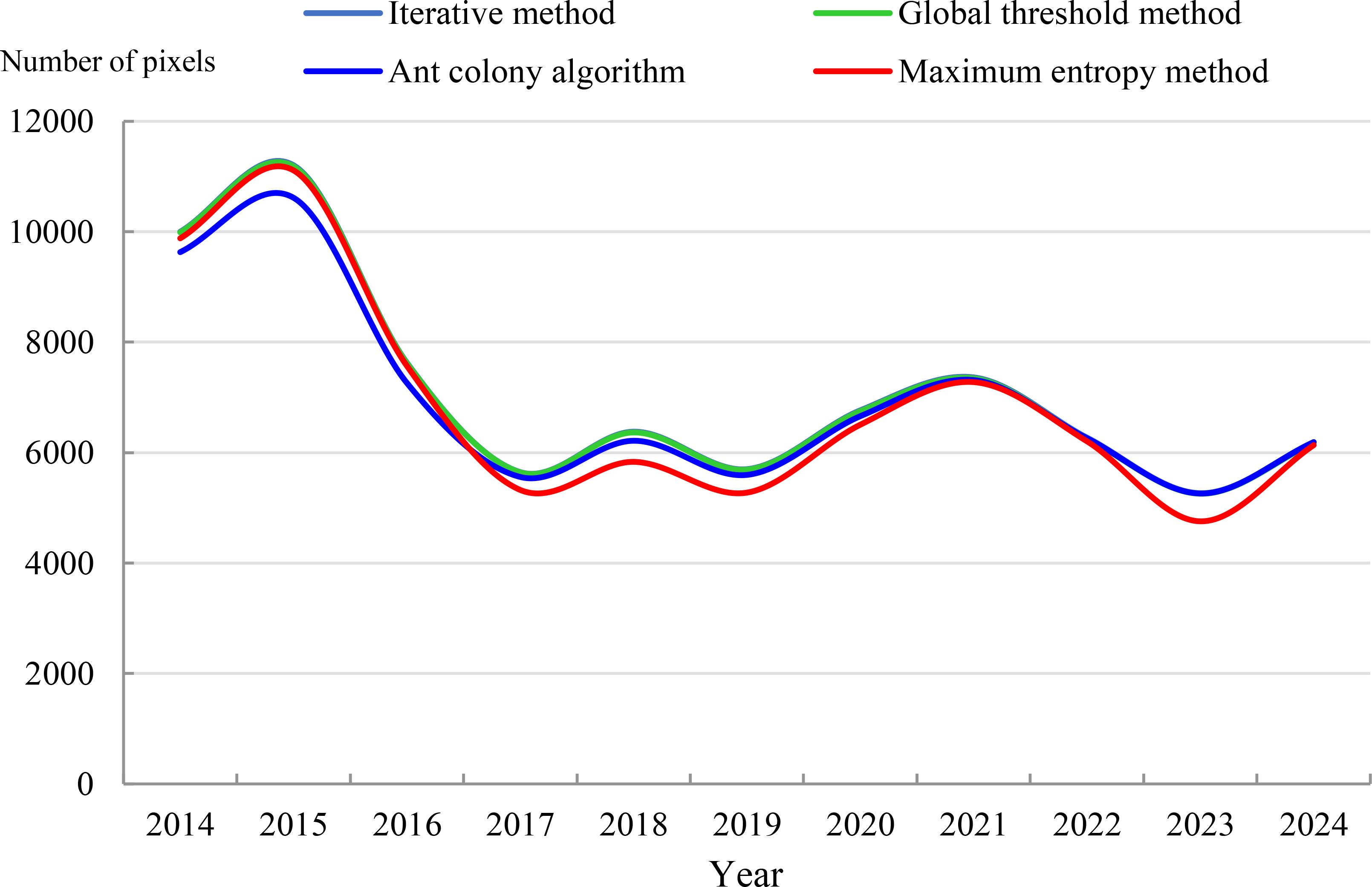
Figure 3. Statistical results of sea ice pixels based on proposed algorithm, iterative algorithm, maximum entropy algorithm, and basic global threshold algorithm.

In order to verify the high accuracy of the improved ant colony algorithm, this paper compared the sea ice distribution results obtained from MODIS data with the results obtained from the proposed algorithm, iterative algorithm, maximum entropy algorithm, and basic global threshold algorithm. The results are shown in Figures 4–6. Among them, the dates in Figures 4–6 are January 9, 2018, January 15, 2021, and January 15, 2024, respectively. From Figures 4–6, it can be seen that the sea ice distribution results are basically consistent in the most regions except for the red box.

Figure 4

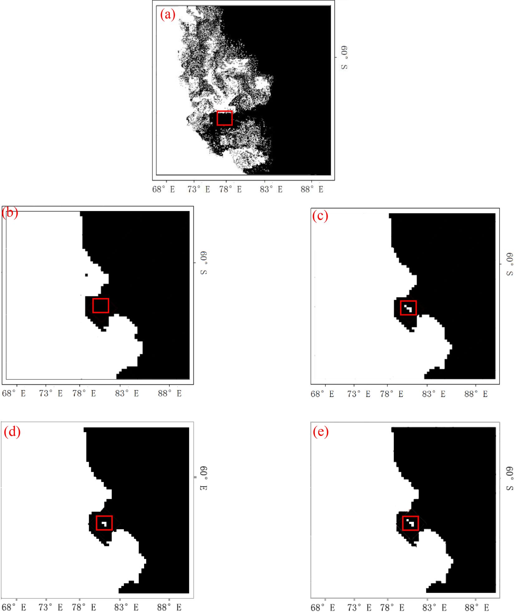
Figure 4. Sea ice distribution detection results on January 9, 2018 (A) MODIS data, (B) Improved ant colony algorithm, (C) Iterative algorithm, (D) Maximum entropy algorithm, (E) Basic global threshold algorithm (The white area is sea ice, and the black area is sea water).

Figure 5

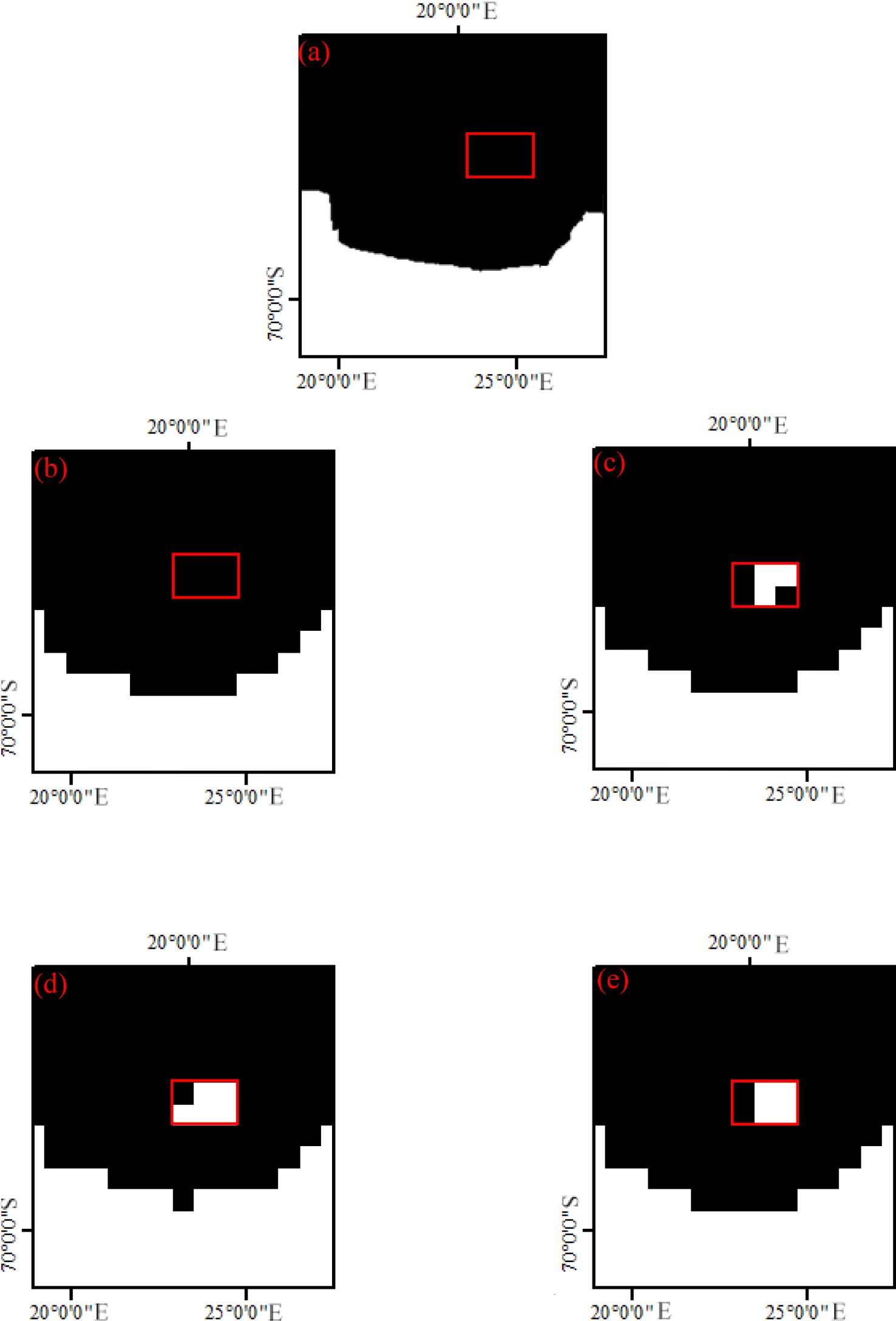
Figure 5. Sea ice distribution detection results on January 15, 2021 (A) MODIS data, (B) Improved ant colony algorithm, (C) Iterative algorithm, (D) Maximum entropy algorithm, (E) Basic global threshold algorithm (The white area is sea ice, and the black area is sea water).

Figure 6

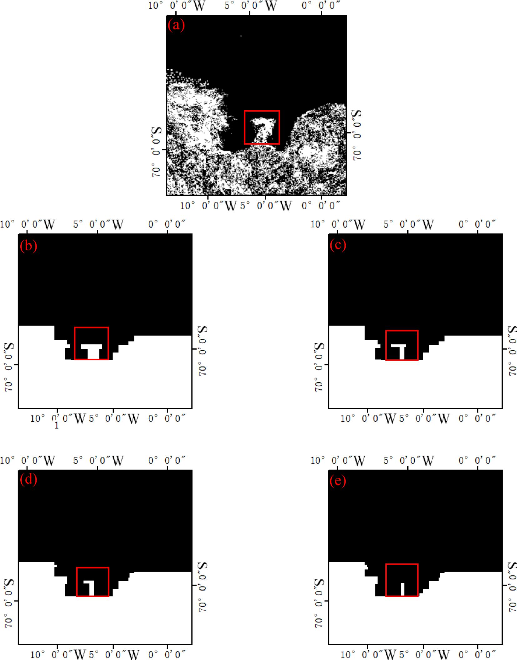
Figure 6. Sea ice distribution detection results on January 15, 2024 (A) MODIS data, (B) Improved ant colony algorithm, (C) Iterative algorithm, (D) Maximum entropy algorithm, (E) Basic global threshold algorithm (The white area is sea ice, and the black area is sea water.).

In order to further verify the accuracy of the improved ant colony algorithm, this paper used the sea ice distribution results obtained from MODIS data as the standard, and calculates the sea ice distribution detection accuracy for January 9, 2018, January 15, 2021, and January 15, 2022 based on the proposed algorithm, iterative algorithm, maximum entropy algorithm, and basic global threshold algorithm (Figures 4–6 only shows a partial display of these results). The results are shown in Table 1.

Table 1

Table 1. Sea ice detection accuracy of different algorithms.

From Table 1, it can be seen that the improved ant colony algorithm has the highest accuracy. The improved ant colony algorithm in the three selected regions in this paper has an average accuracy 4.99% higher than the iterative algorithm, 3.66% higher than the maximum entropy algorithm, and approximately 5.46% higher than the basic global threshold algorithm.

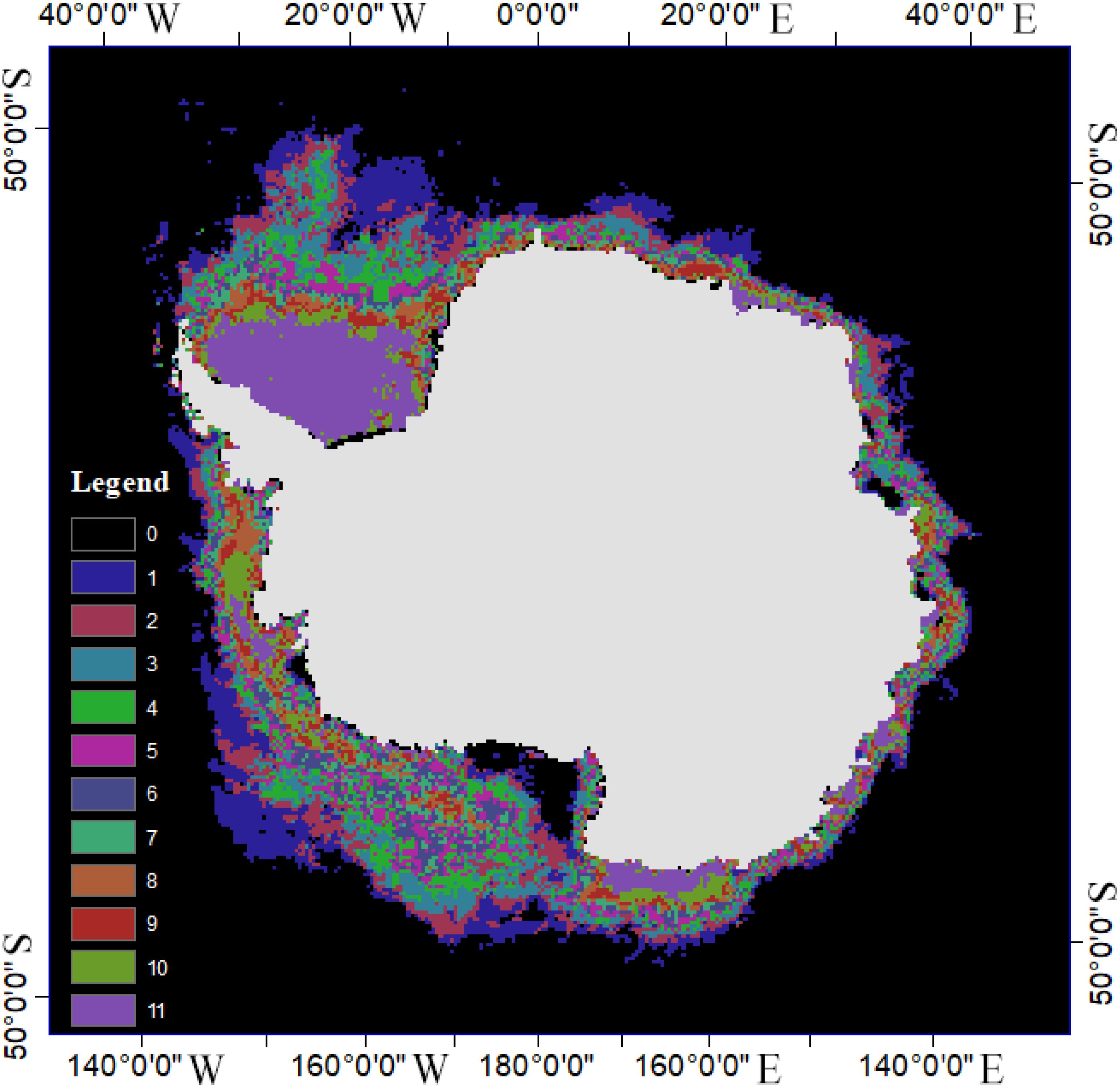
We used the improved ant colony algorithm to obtain a superimposed map of sea ice distribution from January 15, 2014 to January 15, 2024, as shown in Figure 7. From Figure 7, it can be seen that sea ice is mainly distributed around Antarctica, and the most stable sea ice regions are mainly distributed above the Antarctic Peninsula. The further away from Antarctica, the more unstable the sea ice state becomes.

Figure 7

Figure 7. Spatial changes of Antarctic sea ice distribution (Unit: days).

6 Discussion

The ant colony algorithm treats each pixel in remote sensing images as an ant. During the cyclic search process, the ants use pheromones with positive feedback characteristics as decision points, and model the pheromones left by each ant through the pheromone update mechanism. Then, from a global perspective, the algorithm calculates the probability of distance and path selection between each ant near the clustering center and the clustering center, and selects the optimal threshold for image segmentation after multiple cycles.

When using the ant colony algorithm to detect the Antarctic sea ice distribution, the initial clustering center selection of the ant colony algorithm is crucial. The initial clustering center selection of the traditional ant colony algorithm is arbitrary, which can lead to slow convergence speed of the algorithm, requires more iterations to find suitable solutions, which may cause the algorithm to fall into local optima rather than global optima. In this study, we used the point with the highest mean dissimilarity among the data points as the initial clustering center. Data points with high mean dissimilarity usually represent different regions of the data distribution, which makes the initial clustering centers we selected representative. This enables the algorithm to converge to a reasonable solution faster and reduces the deviation of the initial clustering centers, thereby reducing the risk of falling into local optima. In addition, the pheromone volatilization factor (ρ) of the traditional ant colony algorithms is fixed, which may result in the algorithm being unable to adapt to dynamic changes in different regions, which makes pheromone updates less flexible and the algorithm difficult to escape from local optima, and limits its ability to explore global optima. In this study, we combined Levy flight with pheromone volatilization factor, and as the algorithm iterates, the pheromone volatilization factor also changed accordingly. The dynamically updated the pheromone volatilization factor can better balance global and local search during the search process, improving the overall efficiency of the algorithm. Specifically, the updated pheromone volatilization factor can be adjusted according to the current search state, which makes the pheromone update more in line with the actual situation, and helps the algorithm converge to the global optimal solution faster, and dynamically adjusting pheromone volatilization factor can prevent pheromones from prematurely concentrating on the local optimal solutions, thereby increasing the chance of escaping from local optima. We compared the sea ice detection results obtained based on the improved ant colony algorithm with those of other algorithms, and the results showed that the proposed algorithm achieved the higher accuracy in sea ice detection.

However, there are still some shortcomings in this study that (1) Due to the scarcity of on-site data in polar regions, MODIS data was used in this paper to verify the accuracy of the proposed algorithm. However, optical data is susceptible to interference from clouds and fog, which limits the verification regions. (2) There is a time difference in the acquisition of SSMIS data and MODIS data, which may lead to errors in the sea ice distribution results obtained from the two types of data. In future study will consider combining on-site data and SAR data for more comprehensive validation. (3) Although selecting the point with the highest average dissimilarity can increase the diversity of initial centers, the presence of noise or outliers in the data may still result in the initial clustering centers being unrepresentative, thereby affecting the final clustering results. (4) The improved ant colony algorithm only extracts the sea ice distribution information and cannot obtain the one-year ice and multi-year ice distribution information.

7 Conclusion

This paper improved the ant colony algorithm by accurately setting the clustering center and dynamically updating the global pheromone concentration, and utilized its ability to find the shortest path for optimization. The threshold for sea ice distribution detection is regarded as the optimal solution to the problem, and a sea ice distribution detection method based on the improved ant colony algorithm is proposed. Compare the sea ice detection results obtained by the proposed algorithm in this paper with those obtained by the iteration algorithm, maximum entropy algorithm, and basic global threshold algorithm, and validate them with MODIS data. The results indicate that the proposed algorithm detects the least number of sea ice pixels and produces the most accurate results. The detection method can also be applied to other sea regions, which provides methodological support for the sea ice distribution detection based on microwave radiometer data.

Data availability statement

The original contributions presented in the study are included in the article/supplementary material. Further inquiries can be directed to the corresponding author/s.

Author contributions

XW: Conceptualization, Data curation, Funding acquisition, Methodology, Supervision, Validation, Visualization, Writing – original draft, Writing – review & editing. ZS: Data curation, Formal analysis, Methodology, Resources, Validation, Visualization, Writing – original draft, Writing – review & editing.

Funding

The author(s) declare financial support was received for the research, authorship, and/or publication of this article. This research was supported by the Key Laboratory of Grain Information Processing and Control (Henan University of Technology), Ministry of Education under Grant KFJJ-2020-113.

Conflict of interest

The authors declare that the research was conducted in the absence of any commercial or financial relationships that could be construed as a potential conflict of interest.

Generative AI statement

The authors declare that no Generative AI was used in the creation of this manuscript.

Publisher’s note

All claims expressed in this article are solely those of the authors and do not necessarily represent those of their affiliated organizations, or those of the publisher, the editors and the reviewers. Any product that may be evaluated in this article, or claim that may be made by its manufacturer, is not guaranteed or endorsed by the publisher.

References

Cavalieri D. J., Parkinson C. L. (2012). Arctic sea ice variability and tread -2010. Cryosphere 6, 881–889. doi: 10.5194/tc-6-881-2012

Crossref Full Text | Google Scholar

David L. (2016). Multiyear arctic ice classification using ASCAT and SSMIS. Remote Sens. 8, 294–294. doi: 10.3390/rs8040294

Crossref Full Text | Google Scholar

Dawoud A., Netchaev A. (2012). Preserving objects in Markov random fields region growing image segmentation. Pattern Anal. Appl. 15, 155–161. doi: 10.1007/s10044-011-0198-x

Crossref Full Text | Google Scholar

Dorigo M., Maniezzo V., Colorni A. (1996). Ant System: Optimization by a colony of cooperating agents. IEEE Trans. Syst. Man Cybernetics - Part B. IEEE Trans. On Cybernetics 26, 29–41. doi: 10.1109/3477.484436

PubMed Abstract | Crossref Full Text | Google Scholar

Duspayev A., Flanner M. G., Riihelä A. (2024). Earth’s sea ice radiative effect from 1980 to 2023. Geophysical Res. Lett. 51, e2024GL109608. doi: 10.1029/2024GL109608

Crossref Full Text | Google Scholar

Haverkamp D., Soh L. K., Tsatsoulis C. (1993). “A dynamic local thresholding technique for sea ice classification,” in Proceedings of IGARSS '93 - IEEE International Geoscience and Remote Sensing Symposium. (Tokyo, Japan). 2, 638–640. doi: 10.1109/IGARSS.1993.322252

Crossref Full Text | Google Scholar

Kern S. (2004). A new method for medium-resolution sea ice analysis using weather-influence corrected Special Sensor Microwave/Imager 85 GHz data. Int. J. Remote Sens. 25, 4555–4582. doi: 10.1080/01431160410001698898

Crossref Full Text | Google Scholar

Leigh S., Wang Z., Clausi D. A. (2013). Automated ice—Water classification using dual polarization SAR satellite imagery. IEEE Trans. Geosci. Remote Sens. 52, 5529–5539. doi: 10.1109/TGRS.2013.2290231

Crossref Full Text | Google Scholar

Li X. (2005). On the MODIS data and its application tosensitivity analysis between land coverchange and climatic factor in Arid Area (Xinjiang, China: Xinjiang University).

Google Scholar

Liu H., Guo H., Zhang L. (2015). SVM-based sea ice classification using textural features and concentration from RADARSAT-2 dual-pol scan SAR data. IEEE J. Selected Topics Appl. Earth Observations Remote Sens. 8, 1601–1613. doi: 10.1109/JSTARS.2014.2365215

Crossref Full Text | Google Scholar

Piñones A., Aziares-Aguayo N., Amador-Véliz P., Mercado-Peña O., González-Reyes A., Valdivia N., et al. (2024). Local and remote atmosphere-ocean coupling during extreme warming events impacting subsurface ocean temperature in an Antarctic embayment. J. Geophysical Research: Oceans 129, e2023JC020735. doi: 10.1029/2023jc020735

Crossref Full Text | Google Scholar

Spreen G., Kaleschke L., Heygster G. (2008). Sea ice remote sensing using AMSR-E 89-GHz channels. J. Geophys. Res. 113, C02S03. doi: 10.1029/2005JC003384

Crossref Full Text | Google Scholar

Tan W., Li J., Xu L., Chapman M. A. (2018). Semiautomated segmentation of sentinel-1 SAR imagery for mapping sea ice in labrador coast. IEEE J. Selected Topics Appl. Earth Observations Remote Sens. 11 (5), 1419–1432. doi: 10.1109/JSTARS.2018.2806640

Crossref Full Text | Google Scholar

Tikhonov V. V., Repina I. A., Raev M. D., Sharkov E. A., Ivanov V. V., Boyarskii D. A., et al. (2015). A physical algorithm to measure sea ice concentration from passive microwave remote sensing data. Adv. Space Res. 56, 1578–1589. doi: 10.1016/j.asr.2015.07.009

Crossref Full Text | Google Scholar

Wang J. F., Massonnet F. I. A., Goosse H., Luo H., Barthelemy A., Yang Q. H. (2024). Synergistic atmosphere-ocean-ice influences have driven the 2023 all-time Antarctic sea-ice record low. Commun. Earth Environ. 5, 415. doi: 10.1038/s43247-024-01523-3

Crossref Full Text | Google Scholar

Wen L. (2004). “An efficient algorithm for mining frequent closed itemset,” in Fifth World Congress on Intelligent Control and Automation (IEEE Cat. No.04EX788). (Hangzhou, China). 5, 4296–4299. doi: 10.1109/WCICA.2004.1342322

Crossref Full Text | Google Scholar

Yang H. F., Hou C. Z. (2005). Image segmentation by ant colony algorithrn based on two-dimensional gray. Laser& Infrared 35, 614–6l7. Available online at: https://www.semanticscholar.org/paper/Image-Segmentation-by-Ant-Colony-Algorithm-Based-on-Hai-feng/de010e2f8fd69d14341612571456f8b0a465763f.

Google Scholar

Yang X., Clausi D. A. (2012). Evaluating SAR sea ice image segmentation using edge-preserving region-based MRFs. IEEE J. Selected Topics Appl. Earth Observations Remote Sens. 5 (5), 1383–1393. doi: 10.1109/JSTARS.2012.2217940

Crossref Full Text | Google Scholar

Yu Q., Clausi D. (2008). IRGS: image segmentation using edge penalties and region growing. Pattern Anal. Mach. Intelligence IEEE Trans. 30, 2126–2139. doi: 10.1109/TPAMI.2008.15

PubMed Abstract | Crossref Full Text | Google Scholar

Zakhvatkina N. Y., Alexandrov V. Y., Goosse H., Johannessen O. M., Sandven S., Frolov I. Y. (2013). Classification of sea ice types in ENVISAT synthetic aperture radar images. IEEE Trans. Geosci. Remote Sens. 51, 2587–2600. doi: 10.1109/TGRS.2012.2212445

Crossref Full Text | Google Scholar

Zakhvatkina N., Korosov A., Muckenhuber S., Sandven S., Babiker M. (2017). Operational algorithm for ice-water classification on dual-polarized RADARSAT-2 images. Cryosphere 11, 33–46. doi: 10.5194/tc-11-33-2017

Crossref Full Text | Google Scholar

Zhang X., Deser C. (2024). Tropical and Antarctic sea ice impacts of observed Southern Ocean warming and cooling trends since 1949. NPJ Clim Atmos Sci. 7, 197. doi: 10.1038/s41612-024-00735-w

Crossref Full Text | Google Scholar

Zhang X. L., Yan H. Y., Xu Q. J. (2016). Threshold medical image segmentation based on improved ant colony algorithm. J. Beijing Jiaotong Univ. 40, 40–44. doi: 10.1007/s11227-018-2622-0

Crossref Full Text | Google Scholar

Zhao X., Chen Y., Kern S., Qu M., Ji Q., Fan P., et al. (2021). Sea ice concentration derived from FY-3D MWRI and its accuracy assessment. IEEE Trans. Geosci. Remote Sens. 60, 1–18. doi: 10.1109/TGRS.36

Crossref Full Text | Google Scholar