Optimising the design and analysis of capture-mark-recapture experiments using individual-based models

Capture-mark-recapture methods (CMR) are a commonly used tool in species conservation and management for the estimation of demographic parameters in a population. However, biases in these estimates can occur due to the heterogeneity in processes influencing recapture data or the experimental design. We outline an approach to quantify and identify ways to reduce this bias through both experimental design and data analysis, using individual based modelling (IBMs). By using an IBM that includes key sources of heterogeneity that are believed to exist in the system, the release and recapture of marked individuals can be simulated under differing experimental, behavioural or landscape scenarios. Using this IBM as a data-generator, we compare a simulated population of individuals with a subset of that population that represent those marked and recaptured in a CMR experiment. Parameter estimates from the data generated by the marked subset are then compared to ‘true’, realised parameters from the wider, unmarked population. We demonstrate this with an application of ‘simulated tagging’ of Pacific skipjack tuna (Katsuwonus pelamis), using scenarios of different release locations of marked individuals, alternative band-recovery models, and differing assumptions that define the spatial extent of the unmarked population. We quantify the error in the estimated survival and fishing mortality parameters and examine how these can be reduced by following differing release and analysis strategies. We show that spatiotemporal heterogeneity of individual dispersion and recovery effort (i.e. fishing pressure) led to severe bias in recapture probability estimates, up to 361%, regardless of experimental design. However, when the baseline of the unmarked population of which marked animals were assumed to be representative was defined by spatial coverage of recaptures, rather than a fixed, spatial management area, bias was reduced to 25%. Our results show that the use of IBM frameworks exploring alternative hypotheses, either in the design of or post-hoc analyses of CMR experiments, support maximising the information that can be derived and quantify the degree of potential bias due to analysis model mis-specification. Furthermore, these methods can benefit other sampling and monitoring programmes in systems with high levels of spatial or ecological heterogeneity.

1 Introduction

A significant challenge in ecology is to infer population processes from a limited subset of individuals that can be sampled (Tourani, 2022). In the case of widely or heterogeneously distributed species, the representativeness of the subset observed from a particular sampling strategy can be highly questionable (Rees et al., 2011; Kolody and Hoyle, 2015). Marking and tracking animals, using Capture-Mark-Recapture (CMR) experiments, is a commonly applied methodology in ecological research and management. CMR provides a means of monitoring animal populations and estimating demographic parameters such as population size, distribution and rates of mortality, growth, and connectivity (Wang et al., 1995; Pine et al., 2003; Pollock et al., 2004; Sippel et al., 2014). In a CMR experiment, a subset of the population in a region is marked, of which the number of individuals, key biological properties and release locations are known. This group can then be monitored through time via future encounters of the marked individuals when sampling the population, and demographic or life history parameters of that population are then estimated (Lindberg and Rexstad, 2001; Sandercock, 2006).

The assumptions of the CMR analytical model chosen to estimate parameters greatly influence the resulting bias in these estimates. A critical assumption in such models is that the marked subset is representative of the unmarked population of interest and key for the accuracy of these estimations (Lindberg and Rexstad, 2001; Pine et al., 2003). Failure to satisfy this assumption in subsequent analyses, or account for their potential effects, may lead to a bias in population level parameter estimations (Pledger and Efford, 1998; Pledger, 2005; Mathur, 2007; Fletcher et al., 2012; Abadi et al., 2013; Guillemain et al., 2014).

CMR experiments aiming to estimate or inform population dynamics parameters would ideally mark individuals by random sampling of the studied population. However, in the case of heterogeneously and/or widely distributed species this is often logistically challenging, and so typically animals are marked in a small number of spatially-limited locations, from which they move through the region of interest and mix with the unmarked population. Over some initial period of time, ideally the marked animals will become distributed relative to the distribution of the unmarked population, such that random sampling any set of animals in the population will lead to the same probability of recaptures with marked individuals. As recaptures can occur immediately after release, spreading marked individuals across many locations and times may help achieve mixing more quickly, improving the representativeness of the marked subset and subsequent estimation of population parameters. However, attempts to quantify the reliability of this mixing have generally concluded that the underlying heterogeneity in the processes driving behaviour, recapture effort and the spatial extent of the population, likely make the degree of representation by marked individuals highly variable in both space and time (Pépino et al., 2012, 2016; Schaub and Royle, 2014; Sippel et al., 2014; Kolody and Hoyle, 2015; Chadœuf et al., 2018; Moqanaki et al., 2021).

Testing analytical models using data generated by simulation modelling provides a way to examine the bias in estimated life history parameters resulting from such violation of sample design (Rees et al., 2011; Abadi et al., 2013). Individual-based simulation models (IBMs) offer the benefit of being structured on the fundamental unit of the individual, as are CMR experiments themselves. This allows population-level parameters such as movement rates, mortality or probability of detection to emerge from the simulation of large numbers of animals, rather than being explicitly defined (Grimm and Railsback, 2005; Vangestel et al., 2011; Meli et al., 2013). Simulated individuals can have unique properties, such as age or sex, and have variable and stochastic behavioural responses to a spatiotemporally heterogeneous habitat. In contrast to Eulerian or state variable models of animal population dynamics, the pathways and properties of many individuals can be tracked, providing a measure of cumulative process effects through time experienced by individuals and the variability of these effects across groups of individuals.

Generating data using an IBM that contains spatial and temporal heterogeneity in the processes hypothesised to violate the assumptions of the analytical model can be used to quantify the degree of the bias that may arise under a particular experiment-analysis design. By simulating the release and subsequent recapture over time of marked, free-roaming individuals released in discrete locations, parameters estimated from these data by a proposed analytical model can be compared to realised values from the same or a parallel simulation of individuals from an unmarked population throughout the management region of interest. While goodness-of-fit tests can be applied to the results of a particular analytical model using real data, bias due to model mis-specification and failure to satisfy assumptions requires full knowledge of the underlying system, typically only available through simulation.

Here, we demonstrate this approach with an example application for a widely-distributed, highly mobile species, skipjack tuna (Katsuwonus pelamis). This species challenges traditional CMR analytical methods as their dynamics are driven by highly heterogeneous spatiotemporal ocean habitats, and recapture of marked individuals relies on non-uniform recovery effort and reporting from commercial fisheries across large regions defined by population dynamics models used in stock assessment. This frequently results in a large variability in recapture rates, due to the highly dynamic spatiotemporal nature of fishing effort, and the degree to which ‘tagged’ individuals in these CMR experiments mix with and represent the underlying population in an assessment region has been frequently questioned (Kolody and Hoyle, 2015; Peatman et al., 2022).

We combine simulations from an IBM parameterised for this species to generate data with two formulations of a simple Brownie ‘band-recovery’ analysis (Brownie, 1978a), a typical analytical model used to inform time dependant natural and fishing mortality estimations in fish species (Lauretta and Goethel, 2017; Peatman et al., 2022; Vincent and Pilling, 2023), using two model parameters: survival and recapture probability, respectively. These Brownie models require several assumptions to be met. First, the marked population should be a representative sample of the population of interest on which the analysis is structured. Second, that survival and recapture probability parameters are age-independent, that is, they do not change for individuals of differing ages or within some age structure. Finally, while these parameters can change through time, they are assumed to be shared by all individuals in the population of interest during each time-period. In the case of CMR experiments on skipjack tuna, heterogeneity in distribution, heterogenous recovery effort and ontogenetic influences in survival and vulnerability to fishing gears results in all the above assumptions being violated. However, our hypothesis testing exercise permits quantification of the resulting parameter bias under differing experimental designs or complexity in this family of models.

In our example, first we test differing strategies for the spatial spread of release locations for their ability to improve the representativeness of the marked population with the population of interest. Secondly, we use alternative formulations of our Brownie analytical model which better account for the spatiotemporal heterogeneity in recovery effort. Finally, we can also test how parameter bias is influenced by the lack for spatial coverage of marked individuals within a widely-distributed unmarked population, and how this bias can be reduced through redefining the spatial extent of what can be assumed to be an appropriate study population of interest. By defining this spatial extent as a function of the spread and recapture of marked individuals themselves, rather than a fixed region based on management objectives, our approach can quantify the spatial area over which a given parameter precision can be expected.

We use simulation experiments under these three types of scenarios to illustrate how simulated data from IBMs can be used to guide the spatial design of such CMR experiments, as well as the choice of procedures used to analyse their resulting data.

2 Methods

2.1 Method summary

Our approach consists of the following steps:

1. Use a simulation model as a data generator, parameterised for the heterogeneous processes (such as spatiotemporal differences in environment, food availability, or predation/exploitation) believed to influence the movement, recapture and other properties of interest in the population.

2. Simulate the population, including both marked and unmarked individuals, and track their properties over time, generating recapture data from the marked group as a function of their individual pathways, survival, and recapture effort.

3. Calculate the realised ‘true’ parameter values for the processes of interest from the unmarked population. These are then compared to those same parameters as estimated from the recapture data simulated by the marked population, using the analytical methods being considered for the CMR experiment data (in our example case, a Brownie band-recovery model), to quantify the bias in parameter estimates.

4. Repeat steps 2 and 3, examining alternative experimental designs and analytical assumptions of the mark-release effort strategy for their impact on this parameter estimate bias.

For our example application, we simulate marked and unmarked Pacific skipjack tuna under different CMR design-analysis scenarios, using recapture probabilities that emerge across a group of individuals to generate recapture matrices for the estimation of demographic parameters.

2.2 Simulation model

We use an existing individual-based simulation model, Ikamoana (Scutt Phillips et al., 2018), to simulate movement of our target species. The model uses Lagrangian formulations of Eulerian advection-diffusion equations, building on the Parcels particle simulation engine (Delandmeter and van Sebille, 2019) to simulate fish movement behaviours. Individual particles representing animals perform three types of movements: passive transport by ocean currents, active movements towards preferred habitats, and random movements that mimic the search strategies of fish. These movement behaviours are driven by heterogeneous environmental and habitat fields, with advection-diffusion parameters estimated for Pacific skipjack tuna externally in a Eulerian ecosystem model (SEAPODYM, Senina et al., 2020). The positions, internal states such as age, and the history of individuals are recorded along their pathways. A full description of this simulation model is given in Scutt Phillips et al. (2018), and the base code is publicly available online (https://github.com/PacificCommunity/OFP-Ikamoana).

In tuna CMR ‘tagging’ experiments, recapture of marked individuals is carried out by commercial and recreational fishers, resulting in dead-recoveries. We therefore introduce a new probabilistic mechanism of natural and fishing mortality to the Ikamoana model to derive the survival and recapture probability of individuals. This allows tracking of the recovery probability that emerges as a function of each individual fish’s movement through spatiotemporally varying fields of historical fishing mortality, as estimated from catch and effort data in SEAPODYM (Senina et al., 2020).

To calculate the effect of spatially varying fishing mortality in a Lagrangian context, we must incorporate values normally considered as deterministic reduction of the number or biomass of animals within an area over a timestep. Instead, we consider these values as a probabilistic function of dying for an individual within the area, assuming that the probability that an individual is caught is uniform across all the individuals present in that area.

Rather than a proportion of all individual particles being removed from the simulation over time to represent mortality, instead each n-th individual has a probability of survival s_n which diminishes over time due to either natural or fishing mortality. Therefore, the population size represented by any group of particles is given by the sum of all survival probabilities in the group. By maintaining all the particles in the simulation, we increase the spatiotemporal sampling of our model domain, so can base our results on larger sample sizes.

Our model domain is divided into a regular grid of resolution ¼° x ¼°, and the total reduction in biomass in each grid cell at time t, emerges from the cumulative probability of each n-th individual dying of natural causes or being caught with probability m_n(t) or h_n(t), respectively, depending on the observed spatial and temporal distribution of fishing effort and/or catch by fishery in that cell. For each position x and time t, the instantaneous mortality rate over time-step Δt in that cell, Z(x,t), causes a proportion of fish there present to be depleted through the combined effects of fishing and natural mortality, F(x,t) and M(x,t), respectively. For the definition and estimation of these parameters, we refer the reader to SEAPODYM (Senina et al., 2020).

The probability of any individual dying at position x at time t, z(x,t), is therefore simply m(x,t) + h(x,t), and can be defined as a Lagrangian reinterpretation of the death rate from the Baranov catch equation (Baranov, 1918), a common model for estimating removal of animal biomass in fisheries applications.

$\begin{array}{ll}z(x,t)=1-e^{-Z(\text{x},\text{t})}& (1)\end{array}$

Here, instantaneous mortality affects the probability of any individual surviving, rather than the removal of a number of individuals passing through position x at time t. However, consecutive values of z(x,t) over time do not independently influence the survival of an individual n over time, as death can only occur once. For a given time representing an individual ‘proper’ time-at-liberty τ, which is some time interval from its time of release t₀ and time-step t_k, the probability that the n-th individual survives this interval, S_n(τ), is simply the product of all probabilities of n having not died during t = t₀ to t = t_k.

$\begin{array}{ll}{s}_n(\tau )=\prod _{i=t_0}^{t_k}(1-z(x_i,t_i)), \tau =t_k-t_0& (2)\end{array}$

These probabilities are recorded along the trajectory of all individuals through each simulation, their values changing in response to the cumulative effect of the individual’s position, age, and decreasing chance of survival throughout its time-at-liberty τ.

In the context of recapture/encounter probability of marked individuals in our tag recovery application for skipjack tuna, probability of an individual’s death due to fishing is also that of tag recapture, assuming 100% reporting of tags post capture. This probability of recapture at a particular location x and time t, h(x,t), is the proportion of total instantaneous mortality Z(x,t) caused by fishing at time t at x.

$\begin{array}{ll}h(x,t)=\frac{F(x,t)}{Z(x,t)}z(x,t)& (3)\end{array}$

Substituting (1) into Equation 3, we recover an analogy of the Baranov catch equation (Baranov, 1918).

Thus, the overall probability of a recapture for an individual n during an arbitrary time interval of length j > Δt during it’s time at liberty, is simply the sum of all probabilities of having survived until the time prior to recapture (Equation 2) and then having been caught (Equation 3) during each time during the interval (t_k, t_k+Δj).

$\begin{array}{ll}{p}_n(j)={\displaystyle \sum _{i=t_k}^{t_k+\text{Δ}j}}(s_n(i-1)·h(x_i,t_i)) \forall i\in (t_k,t_k+\text{Δ}j)& (4)\end{array}$

In our model, where individuals are recovered dead, this probability of recapture at an individual level will necessarily asymptote with increasing individual time-at-liberty τ, as additional exposure of an individual to recovery effort will result in decreasing chance of recapture due to the preceding natural mortality, and fishing mortality associated with past effort. An individual movement trajectory from Ikamoana is given in Figure 1, demonstrating how movement through a heterogeneous field of fishing mortality influences survival and recapture probability over time. Using this individual-level and probabilistic approach to generate a recapture probabilities through time, it is then straightforward to generate simulated recapture data over a given time window.

Figure 1

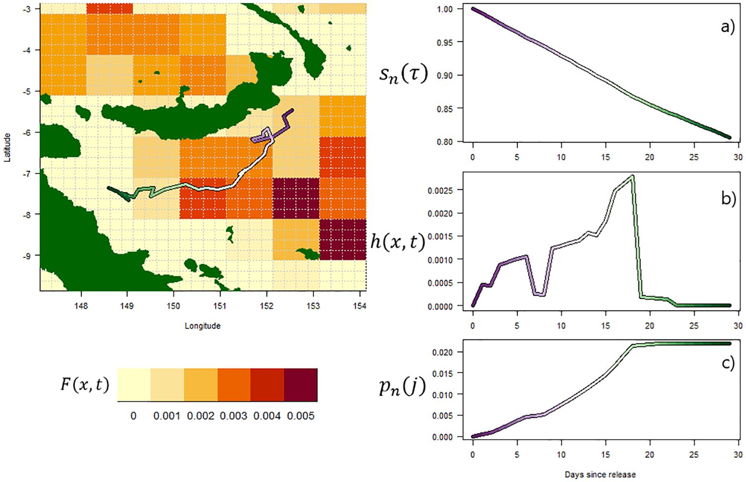
Figure 1. Left: Diagram of an individual pathway in Ikamoana, over an example field of spatially heterogeneous fishing mortality (high mortality in red, low in yellow). Right: corresponding time-series along this pathway of, from top to bottom, (A) survival after time-at-liberty τ, s_n(τ); (B) probability of death due to fishing at time t, h(x,t); and (C) cumulative recapture probability after time-at-liberty τ, P_n(τ).

2.3 Simulation experiments

CMR experiments have been a feature of the monitoring program for skipjack in the western and central Pacific Ocean (WCPO) since the 1970s with the subsequent CMR data used in tag attrition models (Kleiber et al., 1987), integrated stock assessments (Hampton and Fournier, 2001) and ecosystem models (Senina et al., 2020). Annual or biannual CMR ‘tagging’ campaigns in the WCPO have now been undertaken since 2006 as part of the Pacific Tuna Tagging Project (PTTP Leroy et al., 2013).

In our example application, we have chosen an important management region within the WCPO convention area for tuna fisheries, the archipelagic area around the Solomon Islands and Papua New Guinea. This area is centred in the core of Pacific skipjack tuna habitat (Senina et al., 2020), constitutes a major proportion of catch from the WCPO convention area (Hare et al., 2021), and forms a distinct region within the population dynamics models currently used to manage WCPO tunas (Castillo-Jordan et al., 2022). As with many CMR programmes, much of the experimental design of fish tagging in this region is largely determined by logistical constraints.

We simulated a year of continuous, monthly CMR experiments using multiple combinations of release locations, and estimated survival and fishing mortality parameters using a simple Brownie band-recovery model from the generated recapture data (Brownie, 1978b). We compare these parameter estimates to ‘true’, realised survival and fishing mortality parameters from a simulated, unmarked population whose initial positions are spread throughout a surrounding region defined by differing conditions, at the same moment as each release experiment.

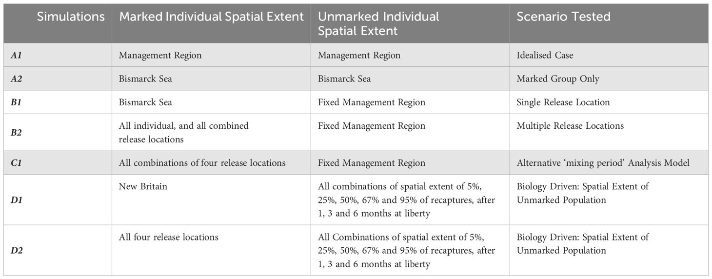
Our simulation experiments test combinations of three experiment-analysis designs. The full list of simulation experiments performed is given in Table 1.

1. We vary the spatial extent of marked individual releases (‘release locations’) from which parameters will be estimated, comparing them to unmarked individuals within a pre-defined management area.

2. We then test varying the analysis method for estimating the demographic parameters from the marked population, accounting for the period during which individuals ‘mix’ with the unmarked population from the pre-defined management area.

3. Finally, we vary the spatial extent of the unmarked population from which realised parameters are calculated, using a more biologically meaningful definition that emerges from the spatial distribution of recaptures, and to which CMR estimated parameters will be compared.

Table 1

Table 1. List of simulation CMR experiments for our example application on Pacific skipjack tuna.

Each time marked individuals were released at a particular location, 100,000 individuals were simulated to adequately sample the space of potential movement trajectories post marking, as a function of the movement model. For each experiment, individuals were released throughout a 1°x1° area at locations within a currently assumed spatial management region for this species and corresponding to four areas of historical high tag releases: the Bismarck Sea, south of New Britain, north of Isabel, and the New Georgia Sound (‘The Slot’). We also simulated an ‘idealised’ release, by assuming that marked individuals could be released throughout the management region in proportion to the unmarked population. These locations are shown in Figure 2 and summarised in Table 2.

Figure 2

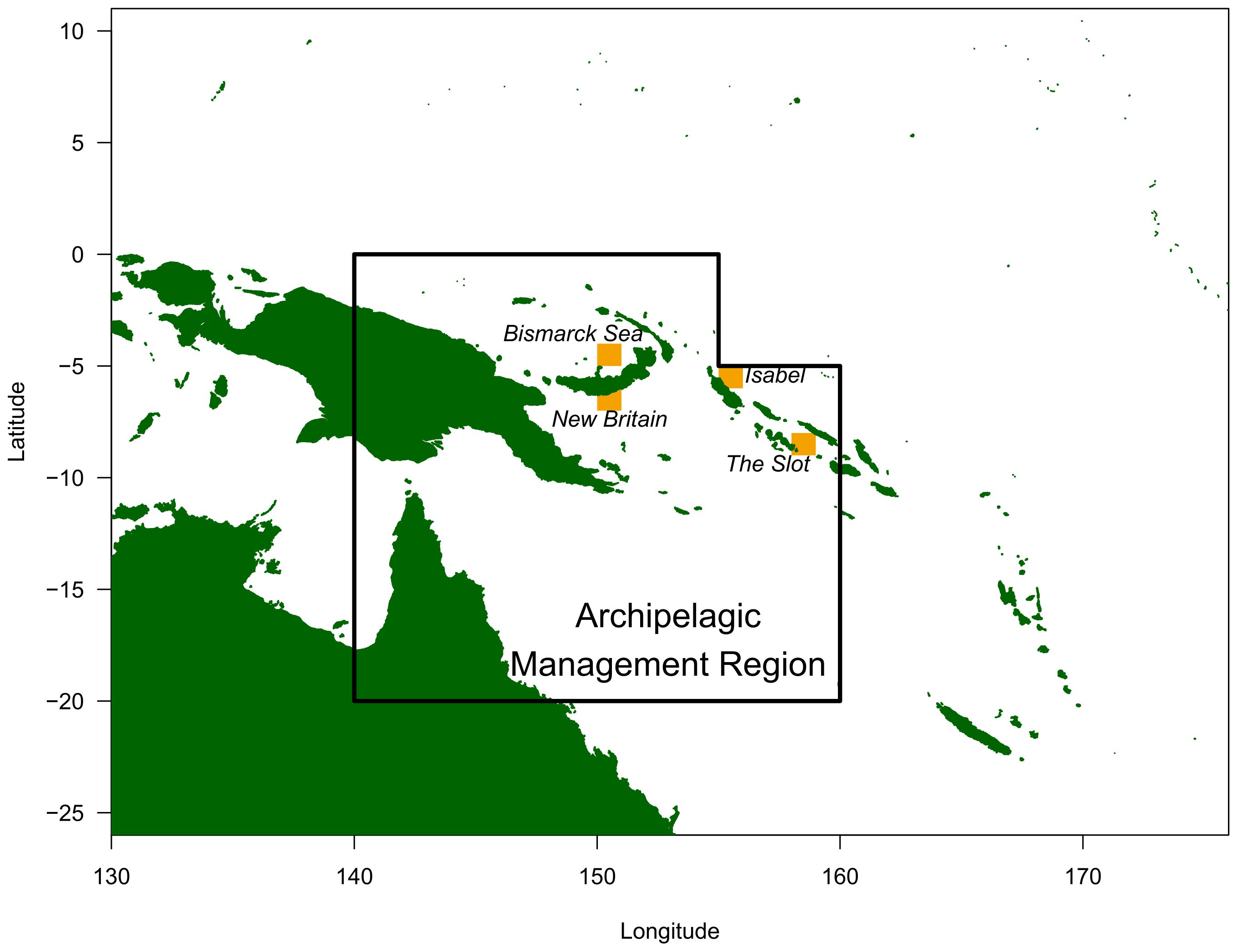
Figure 2. Map of simulated, 1°x1° release locations (yellow) with the archipelagic management region boundary for skipjack tuna marked, as currently assumed within the WCPO convention area.

Table 2

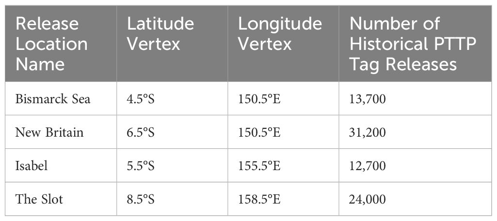
Table 2. Summary of release locations used in simulated CMR experiments, with true numbers of marked individuals released at each as part of the Pacific Tuna Tagging Project.

For the unmarked population, 3 million individuals of the same age were released throughout the Pacific Ocean, with an initial spatial distribution that corresponded to that estimated by the population dynamics model SEAPODYM, and for the same date as each simulated CMR experiment. Differing spatial subsets of these individuals were then used as the reference, unmarked population to which the estimated parameters from the simulated recapture data were compared.

First, we used a subset of unmarked individuals distributed throughout the current management region of interest in which our CMR release locations belong: a large archipelagic region shown in Figure 2. To test the impact of our analytical assumptions, we also examined the impact on bias of changing the spatial extent of the region from which the unmarked population are defined, by using alternate subsets of this population based on the spatial extent of recapture probability of the marked individuals released. This represents a more biologically-based spatial structure for comparison than the fixed management region currently used in stock assessments for this species. In this case, differing proportions of the spatial spread of recaptures after differing periods of time at liberty for each release event were used. These corresponded to the 5%, 25%, 50%, 67% and 95% area of increasing size containing of the greatest recaptures, after one, three and six months at liberty. Only unmarked individuals from within this area, at the time the marked group were released, were used to calculate the realised survival and mortality parameters to which estimated values were compared.

All simulation experiments were run using Ikamoana on Australia’s National Computational Infrastructure (NCI), and divided into parallel model runs of approximately 50,000 particles each. Generation of the environmental fields driving behaviour, and fishing mortality fields driving recapture probability, were pre-calculated and saved per age class-time period combination for efficiency. Each simulation was run on a single core and took ~20 minutes, meaning for each monthly release of marked and corresponding unmarked individuals, the total computation time was approximately 270 hours of computing time.

2.4 Parameter estimation

To estimate the parameters that emerge from our simulated CMR experiments, for which we will examine for bias, we use a common analysis in fisheries science for estimating demographic parameters for animal populations: the Brownie band recovery model (Brownie, 1978b). Using recapture data from multiple release-recapture time periods, the approach estimates average survival S_j and reported recapture probabilities f_j, for each time period j, and assumed shared for each release group cohort.

This model describes the fate of a cohort of N_i marked animals, released at time i. Animals can be recovered in one of several subsequent time periods, or they are never recovered. The number of animals that were released at time i and recovered during time period j is R_ij. The recaptures can be summarised by an upper triangular matrix (Table 3). The sum of each row, r_i, equals the number of individuals in cohort N_i that were recovered over the course of the experiment.

Table 3

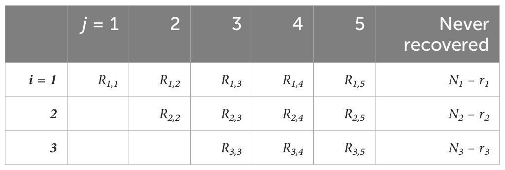
Table 3. Upper triangular matrix describing the numbers of recaptures of fish released at each time period i, over time period j.

Using the IBM approach described above, we populated these upper triangular matrices for each proposed tagging experiment using Equation 4, where

$\begin{array}{ll}{R}_{i,j}={\displaystyle \sum _{n=1}^{N_i}}{p}_n(j) & (5)\end{array}$

for each fish n in R released at time i.

The probability of each entry into the triangular matrix is given by Table 4. We fitted the model using the analytical-numerical estimators described in (Brownie, 1978b; Mann, 1989).

Table 4

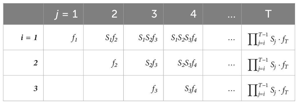
Table 4. Upper triangular matrix describing the assumed probability of marked recapture released at each time period i, over time period j, using Brownie band-recovery mode parameters.

In addition, we also estimate an alternative generalisation of the Brownie model in which, due to lack of instant mixing of marked individuals, each release cohort is assumed to experience a separate probability of recapture $f_i^{*}$ for the period immediately following release.

To examine the parameter bias, we compare the estimates from the Brownie model to the equivalent, realised survival $\overline{s}$ and probability of recapture $\overline{f}$, over time period j, from the simulated marked and unmarked groups. Realised values are the sum of values across all individuals currently at liberty N, weighted by the probability of those individuals having survived prior to time period j. Using Equations 2, 4:

$\begin{array}{ll}{\overline{S}}_j={\displaystyle \sum _{n=1}^N}\frac{s_n(j)}{s_n(j-1)}·{\displaystyle \sum _{n=1}^N}{s}_n(j-1)& (6)\end{array}$

$\begin{array}{ll}{\overline{f}}_j={\displaystyle \sum _{n=1}^N}{p}_n(j)·{\displaystyle \sum _{n=1}^N}{s}_n(j-1)& (7)\end{array}$

3 Results

3.1 Demographics of marked group (Experiments A1 and A2)

To begin, we undertook two simulation experiments to examine parameter estimate bias purely as a function of our Brownie model assumptions, and not due to the assumptions of representativeness of the unmarked population, by comparing estimated against realised parameters from the same group of individuals (Simulations A1 and A2, Table 1). First, we simulated the movement and mortality of 12 monthly releases of marked skipjack tuna with release locations throughout the management region of interest, distributed spatially in proportion to the unmarked population (A1). This represents the hypothetical, ideal CMR experiment for the region, where fish are marked equally throughout the corresponding population, instead of in discrete release locations. Both realised and estimated survival and recapture probability parameters by month for this idealised case are shown in Figure 3A.

Figure 3

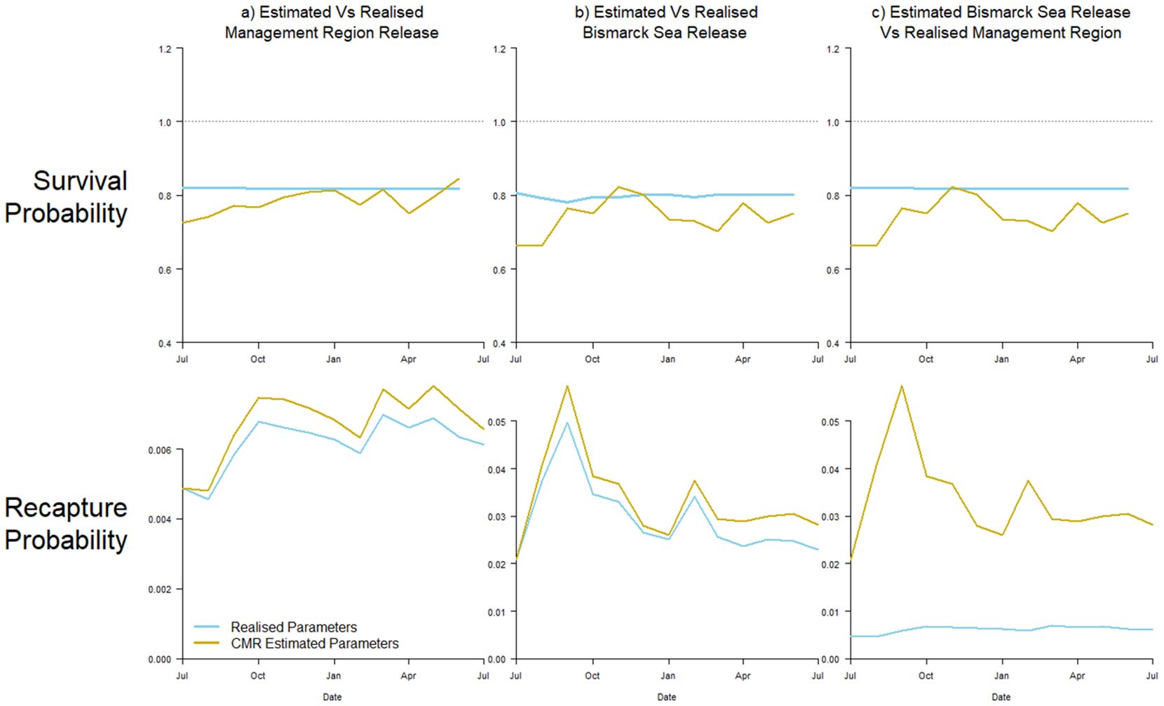
Figure 3. Time-series of estimated (yellow) and realised (blue) parameter values for survival (top) and recapture probability (bottom). Panel (A) shows results from an idealized CMR experiment, with all simulated individuals marked throughout the region. Panel (B) compares estimated and realised parameters of individuals released at the Bismarck Sea location. Panel (C) shows results comparing estimated parameters from marked individuals released at the Bismarck Sea location, against realised parameters from the individuals throughout the region.

Realised parameters show a near-stable survivability S_j through time, which is generally under-estimated using the simple Brownie model. The variability in recapture probability f_j experienced by the group, as a function of changing fishing effort across their area of dispersion, is well tracked but over-estimated. The median, relative bias over time was 4.4% and 9.5% for survival and recapture probability, respectively (Figure 3A).

Undertaking the same exercise, that is, comparing estimated to realised parameters for the same group of individuals, but for individuals released in one of the discrete locations described in Table 1 (The Bismarck Sea, Experiment A2), survival was again generally underestimated, although more variable, and recapture probability overestimated (Figure 3B). Median, relative bias over time was 7.0% and 11.5%, respectively. Realised recapture probability was, however, an order of magnitude greater due to the release of fish in an area of intense fishing, and this was reflected in more variable survival estimates from the simulated recapture data.

3.2 Comparison of marked group to unmarked population (Experiments B1, B2, C1)

To replicate more accurately true CMR experiments, demographic parameters estimated from typical release events were compared against those realised parameters from a regional-scale population of interest (Simulations B1 and B2, Table 1). Figure 3C shows the estimated survival and recapture probability from the Bismarck Sea release scenario against the realised parameters experienced by the unmarked population distributed throughout the management region shown in Figure 2 (B1).

Once again, probability of survival was reasonably well estimated (median, relative bias over time = 9.3%), although fish released in the Bismarck Sea produced a larger, negative bias in these estimates compared to the ‘true’, realised survival of the unmarked population. However, recapture probability estimates were severely overestimated and highly variable, with a median value of 361% greater than that of the unmarked population over time (Figure 3C).

Extending these comparisons, we compared relative bias in estimates from scenarios involving different release sites throughout the historical tagging area, as well as simultaneous releases at all four release locations (Figure 4A, experiment B2). Increasing from a single to multiple release locations decreased bias in survival estimates, from an overall median from all time periods of 9.9% to 6.0% for one to all four locations, respectively. Estimated bias was also most consistent over time for a given combination of locations, with increasing numbers of release locations. For recapture probability estimates, however, while the variability in relative bias over time was reduced with increasing number of release locations, the median bias across all time periods did not improve. Furthermore, the scale of bias was still very large even when individuals were released at all four release locations, with median of 156% (interquartile range 143-234%). While some parameter estimates from individual release scenarios and time periods j were overestimated by nearly 900% (Figure 4A), some individual releases actually outperformed the combined release event scenario when considered over time (e.g. Isabel and New Britain location releases, with time-median errors of 37% and 98%, respectively).

Figure 4

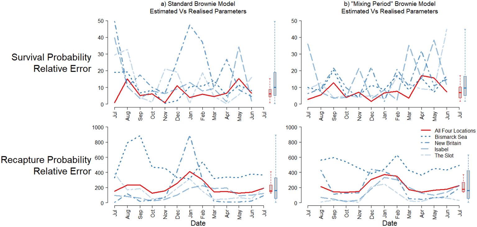
Figure 4. Positive, relative error between estimated and realised parameters for survival (top), and recapture probability (bottom) for different combinations of CMR release location. Left: panel (A) time-series from all each separate release location (blue, dashed and all four (red, solid) release locations. Boxplots show the distribution of all relative parameter errors combined, for the individual release locations (blue) and all four combined (red). Right: panel (B) time-series of the same results, discarding the initial time-period following release for the estimation of population parameters. Note that, when using this approach, recapture probability and survival cannot be estimated during the first and last time periods, respectively.

To examine the effect that large differences in local recovery effort (in this case, fishing pressure) may have on marked individuals immediately post-release, we also fitted Brownie models in which recapture probability during the first period post-release was distinct to that for the other individuals at liberty ($f_i^{*}$, experiment C1, Table 1). Figure 4B shows relative, percentage bias in survival and recapture probability estimates (excluding $f_i^{*}$), for differing release scenarios. Survival estimates had similar bias than for the Brownie model in which $f_i^{*}$ = $f_i$, ranging from overall mean from all time periods of 12.8% to 7.6%, for one to all four locations, respectively. For recapture probability, extreme levels of error were less evident, but time-mean error was again very similar to the simple Brownie model estimates (209% median, interquartile range 104-317%, Figure 4B).

3.3 Comparison of marked groups to local population (Experiments D1 and D2)

We also examined the impact on parameter error of changing the spatial extent of what we consider to be the baseline, unmarked population to which estimates from CMR experiments were compared. We used unmarked individuals from within a spatial boundary around release locations, with that boundary defined by the spatial limit of simulated recapture density of marked individuals, after differing periods of time (experiments D1 and D2, Table 1). As an example, we first examined results using a single release location (D1).

Figure 5 shows this spatial recapture density of the 5%, 50% and 95% areas of greatest recaptures for the New Britain release scenario, after one, three and six months at liberty. When considering the densest 5% area (Figures 5A–C), the great majority of recaptures were focused within the Solomon Sea area and extended east through the archipelago over increasing time from release. When considering the 50% and 95% area of all recaptures (Figures 5D–I), the spatial distribution of recaptures increased to include the wider archipelagic area alongside more oceanic regions to the east. By six months, low recapture numbers were spread out throughout the region, extending as far west as Indonesia and as far east as Fiji by six months of fish being at liberty.

Figure 5

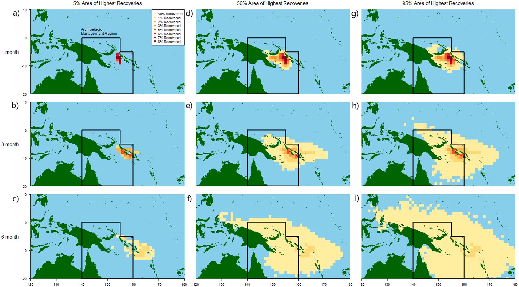
Figure 5. Spatial extent of the 5% (left, A–C), 50% (middle, D–F) and 95% (right, G–I) area of highest numbers of recaptures from marked individuals released at the New Britain location, after one (top, A, D, G), three (middle, B, E, H) and six (bottom, C, F, I) months. Coloured cells show greater (red) or fewer (yellow) recaptures by one degree cell.

Relative error in estimated parameter was calculated using realised parameters from the unmarked population defined by the 95, 67, 50, 25 and 5% area of greatest marked individual recaptures after three months at liberty, respectively (Figure 6). Survival estimates were very similar across all scales of recapture area, with median errors ranging from 13.3% to 12.5% for the areas of 95% and 5% greatest recaptures, respectively (interquartile ranges 8.5-29.2%, 7.1-29.0%). Error in recapture probability estimates was again larger, and highly variable when comparing to the unmarked population over larger areas, from a median of 49% to 51.5%, for 95% and 5% recapture areas, respectively (interquartile ranges 18.0-54.4%, 36.3-74.5%).

Figure 6

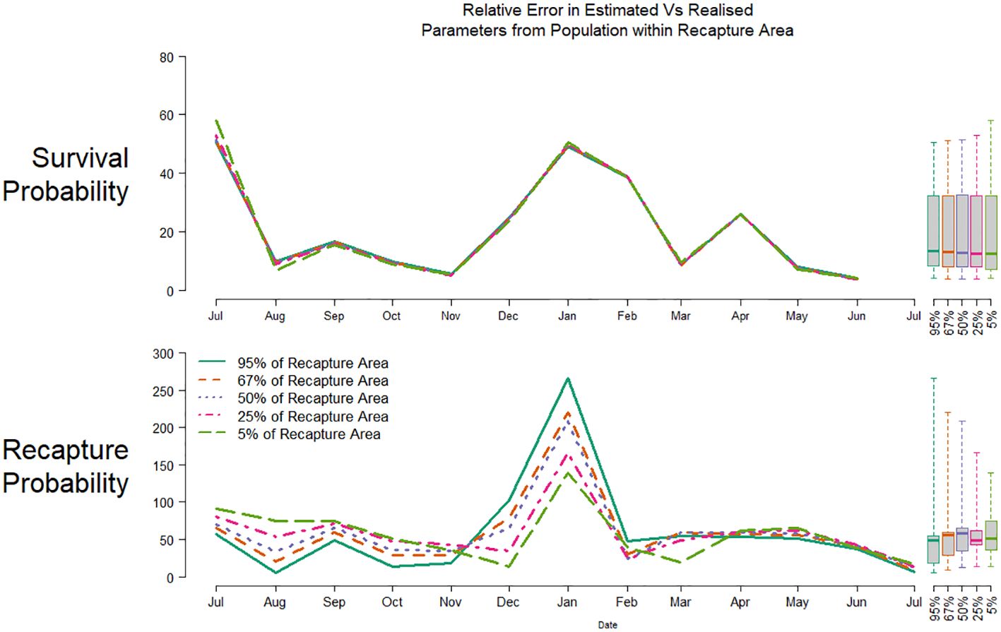
Figure 6. Relative parameter error for survival (top) and recapture probability (bottom) for a CMR experiment releasing individuals in New Britain, comparing estimated against realised parameters from the unmarked population defined by the area covering the 5% (green), 25% (red), 50% (purple), 67% (orange) and 95% (teal) greatest numbers of recaptures. Boxplots show the distributions of all relative parameter errors.

The same exercise was carried out for the combined, four release locations examined previously, this time comparing parameter estimates with the unmarked population from within the same spread of recaptures areas, but after one, three and six months at liberty (experiment D2). The distribution of relative recapture probability errors across all time periods are shown in Figure 7. Survival estimate errors are not shown, as they did not vary from those from Figure 6.

Figure 7

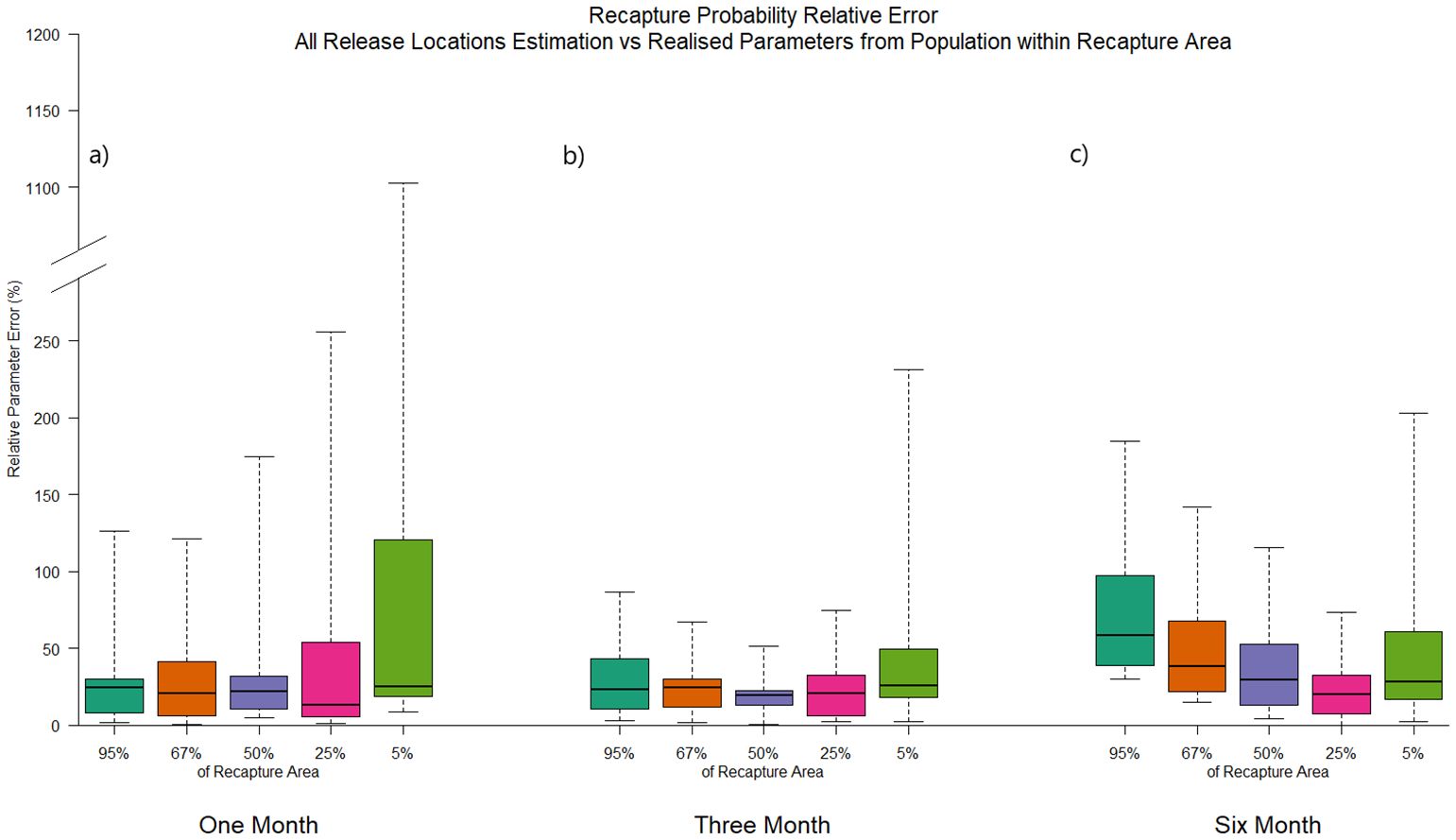
Figure 7. Boxplots of relative parameter error distribution from CMR experiments at all four release locations, comparing estimated parameters against realised from the unmarked population defined by the area covering 5% (green), 25% (red), 50% (purple), 67% (orange) and 95% (teal) greatest numbers of recaptures, after (A) one, (B) three and (C) six months of time-at-liberty.

After only one month at liberty, error in recapture probability estimates had similar variability across all recapture area scales, except for the tightest, 5% recapture area around the four release locations, which was considerably more variable (median error = 25%, interquartile range 19-121%). This can be explained through the relatively short time at liberty of marked individuals resulting in localised and distinct areas of recapture. Comparing recapture probability parameters estimated from releases in an area that experiences high recapture effort, to the realised parameters of an unmarked population made up of individuals from highly localised areas around release locations of varying recapture effort, is more likely to result in larger and more variable bias over time. Despite this, the median, relative parameter error ranged from only 13 to 25% for all recapture areas considered.

Comparing to unmarked fish from the region determined by tag recapture density after three months at liberty, the highest error and variability was again seen for the 5% greatest recapture area, though this was reduced compared to the one month at liberty case. Median error was similar to the latter case for all areas considered, ranging from 20 to 26%.

By six months at liberty, the areas over which recaptures occurred had increased quite considerably, particularly when the extremes of the recapture distribution were included under the 95% greatest recapture density case. This resulted in a clear increase in median error and variability when comparing parameter estimates to the realised recapture probability of unmarked individuals over an increasing area, from 20% to 58% when considering the area covering 25% to 95% of the greatest recoveries, respectively (Figure 7). The exception to this remained the case of comparing estimates to realised parameters from only the area defined by the greatest 5% of tag recaptures around the four tagging release locations, where median, relative error was 27%. Here, once again due to the highly concentrated fishing pressure in the area immediately around the four different release areas even after six months at liberty, there remained high variability between estimated and realised recapture probability.

4 Discussion

In this study, we have demonstrated that using individual-based models incorporating high levels of process heterogeneity can reveal the bias in estimated demographic parameters from capture-mark-recapture experiments. The error present in even the simplest, idealised case we have presented here (that of estimating true, realised parameters of a marked group from recaptures of that same group, Figures 3A, B) demonstrates the limitations of the Brownie model in such a system. The simple fact that the individuals do not all experience the same fishing pressure due to their individual pathways through a spatially varying field of fishing effort leads to estimator bias, particularly for recapture probability parameters. Survival estimate biases were consistent across all our simulations, regardless of experiment design scenario or analytical approach. This is due to our assumed population model, in which natural mortality is a dominant survival process that does not vary spatially, despite being additive to fishing mortality.

While finding bias in parameters estimates for a heterogeneous system, using a model that assumes homogeneity in those processes, is hardly surprising, quantifying the degree of this bias is of value. Despite the clear heterogeneity in our hypothesised system, the relative parameter bias in the idealised cases (of the order of ~10%) may certainly be acceptable for some management decisions. However, examining experimental design and analytical scenarios more typical to those carried out in CMR programmes for this species, we demonstrate a large and likely unacceptable impact on recapture probability estimates, a critically important parameter that is often used to inform levels of fishing mortality in population dynamics models. Our CMR simulations with releases in those locations commonly undertaken in WCPO skipjack tagging experiments typically resulted in recapture probability error in our Brownie model of 100-300% (Figures 3, 4). This is due to marked individuals being released in areas of the management region in which fishing effort is exceptionally high and patchy, often with large recoveries of marked individuals in the months immediately following release. The bias in Brownie model estimates that was already present in the idealised case becomes greatly magnified under these circumstances, in response to the most spatiotemporally heterogeneous processes in our model: environmentally driven movement and fishing effort. While spreading the point of release across varied locations in the region considerably reduced the variability of this error through time, as the spatiotemporal patchiness of fishing effort is more evenly sampled across all individuals, the overall median error in estimates did not change.

Introducing a parameter allowing each release to have a separate recapture probability f* during the initial period following release, is analogous to the ‘mixing period’ commonly applied to CMR data for such species (Peatman et al., 2022). This trades off the discarding of data that cannot be used in the estimation of population-level parameters, as f* is meaningless for the population overall, against decreasing the potential bias caused by lack of mixing from the release location. Our results show that, for skipjack tuna CMR experiments in our example management region, such gains are minimal or non-existent with a mixing period of one month. The spatial scale of the region at which the population being considered exists, alongside the patchy concentration of fishing effort and around the areas used to release individuals, is simply too great for marked individuals to become representative. It is important to note that in stock assessment of this tuna species, mixing periods of much longer than one month are typically explored (Castillo-Jordan et al., 2022), and such time scales could, of course, also be examined using the IBM framework.

The consideration of spatial scale and representativeness in CMR experiments is important, and caution must be taken in applying the results of local-scale experiments to large-scale population models (Zimmermann et al., 2011). The fixed, spatial management region of interest that we have examined in our example is large. Our operating model predicts considerable habitat away from the main areas of fishing, with an associated ‘cryptic’ biomass, which contributes considerably to the high error in recapture probability estimates. In practice, the dimensions of such conservation or management areas may not necessarily depend on the known ecology of a species and the ecosystem, but rather geopolitical contexts, local or state-level jurisdiction, and single- or multi-species conservation policies (Albers et al., 2010). As such, mismatches between the spatial evolution and capture probability of two groups of marked and unmarked animals through time can often occur (Fletcher et al., 2012).

Indeed, the lowest, consistent levels of parameter error we have demonstrated in this study occurred when the assumed spatial coverage was dynamic. When the baseline of the unmarked population to which marked animals were being compared was changed to 25-50% of the area in which recaptures occurred this bias was reduced by around 150% (Figure 7). Rather than hoping to estimate parameters accurately for a population within an arbitrary area, using CMR experiments whose design is more a function of logistics and practicality than the management region, here we use an area defined by the spatial evolution of recaptures themselves to guide our use of these data. In the case of our Pacific skipjack tuna application, this demonstrates the potential benefits of spatial structures that are driven by biologically plausible processes, rather than being fixed or defined by the nature of other data sources (e.g. catch). Similarly, other processes, such as those driving population structure, may influence life history parameter bias within spatially explicit models (Bosley et al., 2022) and can also be examined using our approach.

While adaptive and dynamic spatial management of the marine environment is certainly possible (Maxwell et al., 2015), the difficulty in estimating parameters within data-integrated population dynamics models typically requires fixed spatial structures. Our approach can certainly be used to define or inform the nature of the spatial structure within such models, but more pragmatically it can be used to indicate the spatial or other dimensional limitations on how CMR data can precisely inform models and quantify the potential scale of error.

For example, wildlife managers could choose a degree of bias that is acceptable for decision making, and then use our simulation approach to find the spatial scale at which planned or historical CMR experiments will robustly fulfil these requirements. Once determined, spatial structures can be chosen to make best use of the available data. In the case of fisheries management, models that seek to parameterise growth, connectivity or mortality rates can be constructed to best match the available CMR data. In the case of integrated population dynamics models, where multiple sources of data are used in parameter estimation, CMR data could be used to only inform those parameters of the model that also match this spatial scale, such as in the case of fisheries limiting the influence of recapture data to the estimation of fleet parameters who also operate at the identified spatial scale.

A further benefit of our approach using individual-based modelling is in their flexibility to easily test alternative hypotheses and mechanisms which are not easily estimated in data-driven models. Undertaking such model exploration is important to improve the credibility and appropriateness of existing predictions (Thiele and Grimm, 2015). Wang et al. (2022) undertook such an exercise examining the potential bias in population estimates from CMR experiments on swallowtail butterflies, varying the value of behavioural parameters as well as landscape and sampling effort distributions. They were able to identify recapture effort scenarios that would result in large errors in demographic estimates, as well as those parameters that typical CMR analyses were highly sensitive to for this system. Similarly, Petrovskii et al. (2012) quantified the relationship between insect trap catches and population density, using an IBM with hypotheses on differing diffusion-like behaviours.

In contrast, our example in this study takes the approach of fixing landscape (habitat and fishing mortality fields) and biological (diffusion, taxis and mortality) parameters from existing estimations made on data, and instead focuses on logistical scenarios of experimental design and analytical assumptions to examine bias. However, it would be relatively straightforward to also explore the influence of alternative behavioural scenarios in CMR analyses, and differing assumptions regarding the drivers of behaviour may potentially lead to very different outcomes, which should be explored where valid hypotheses exist for the system. IBMs using individual level attributes or interactions have been used to examine the spatial aggregation of phytoplankton (El Saadi and Bah, 2006), the impacts on catch of fish in response to local aggregation sites (Dagorn et al., 2000; Nooteboom et al., 2023), the expansion of invasive termites (Tonini et al., 2014), and habitat utilisation by jaguars (Watkins et al., 2015). Similarly, our approach can assist with evaluating bias in analyses of existing CMR data to maximise the information derived.

We encourage the use of such hypothesis testing in IBMs for optimising the design and analysis of CMR experiments and related approaches. When the experimental design is spatially limited or local in nature, it is an important tool to characterising spatial extent over which results can provide precise and robust parameter estimates. Similarly, the fields of close-kin mark recapture (Bravington et al., 2016), ecotoxicology (Topping et al., 2009), and telemetry (McClintock, 2021), for species with high levels of behavioural heterogeneity and in patchy landscapes, are likely to benefit from our approach to optimise costly experiments and monitoring programmes.

Data availability statement

The raw data supporting the conclusions of this article will be made available by the authors, without undue reservation.

Author contributions

JS: Conceptualization, Formal analysis, Investigation, Methodology, Software, Visualization, Writing – original draft, Writing – review & editing. JL: Software, Writing – review & editing. IS: Software, Supervision, Validation, Writing – review & editing. RB: Conceptualization, Formal analysis, Methodology, Supervision, Writing – original draft, Writing – review & editing. TP: Conceptualization, Investigation, Methodology, Writing – original draft, Writing – review & editing. MS: Formal analysis, Investigation, Methodology, Writing – review & editing. AS: Conceptualization, Funding acquisition, Investigation, Methodology, Resources, Software, Supervision, Writing – original draft, Writing – review & editing. EV: Conceptualization, Funding acquisition, Investigation, Methodology, Resources, Software, Supervision, Writing – review & editing. SN: Conceptualization, Funding acquisition, Investigation, Methodology, Resources, Supervision, Writing – original draft, Writing – review & editing.

Funding

The author(s) declare financial support was received for the research, authorship, and/or publication of this article. This research was supported by programme funding from the Australian Government Department of Foreign Affairs and Trade. This research was undertaken with the assistance of resources from the National Computational Infrastructure (NCI Australia).

Conflict of interest

The authors declare that the research was conducted in the absence of any commercial or financial relationships that could be construed as a potential conflict of interest.

Publisher’s note

All claims expressed in this article are solely those of the authors and do not necessarily represent those of their affiliated organizations, or those of the publisher, the editors and the reviewers. Any product that may be evaluated in this article, or claim that may be made by its manufacturer, is not guaranteed or endorsed by the publisher.

References

Abadi F., Botha A., Altwegg R. (2013). Revisiting the effect of capture heterogeneity on survival estimates in capture-mark-recapture studies: does it matter? PLoS One 8. doi: 10.1371/journal.pone.0062636

PubMed Abstract | Crossref Full Text | Google Scholar

Albers H. J., Fischer C., Sanchirico J. N. (2010). Invasive species management in a spatially heterogeneous world: Effects of uniform policies. Resour Energy Econ 32, 483–499. doi: 10.1016/j.reseneeco.2010.04.001

Crossref Full Text | Google Scholar

Baranov F. I. (1918). On the question of the biological basis of fisheries.

Google Scholar

Bosley K. M., Schueller A. M., Goethel D. R., Hanselman D. H., Fenske K. H., Berger A. M., et al. (2022). Finding the perfect mismatch: Evaluating misspecification of population structure within spatially explicit integrated population models. Fish Fisheries 23, 294–315. doi: 10.1111/faf.12616

Crossref Full Text | Google Scholar

Bravington M. V., Skaug H. J., Anderson E. C. (2016). Close-kin mark-recapture. Stat. Sci. 31, 259–274. doi: 10.1214/16-STS552

Crossref Full Text | Google Scholar

Brownie C. (1978a). Statistical inference from band recovery data: a handbook (Washington, DC: US Department of the Interior, Fish and Wildlife Service).

Google Scholar

Brownie C. (1978b). Statistical inference from band recovery data: a handbook (Washington, DC: US Department of the Interior, Fish and Wildlife Service).

Google Scholar

Castillo-Jordan C., Teears T., Hampton J., Davies N., Scutt Phillips J., Macdonald J., et al. (2022). Stock assessment of skipjack tuna in the western and central Pacific Ocean: 2022 (Pohnpei, Federated sates of Micronesia: Eighteenth Regular Session of the Scientific Committee of the Western and Central Pacific Fisheries Commission).

Google Scholar

Chadœuf J., Millon A., Bourrioux J., Printemps T., van Hecke B., Lecoustre V., et al. (2018). Modelling unbiased dispersal kernels over continuous space by accounting for spatial heterogeneity in marking and observation efforts. Methods Ecol. Evol. 9, 331–339. doi: 10.1111/mee3.2018.9.issue-2

Crossref Full Text | Google Scholar

Dagorn L., Josse E., Bach P., Bertrand A. (2000). Modeling tuna behaviour near floating objects: from individuals to aggregations. Aquat Living Resour 13, 203–211. doi: 10.1016/S0990-7440(00)01065-2

Crossref Full Text | Google Scholar

Delandmeter P., van Sebille E. (2019). The Parcels v2.0 Lagrangian framework: new field interpolation schemes. Geoscientific Model. Dev. Discussions 12 (8), 3571–3584. doi: 10.5194/gmd-2018-339

Crossref Full Text | Google Scholar

El Saadi N., Bah A. (2006). On phytoplankton aggregation: a view from an IBM approach. C R Biol. 329, 669–678. doi: 10.1016/j.crvi.2006.05.004

PubMed Abstract | Crossref Full Text | Google Scholar

Fletcher D., Lebreton J., Marescot L., Schaub M., Gimenez O., Dawson S., et al. (2012). Bias in estimation of adult survival and asymptotic population growth rate caused by undetected capture heterogeneity. Methods Ecol. Evol. 3, 206–216. doi: 10.1111/j.2041-210X.2011.00137.x

Crossref Full Text | Google Scholar

Grimm V., Railsback S. F. (2005). Individual-based modeling and ecology. BioOne. doi: 10.1515/9781400850624

Crossref Full Text | Google Scholar

Guillemain M., Pradel R., Devineau O., Simon G., Gauthier-Clerc M. (2014). Demographic heterogeneity among individuals can explain the discrepancy between capture-mark-recapture and waterfowl count results. Condor 116, 293–302. doi: 10.1650/CONDOR-13-148.1

Crossref Full Text | Google Scholar

Hampton J., Fournier D. A. (2001). A spatially disaggregated, length-based, age-structured population model of yellowfin tuna (Thunnus albacares) in the western and central Pacific Ocean. Mar. Freshw. Res. 52, 937–963. doi: 10.1071/MF01049

Crossref Full Text | Google Scholar

Hare S. R., Williams P. G., Jordán C. A. C., Hamer P. A., Hampton W. J., Scott R. D., et al. (2021). The Western and Central Pacific Tuna Fishery 2020 Overview and Status of Stocks (Nouméa, New Caledonia: Pacific Community= Communauté du Pacifique).

Google Scholar

Kleiber P., Argue A. W., Kearney R. E. (1987). Assessment of pacific skipjack tuna (Katsuwonus pelamis) resources by estimating standing stock and components of population turnover from tagging data. Can. J. Fisheries Aquat. Sci. 44, 1122–1134. doi: 10.1139/f87-135

Crossref Full Text | Google Scholar

Kolody D., Hoyle S. (2015). Evaluation of tag mixing assumptions in western Pacific Ocean skipjack tuna stock assessment models. Fish Res. 163, 127–140. doi: 10.1016/j.fishres.2014.05.008

Crossref Full Text | Google Scholar

Lauretta M. V., Goethel D. R. (2017). The robustness of Brownie tag return models to complex spatiotemporal dynamics evaluated through simulation analysis. Can. J. Fisheries Aquat. Sci. 74, 1845–1861. doi: 10.1139/cjfas-2016-0291

Crossref Full Text | Google Scholar

Leroy B., Nicol S., Lewis A., Hampton J., Kolody D., Caillot S., et al. (2013). Lessons learned from implementing three, large-scale tuna tagging programmes in the western and central Pacific Ocean. Fish Res. 163, 23–33. doi: 10.1016/j.fishres.2013.09.001

Crossref Full Text | Google Scholar

Lindberg M., Rexstad E. (2001). “Capture–recapture sampling designs,” in Encyclopedia of Environmetrics. doi: 10.1002/9780470057339.vac003

Crossref Full Text | Google Scholar

Mann R. (1989). “Design and analysis methods for fish survival experiments based on release-capture,” in American Fisheries Society Monograph 5 (1987), vol. 4 . Eds. Burnham K. P., Anderson D. R., White G. C., Brownie C., Pollock K. H. (American Fisheries Society, Maryland, U.S.A), 437, ISBN: ISBN (hard) 0-913235-41-5. Regulated Rivers: Research & Management. doi: 10.1002/rrr.3450040111

Crossref Full Text | Google Scholar

Mathur R. (2007). An evaluation of the Brownie tag-recapture model using simulation-estimation procedures, with application to British Columbia sablefish (Anoplopoma fimbria) (Toronto, Canada: Simon Fraser University).

Google Scholar

Maxwell S. M., Hazen E. L., Lewison R. L., Dunn D. C., Bailey H., Bograd S. J., et al. (2015). Dynamic ocean management: Defining and conceptualizing real-time management of the ocean. Mar. Policy 58, 42–50. doi: 10.1016/j.marpol.2015.03.014

Crossref Full Text | Google Scholar

McClintock B. T. (2021). Worth the effort? A practical examination of random effects in hidden Markov models for animal telemetry data. Methods Ecol. Evol. 12, 1475–1497. doi: 10.1111/2041-210X.13619

Crossref Full Text | Google Scholar

Meli M., Auclerc A., Palmqvist A., Forbes V. E., Grimm V. (2013). Population-level consequences of spatially heterogeneous exposure to heavy metals in soil: An individual-based model of springtails. Ecol. Modell 250, 338–351. doi: 10.1016/j.ecolmodel.2012.11.010

Crossref Full Text | Google Scholar

Moqanaki E. M., Milleret C., Tourani M., Dupont P., Bischof R. (2021). Consequences of ignoring variable and spatially autocorrelated detection probability in spatial capture-recapture. Landsc Ecol. 36, 2879–2895. doi: 10.1007/s10980-021-01283-x

Crossref Full Text | Google Scholar

Nooteboom P. D., Scutt Phillips J., Senina I., van Sebille E., Nicol S. (2023). Individual-based model simulations indicate a non-linear catch equation of drifting Fish Aggregating Device-associated tuna. ICES J. Mar. Sci. 80 (6), 1746–1757. doi: 10.1093/icesjms/fsad105

Crossref Full Text | Google Scholar

Peatman T., Vincent M. T., Scutt Phillips J., Nicol S. (2022). Times are changing, but has natural mortality? Estimation of mortality rates for tropical tunas in the western and central Pacific Ocean. Fish Res. 256. doi: 10.1016/j.fishres.2022.106463

Crossref Full Text | Google Scholar

Pépino M., Rodríguez M. A., Magnan P. (2012). Fish dispersal in fragmented landscapes: A modeling framework for quantifying the permeability of structural barriers. Ecol. Appl. 22, 1435–1445. doi: 10.1890/11-1866.1

PubMed Abstract | Crossref Full Text | Google Scholar

Pépino M., Rodríguez M. A., Magnan P. (2016). Assessing the detectability of road crossing effects in streams: mark–recapture sampling designs under complex fish movement behaviours. J. Appl. Ecol. 53, 1831–1841. doi: 10.1111/1365-2664.12725

Crossref Full Text | Google Scholar

Petrovskii S., Bearup D., Ahmed D. A., Blackshaw R. (2012). Estimating insect population density from trap counts. Ecol. Complexity 10, 69–82. doi: 10.1016/j.ecocom.2011.10.002

Crossref Full Text | Google Scholar

Pine W., Pollock K., Hightower J., Kwak T., Rice J. (2003). A review of tagging methods for estimating fish population size and components of mortality. Fisheries (Bethesda) 28, 10–23. doi: 10.1577/1548-8446(2003)28[10:AROTMF]2.0.CO;2

Crossref Full Text | Google Scholar

Pledger S. (2005). The performance of mixture models in heterogeneous closed population capture-recapture. Biometrics 61, 351–364. doi: 10.1111/j.1541-020X.2005.00411_1.x

PubMed Abstract | Crossref Full Text | Google Scholar

Pledger S., Efford M. (1998). Correction of bias due to heterogeneous capture probability in capture- recapture studies of open populations. Biometrics 54, 888–898. doi: 10.2307/2533843

Crossref Full Text | Google Scholar

Pollock K. H., Jiang H., Hightower J. E. (2004). Combining telemetry and fisheries tagging models to estimate fishing and natural mortality rates. Trans. Am. Fish Soc. 133, 639–648. doi: 10.1577/T03-029.1

Crossref Full Text | Google Scholar

Rees S. G., Goodenough A. E., Hart A. G., Stafford R. (2011). Testing the effectiveness of capture mark recapture population estimation techniques using a computer simulation with known population size. Ecol. Modell 222, 3291–3294. doi: 10.1016/j.ecolmodel.2011.05.030

Crossref Full Text | Google Scholar

Sandercock B. K. (2006). “Handbook of capture-recapture analysis,” in Biometrics, vol. 62. Eds. Amstrup S. C., Mcdonald T. L., Manly B. F. J.. (Princeton, New Jersey: Princeton University Press). doi: 10.1111/j.1541-0420.2006.00596_10.x

Crossref Full Text | Google Scholar

Schaub M., Royle J. A. (2014). Estimating true instead of apparent survival using spatial Cormack–Jolly–Seber models. Methods Ecol. Evol. 5, 1316–1326. doi: 10.1111/mee3.2014.5.issue-12

Crossref Full Text | Google Scholar

Scutt Phillips J., Sen Gupta A., Senina I., van Sebille E., Lange M., Lehodey P., et al. (2018). An individual-based model of skipjack tuna (Katsuwonus pelamis) movement in the tropical Pacific ocean. Prog. Oceanogr 164, 63–74. doi: 10.1016/j.pocean.2018.04.007

Crossref Full Text | Google Scholar

Senina I., Lehodey P., Sibert J., Hampton J. (2020). Integrating tagging and fisheries data into a spatial population dynamics model to improve its predictive skills. Can. J. Fisheries Aquat. Sci. 77, 576–593. doi: 10.1139/cjfas-2018-0470

Crossref Full Text | Google Scholar

Sippel T., Paige Eveson J., Galuardi B., Lam C., Hoyle S., Maunder M., et al. (2014). Using movement data from electronic tags in fisheries stock assessment: A review of models, technology and experimental design. Fish Res. 163, 152–160. doi: 10.1016/j.fishres.2014.04.006

Crossref Full Text | Google Scholar

Thiele J. C., Grimm V. (2015). Replicating and breaking models: good for you and good for ecology. Oikos 124, 691–696. doi: 10.1111/oik.2015.v124.i6

Crossref Full Text | Google Scholar

Tonini F., Hochmair H. H., Scheffrahn R. H., DeAngelis D. L. (2014). Stochastic spread models: A comparison between an individual-based and a lattice-based model for assessing the expansion of invasive termites over a landscape. Ecol. Inform 24, 222–230. doi: 10.1016/j.ecoinf.2014.09.011

Crossref Full Text | Google Scholar

Topping C. J., Dalkvist T., Forbes V. E., Grimm V., Sibly R. M. (2009). The potential for the use of agent-based models in ecotoxicology. Ecotoxicology Modeling, 205–235. doi: 10.1007/978-1-4419-0197-2_8

Crossref Full Text | Google Scholar

Tourani M. (2022). A review of spatial capture–recapture: Ecological insights, limitations, and prospects. Ecol. Evol. 12. doi: 10.1002/ece3.8468

PubMed Abstract | Crossref Full Text | Google Scholar

Vangestel C., Mergeay J., Dawson D. A., Vandomme V., Lens L. (2011). Spatial heterogeneity in genetic relatedness among house sparrows along an urban–rural gradient as revealed by individual-based analysis. Mol. Ecol. 20, 4643–4653. doi: 10.1111/j.1365-294X.2011.05316.x

PubMed Abstract | Crossref Full Text | Google Scholar

Vincent M. T., Pilling G. M. (2023). Assumptions influencing the estimation of natural mortality in a tag-integrated statistical model for western and central Pacific Ocean skipjack. Fish Res. 261. doi: 10.1016/j.fishres.2023.106612

Crossref Full Text | Google Scholar

Wang Z., Li Y., Jain A., Pierce N. E. (2022). Agent-based models reveal limits of mark–release–recapture estimates for the rare butterfly, Bhutanitis thaidina (Lepidoptera: Papilionidae). Insect Sci. 29, 550–566. doi: 10.1111/1744-7917.12949

PubMed Abstract | Crossref Full Text | Google Scholar

Wang Y.-G., Thomas M. R., Somers I. F. (1995). A maximum likelihood approach for estimating growth from tag–recapture data. Can. J. Fisheries Aquat. Sci. 52, 252–259. doi: 10.1139/f95-025

Crossref Full Text | Google Scholar

Watkins A., Noble J., Foster R. J., Harmsen B. J., Doncaster C. P. (2015). A spatially explicit agent-based model of the interactions between jaguar populations and their habitats. Ecol. Modell 306, 268–277. doi: 10.1016/j.ecolmodel.2014.10.038

Crossref Full Text | Google Scholar

Zimmermann K., Fric Z., Jiskra P., Kopeckova M., Vlasanek P., Zapletal M., et al. (2011). Mark-recapture on large spatial scale reveals long distance dispersal in the marsh fritillary, Euphydryas aurinia. Ecol. Entomol. 36, 499–510. doi: 10.1111/j.1365-2311.2011.01293.x

Crossref Full Text | Google Scholar