Evaluation of the effects of Argo data quality control on global ocean data assimilation systems

A series of observing system experiments (OSEs) were conducted in order to evaluate the effects of Argo data quality control (QC), by using the three global ocean data assimilation systems. During the experimental period between 2015 and 2020, some Argo floats are affected by the abrupt salinity drifts, which caused spurious increasing trend of the global mean salinity in the reanalyses using the observations with only real-time QC applied. The spurious trend is mitigated by applying the gray list provided by the Argo Global Data Assembly Centres (GDAC), and further reduced by assimilating the delayed-mode Argo data of the Argo GDAC instead of the real-time Argo data. These impacts of the Argo QC are generally consistent among the three ocean data assimilation systems. Further investigations in the JMA’s system show that errors in the analyzed salinity with respect to the delayed-mode Argo data are smaller in the OSE with more rigorous QC, and the spatiotemporal variations in the sea-surface dynamic height are reproduced better. Additionally, QC impacts on the analyzed temperatures are shown not to directly reflect the difference in temperature observations among OSEs, and may be affected by difference in the salinity observations among OSEs through the cross-covariance relationship in the data-assimilation systems.

1 Introduction

An Argo float drifts with the ocean currents and autonomously observes the vertical profile of water temperature, salinity, and pressure from a depth of 2,000 meters to the sea surface once every 10 days, transmitting the results via satellite. Currently, approximately 4,000 Argo floats are deployed in the global oceans, and they constitute the largest part of the in-situ ocean observing system. They have provided over two-million vertical profiles of temperature and salinity in the last 20 years since the global Argo program started (Argo, 2022). This large dataset is used for ocean and climate monitoring and initializations of ocean and coupled atmosphere-ocean predictions, including subseasonal-to-seasonal (S2S) forecasts, through ocean data assimilation. However, it is known that about 15 percent of Argo floats deployed after 2015 have experienced abrupt large salinity drifts, which are believed to be due to a conductivity sensor failure (Wong et al., 2020). Use of the data without adjustment in ocean data assimilation generally leads to spurious increasing salinity trends, which will be demonstrated in this study. The manufacturer of the sensor has changed its production line in 2018 to solve this problem (Wong et al., 2023).

Argo profiles are first reported to the Argo Data Assembly Centers (DACs). Once the DACs receive the profiles, they perform a simplified quality control (QC) called real-time QC, and then release them through the Argo Global Data Assembly Centres (GDAC) and the Global Telecommunication System (GTS) for operational use a few hours to a few days after the observation time. Subsequently, the DACs apply more rigorous QC, or delayed-mode QC, to the profiles, and release them through the GDAC for research purposes months to years later. In addition, the GDAC provides a gray list of floats reporting observation data of doubtful accuracy. The floats suffering from the abrupt salinity drifts (ASDs) are listed on the gray list and flagged as bad data by the delayed-mode QC. After ASDs were detected, the real-time QC also excludes the floats with ASDs. In the delayed-mode QC, data affected by smaller salinity drifts or reduced accuracy due to other reasons are also identified and either adjusted or flagged as unadjustable (bad) data (Wong et al., 2023).

Ocean data assimilation systems generally have their own QC procedure, by which most profiles that have suffered ASD are expected to be withheld from assimilation. However, it remains possible that the QC procedure misses to identify a small number of profiles affected by ASD and more profiles with smaller salinity drift. In this study, we, therefore, investigate the impact of those erroneous profiles on the outcome of ocean data assimilation experiments. Both the real-time and delayed-mode QCs by the Argo DACs, along with the application of the gray list, can exclude or modify the erroneous profiles and are expected to mitigate the loss of accuracy caused by those profiles. The impact of these corrections is also evaluated in this study.

A series of observing system experiments (OSEs) are conducted with Argo data from different QC stages: data without QC, data with real-time QC, data with the gray list applied, and data after the delayed-mode QC. Here, we use the global ocean data assimilation system for seasonal forecasting operations in the Japan Meteorological Agency (JMA) for the OSEs, and the results are compared with results of similar OSEs conducted by the European Centre for Medium-Range Weather Forecasts (ECMWF) and the Bjerknes Centre for Climate Research (BCCR).

The remainder of this paper is organized as follows, Section 2 describes the configuration of the OSEs, the results are presented in Section 3, followed by the summary and discussions in Section 4.

2 Models and the OSEs

2.1 OSE setting conducted in JMA

This study mainly analyzes the results from the OSEs using JMA’s operational global ocean data assimilation system MOVE/MRI.COM-G3 (Fujii et al., 2023), which is currently used to initialize the ocean component of the JMA’s coupled atmosphere-ocean prediction system Version 3 (CPS3; Hirahara et al., 2023). CPS3 is used for the seasonal forecasting operations, and provides sea surface temperature (SST) fields for monthly atmospheric forecasting operations. The ocean data assimilation system MOVE/MRI.COM-G3 consists of a low-resolution analysis model MOVE-G3A and a high-resolution forecast model MOVE-G3F; MOVE-G3A is used exclusively here. The physical model of MOVE-G3A consists of Meteorological Research Institute Community Ocean Model Version 4 (MRI.COM Ver. 4; Tsujino et al., 2017). It adopts a tripolar grid (Murray, 1996) over the global domain with a zonal resolution of 1° and the meridional resolution of 0.3-0.5° with refinement near the equator. It adopts the rescaled height coordinate system (so-called z^*-coordinate; Adcroft and Campin, 2004), and has 60 vertical levels and a bottom boundary layer (Nakano and Suginohara, 2002). A five-category sea-ice model, based on the thermodynamic formulation of Mellor and Kantha (1989) and the elastic-viscous-plastic dynamic formulation of Hunke and Lipscomb (2006) with a ridging and rheology scheme, is also incorporated. Ocean observation data including in-situ temperature and salinity profiles, SSTs, and sea surface heights (SSHs) are assimilated into the model through a four-dimensional variational (4DVAR) scheme (Usui et al., 2015) with a five-day observation window. Sea ice concentration data are also assimilated with a separated three-dimensional variational (3DVAR) scheme (Toyoda et al., 2016).

In this study, we conduct the following four OSEs in which Argo data from different QC stages are assimilated. The first OSE is the control experiment (CNTL) which assimilates temperature and salinity observation data distributed through GTS. The observation data include the Argo data to which the real-time QC is applied and in situ observation data from other observational platforms. Here, data with flags other than 0 (no QC performed), 1 (good data), and 5 (value changed) are excluded, as well as data reported more than five days after being observed. This OSE is thus expected to produce results similar to the operational analysis. The second OSE named ‘GLST’ uses the same temperature and salinity observation data as CNTL except that the Argo profiles in the gray list are excluded. The third OSE named ‘DELAY’ uses the same temperature and salinity data as GLST except that the Argo data with the real-time QC applied are replaced by the delayed-mode data when the delayed-mode data are available from the snapshot of the Argo GDAC in Oct. 2021. The fourth OSE named ‘NOQC’ uses the same temperature and salinity data as CNTL except that the Argo data with the real-time QC applied are replaced by raw observed values of Argo data in the Argo GDAC snapshot in Oct. 2021 and the flags for the Argo data are ignored. In addition, the following two OSEs, in which the 3DVAR option of MOVE-G3A is used instead of the 4DVAR to save computational resources, are conducted to examine the effect of the reduction in the amount of delayed-mode data after 2019 contained in the Oct. 2021 snapshot. One is ‘DELAY3DV’ which assimilate the same temperature and salinity observation data as DELAY. The other is ‘DELAY3DVN’ which is the same as ‘DELAY3DV’ but the delayed-mode Argo data are collected from the Argo GDAC snapshot in Mar. 2023 instead of the snapshot in Oct. 2021. In addition, the ocean model free run (‘FREE’) is also used for comparison with the assimilation experiments.

The numbers of Argo profiles used in the JMA’s OSEs are shown in Figure 1. While the total number of profiles has remained largely unchanged, the number of profiles being gray-listed has gradually increased. In contrast, the number of profiles corrected by the delayed-mode QC (202110) has been decreasing after 2019, but a significant number of profiles have been added in the newer version (202303), which was acquired after all the OSEs but DELAY3DVN were completed. This may reflect the fact that delayed-mode QC requires a certain time to be complete.

Figure 1

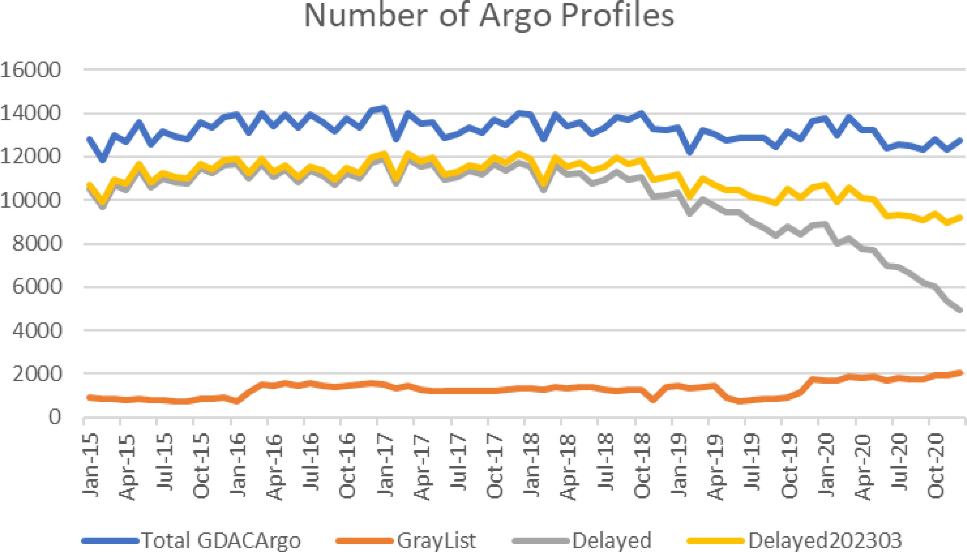
Figure 1. Monthly number of the all GDAC Argo profiles (blue), profiles listed as gray (orange), profiles subjected to delayed-mode QC (gray), a newer version of the delayed-mode profiles (yellow).

All OSEs except FREE also assimilate the reprocessed along-track sea level anomaly data from Copernicus Marine and Environment Monitoring Service (CMEMS, 2023a) and SST and sea ice concentration data from Merged satellite and in situ Global Daily Sea Surface Temperature (MGDSST), produced by JMA (Kurihara et al., 2006). All OSEs are conducted for the years from 2015 to 2020. The initial conditions at the beginning of 2015 for all OSEs and FREE run are the same, and come from the ocean reanalysis (‘4DVAR’ run) conducted by Fujii et al. (2023). Atmospheric forcing at the ocean surface comes from the JRA-3Q (Kosaka et al., 2024) atmospheric reanalysis.

In all OSEs, the following QC procedures are applied to temperature and salinity profiles to be assimilated into G3A. First, the profiles are interpolated to the model standard levels, and observations of temperature below -1.8°C or above 50°C and salinity below 0 psu or above 50 psu are discarded. Next, the temperature profiles are approximately converted to the potential temperature profiles using temperature and depth values. Then, the potential temperatures and salinities that deviate from the background values by more than four times the standard difference between background and the observed values are discarded as bad data. Each set of temperature and salinity profiles with more than five bad data is also discarded. Furthermore, the variational QC scheme proposed by Fujii et al. (2005) has also been incorporated in G3A, in which the weight is reduced (nullified) for the temperature and salinity observations that deviate from the analysis by more than 1.5 (3) times the prescribed standard difference between background and observed values.

2.2 OSE setting conducted in ECMWF

Only the equivalent to the CNTL and DELAY OSEs have been conducted using the ECMWF OCEAN5 system (Zuo et al., 2019). OCEAN5 is based on the NEMO3.4 framework (Madec, 2008) at a 1/4° horizontal resolution and 75 vertical levels with level spacing increasing from 1 m at the surface to 200 m in the deep ocean. The data assimilation is conducted using the NEMOVAR system (Weaver et al., 2005; Mogensen et al., 2012) in its 3D-Var FGAT configuration and 5-day assimilation window. Observation used in data assimilation includes temperature and salinity profiles, sea-ice concentration from near-real-time OSTIA dataset (Donlon et al., 2012) and altimeter derived along-track sea-level anomalies (SLA) data (Pujol et al., 2016). The sea surface temperature (SST) from OSTIA is also used to constrain ocean upper temperature through a simple nudging scheme. The atmospheric forcing comes from the ECMWF NWP operations. In CNTL, the assimilated in-situ temperature and salinity profiles come from the GTS with real-time QC. In DELAY, the assimilated profiles come from the reprocessed EN4 dataset (Good et al., 2013).

2.3 OSE setting conducted in BCCR

NorCPM1 (Bethke et al., 2021) is used to conduct OSEs in this study. NorCPM1 is developed with BCCR and combines the Norwegian Earth System Model (Bentsen et al., 2013) with an ensemble Kalman filter (Evensen, 2003). It has been developed for climate reanalysis and has been employed for the Decadal Climate Prediction Project (DCPP) as part of the sixth Coupled Model Intercomparison Project (CMIP6) (Bethke et al., 2021). The atmosphere and land components have a horizontal resolution of 1.9° of latitude and 2.5° of longitude. The ocean and sea ice components have a horizontal resolution of approximately 1°. The ocean component comprises a stack of 51 isopycnic layers, with a bulk mixed layer representation on top consisting of two layers with time-evolving thicknesses and densities. NorCPM1 comprises 30 ensemble members.

The data assimilation implementation of NorCPM1 has been documented in Bethke et al. (2021). In this study, NorCPM1 conducts four OSEs as follows:

● CNTL: NorCPM1 assimilates temperature and salinity observation data with real-time QC from the Argo GDAC (Oct. 2021). Data with flags other than 0 (no QC performed), 1 (good data), and 5 (value changed) are excluded.

● GLST: similar to CNTL, but the Argo profiles in the gray list are excluded.

● DELAY: similar to GLST, but the Argo data with the real-time QC are replaced by the delayed-mode data when the delayed-mode data are available.

● NOQC: similar to CNTL, but the QC flags are ignored.

In all experiments, NorCPM1 assimilates SST data from the OISSTV2 dataset in addition to profile data assimilation. The observations of temperature below -2.5°C or above 35°C and salinity below 1 psu or above 50 psu are discarded, which is applied to all experiments.

3 Results

3.1 Impacts of the QCs on the salinity field

First, we examine the time series of the global mean salinity from the sea surface to 2000 m depth (the depth sampled by the Argo floats) over the 2015-2020 period for each OSE (Figure 2). In the MOVE-G3A results, CNTL indicates an overall increasing trend, especially in the first half of the six-year period. GLST shows a slightly smaller tendency to increase than CNTL, and in DELAY, the increasing salinity trend is even smaller. On the other hand, NOQC shows a larger increasing salinity trend than CNTL, especially in the latter half of the experimental period. The OCEAN5 results are consistent with those of MOVE-G3A in that both OSEs also show an increasing salinity trend and the trend in DELAY is smaller than in CNTL.

Figure 2

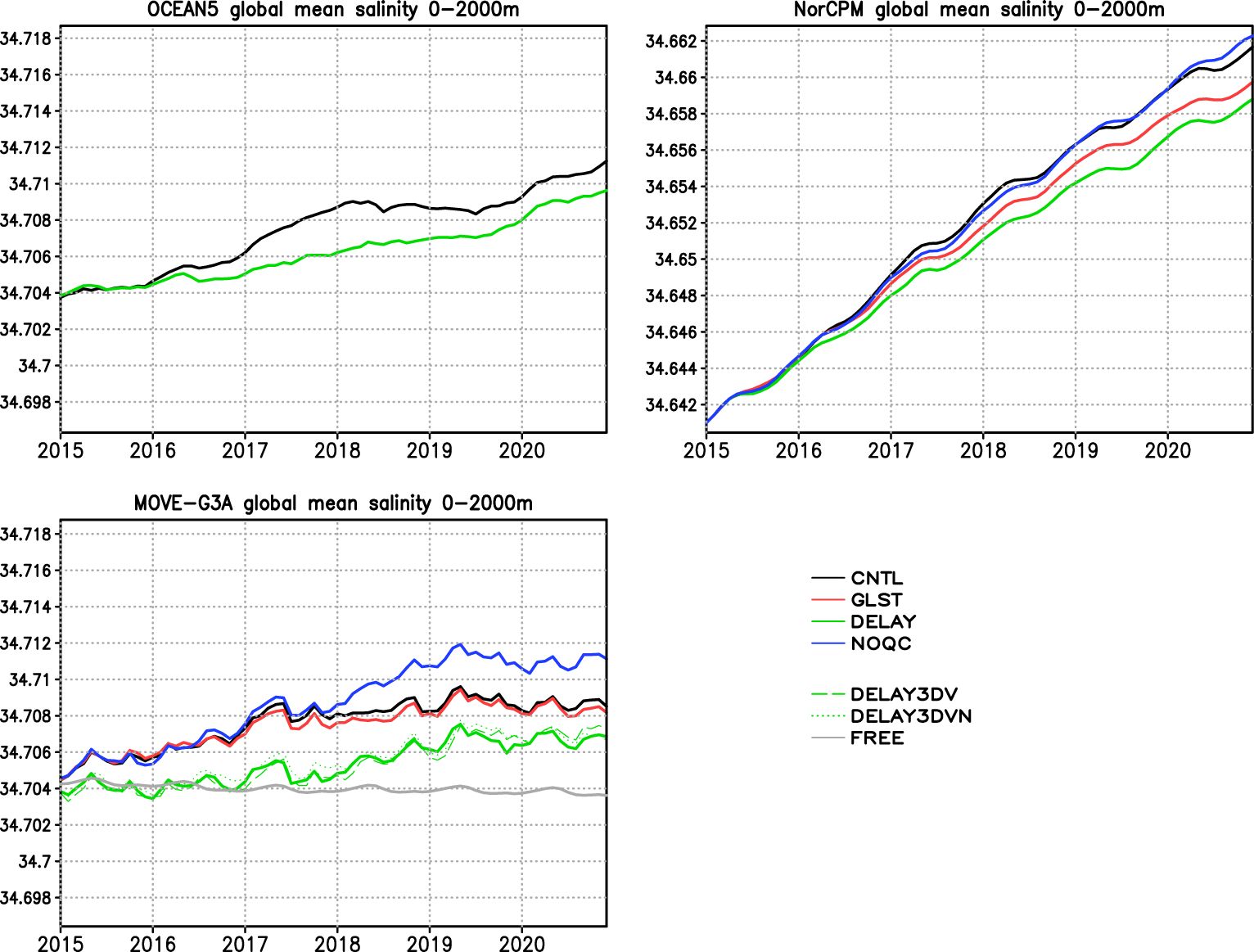
Figure 2. Time-series of the global mean salinity in the upper 2000m. Upper left panel: OCEAN5; upper right panel: NERSC; lower panel: MOVE-G3A. Black line indicates CNTL; red line GLST; green line DELAY; blue line NOQC. For MOVE-G3A, DELAY3DV (green dashed line) and DELAY3DVN (green dotted line), FREE (gray line) are also shown.

The NorCPM system is originally an anomaly-field assimilation system, which assimilates observation anomalies. The OSEs, however, switched to the full-field assimilation, resulting in an overall increasing salinity drift much larger than the salinity trends seen in the OSEs with the other systems (note that the values on the vertical axis are out of alignment with the other panels, and there are lower salinity values in the NorCPM’s OSEs than the other systems; the scales of the vertical axes are adjusted so that the magnitude of change can be compared among the systems). While most of this drift is unrelated to the observation data, the impacts of assimilating different data, which can be seen through comparison between OSEs, are consistent with other systems, as they are NOQC, CNTL, GLST, and DELAY, in order of magnitudes of the increasing salinity trend.

It should be noted that the global mean salinity in FREE of MOVE-G3A (OGCM free run without data assimilation) remains almost constant over the experimental period, which is because, in the ocean model formulation, there is no salinity input and the freshwater inflow in the global ocean (here, sea ice is regarded as part of the global ocean) is adjusted to zero. Salt exchange between the layers above and below 2000 m depth can change the global mean salinity, but the exchange is too small to cause no-negligible change in the model. The stable global mean salinity in FREE indicates that the increase in salinity in the OSEs is due to data assimilation.

It is valuable to examine the effect of the data assimilation system as well as the reduction in the amount of delayed-mode data toward the end of the experimental period. In order to examine that effect, we compare the time-series of the global mean salinity between DELAY and the two 3DVAR OSEs that use MOVE-G3A (DELAY3DV and DELAY3DVN). There are only small differences between DELAY and DELAY3DV, meaning that the difference in the data assimilation schemes do not have a significant impact on the global mean salinity. Then, the small difference between DELAY3DV and DELAY3DVN indicates that the reduction of the delayed-mode data toward the end of the experimental period has only a small impact. It can, thus, be assumed that the decrease in the difference between CNTL and DELAY at the end of the experimental period is not due to the reduction in the amount of delayed-mode data.

To illustrate the spatial pattern of the salinity trend, we show the maps of vertical mean salinity differences between the years 2015-16 and 2019-2020 for the DELAY with the three assimilation systems (Figure 3). There are only small differences in the salinity trend patterns among OSEs using MOVE-G3A that are not visually apparent, as shown by comparing results from NOQC and DELAY from MOVE-G3A in Figure 3. The patterns are also consistent between OCEAN5 and MOVE-G3A, in that the relatively large increasing trends are found in the northwestern part of the North Pacific and the North Atlantic and the western part of the tropical Pacific, near the Californian coast and in the subtropical Indian Ocean. The significant large increasing trend is also found in those regions for the DELAY of NorCPM although it has much larger increasing trends in many regions than the other two systems, which is considered due to the experimental setting mentioned above. The DELAY OSEs of MOVE-G3A and OCEAN5 also have common significant decreasing trends in the northeastern part of the North Pacific and the western and central part of the North Pacific subtropical band, and smaller decreasing trends are found in these regions in the OSEs of NorCPM. The horizontal patterns of the increasing and decreasing trends are consistently represented by the three systems.

Figure 3

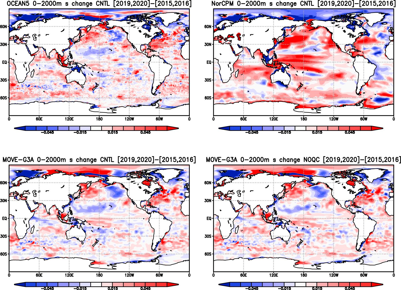
Figure 3. Horizontal distribution of difference in salinity averaged for upper 2000m between 2019-20 and 2015-16 in the DELAY OSE: upper left: OCEAN5, upper right: NERSC, lower left: MOVE-G3A. The result from NOQC OSE with MOVE-G3A is shown for comparison in the lower right panel.

QC impacts on mean salinities in 2019-2020 represented by differences between the CNTL and DELAY are compared among the three systems in Figure 4. Positive values in many areas of the ocean are common across the systems, reflecting that the delayed mode QC corrects for smaller salinity drift across the global ocean in all of the systems. It should be noted that, however, the horizontal patterns are not as consistent among the three systems as those of salinity trends shown above (Figure 3). This may be because the observation data input to each OSE are not necessarily the same among the systems (e.g. satellite altimetry data are not assimilated in NorCPM), and/or because of differences in data assimilation schemes (e.g. de-correlation length-scales used in OCEAN5 covariance formulation is clearly shorter than those used by the NorCPM system) In addition, different settings about the relative importance of various observing systems are also considered to potentially affect the Argo observation impacts on assimilation results.

Figure 4

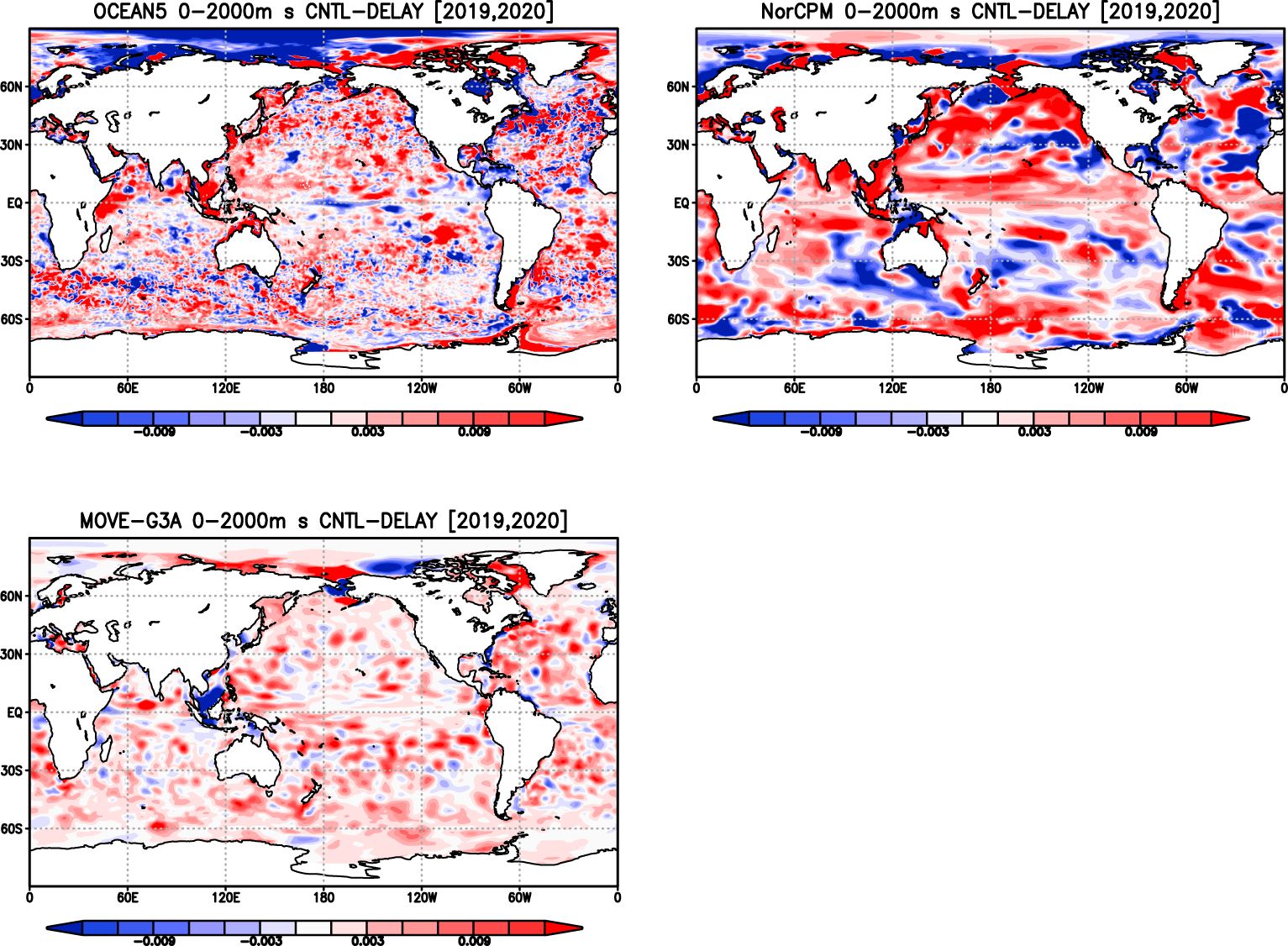
Figure 4. QC impacts (CNTL-DELAY) on mean salinity for 0-2000m in 2019-2020 for OCEAN5 (top-left), NorCPM (top-right), and MOVE-G3A (bottom-left).

In the following, the impact of QC is shown as the difference between the NOQC and the other OSEs, to examine how the higher QC stages affect the analysis. QC impacts on the salinity in the MOVE-G3A’s OSEs in 2019-20 are shown in Figure 5. The reduction of the analyzed salinity resulting from the QC are stronger in the low latitudes, except in the equatorial Pacific. The QC is however shown to increase the analyzed salinity in places in the Arctic Ocean and marginal seas. As the QC level is getting higher, the lowering of the analyzed salinity is getting stronger, and spreading to higher latitudes. Thus, it is considered that QC reduces the spurious positive salinity trend by lowering the analyzed salinity values in the latter period over wide regions, especially at low latitudes. These characteristics of QC impacts are roughly consistent with NorCPM1 (not shown), although the horizontal patterns are different as mentioned above.

Figure 5

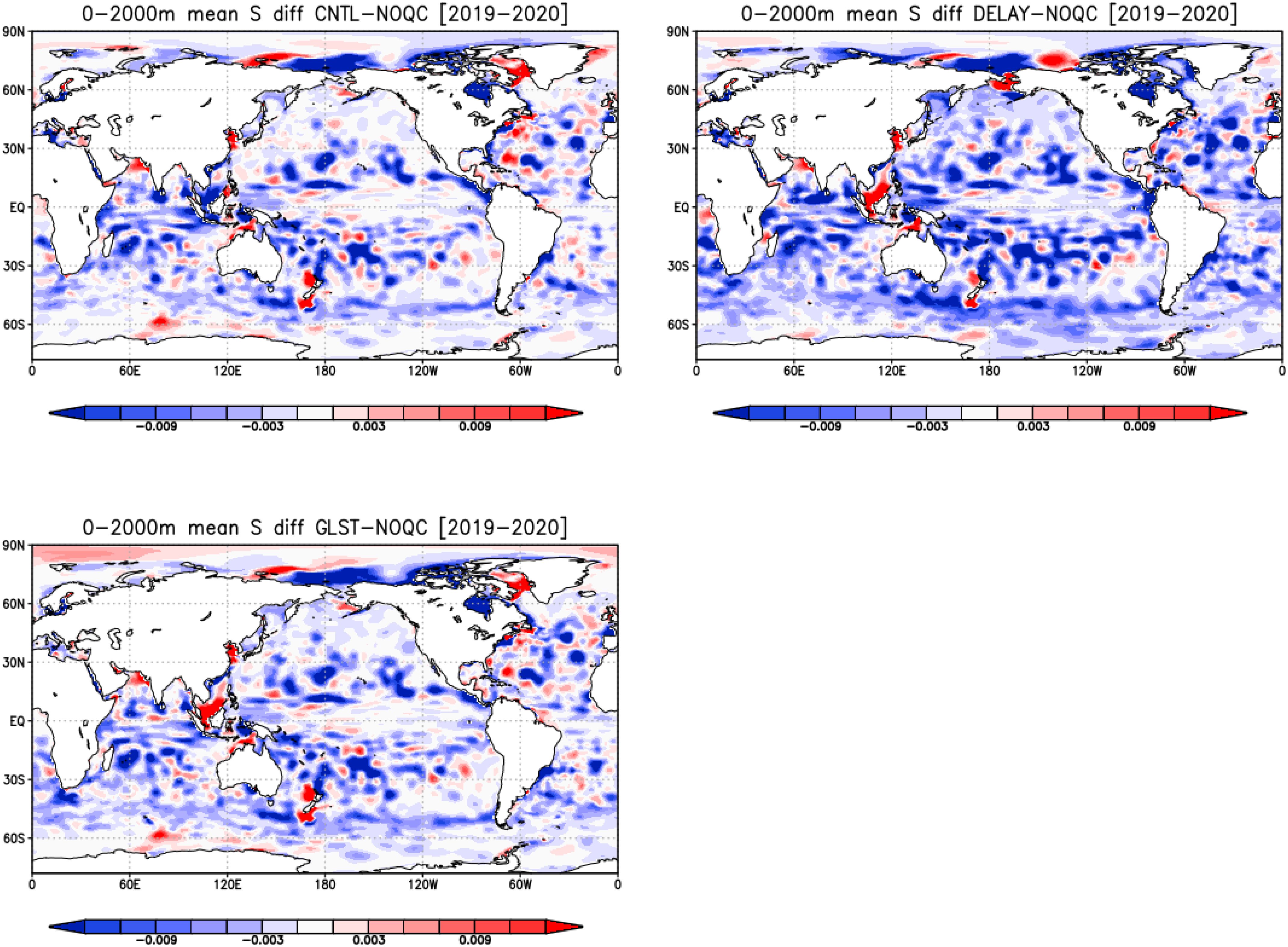
Figure 5. Horizontal distribution of differences in 0-2000m mean salinity in 2019-2020 of CNTL (top-left), GLST (bottom), and NOQC (top-right) compared to DELAY from MOVE-G3A.

In order to examine the QC impacts on the analysis quality, the root-mean-square difference (RMSD) of the analyzed salinity values relative to the Argo observations used in DELAY is calculated at each level in 10°×5° (zonal×meridional) boxes for each MOVE-G3A’s OSEs. Differences of the RMSD among the OSEs are shown in Figure 6. The figure indicates that the RMSD decrease of the DELAY from NOQC is generally larger than the decrease from CNTL and GLST, which suggests that the delayed-mode QC, including the corrections of spurious drifts of Argo salinity observations, has led to an improved analysis for 2019-2020.

Figure 6

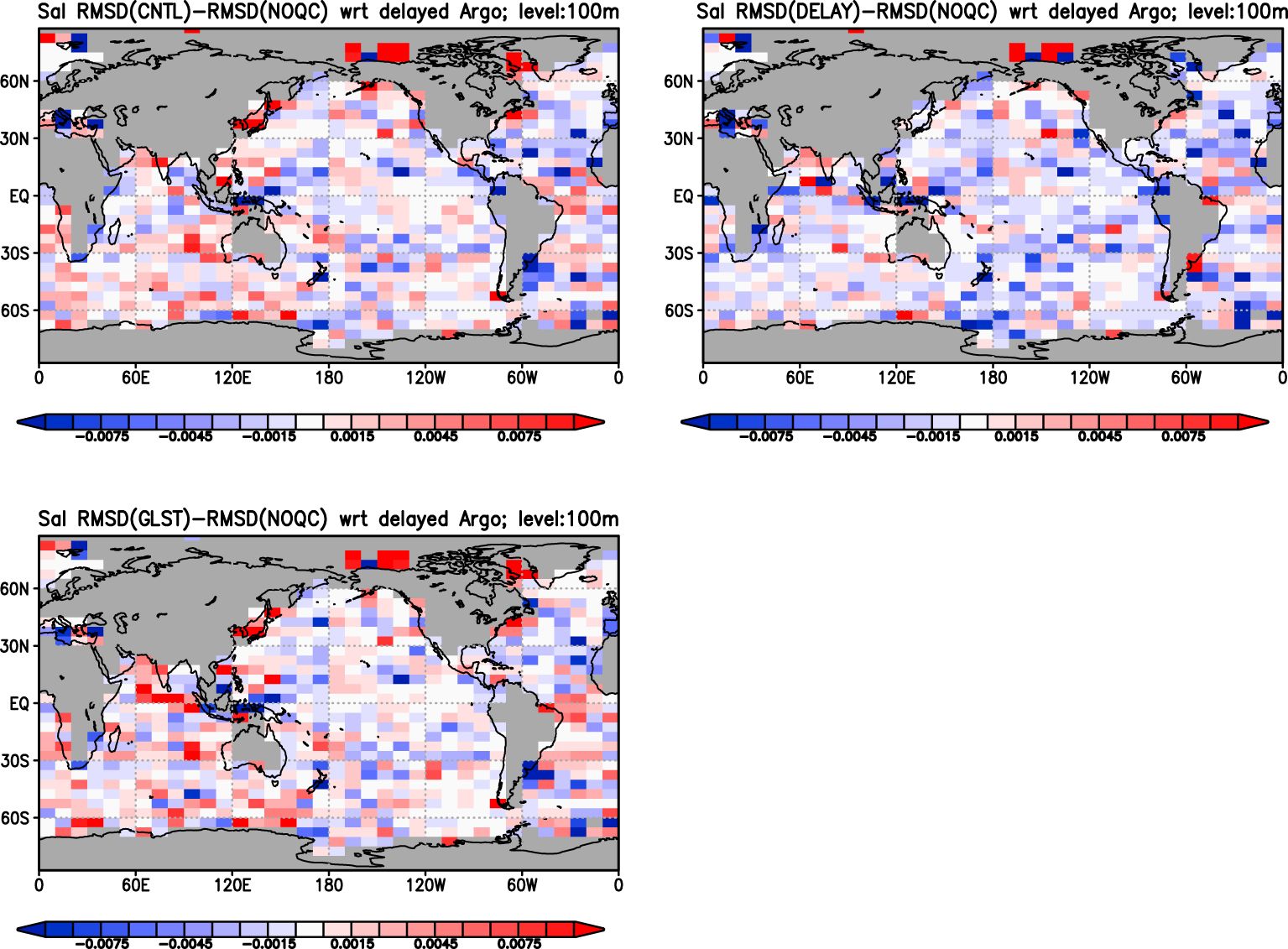
Figure 6. Difference of RMSDs of the MOVE-G3A salinity relative to the delayed-mode Argo float data (assimilated in DELAY OSE) between NOQC and each of the other OSEs at the 100m depth in the years from 2019 to 2020; upper-left: RMSD(CNTL)-RMSD(NOQC), upper-right: RMSD(GLST)-RMSD(NOQC), lower-left: RMSD(DELAY)-RMSD(NOAC). For this figure, the values of the ‘preparation run’ of MOVE-G3A, in which simultaneous observations have not yet been assimilated are used as the analysis. Blue colors mean that the RMSD is smaller than NOQC. Units in PSU.

We also calculate averages of analyzed salinity values at the locations of Argo observations at each level in the same 10°×5° boxes for each OSE, along with averages of observed salinity values used in each OSE for each box. Time-depth plots of changes from the first year (2015) of the global means of the box averages for salinity analyses and observations are shown in Figure 7. The figure indicates that the observed spurious increasing salinity trends seen below 150 m depth are reduced by QC, and it is indicated that the higher the QC level, the larger the correction to reduce the false salinity trends. Comparison among the OSEs of the global mean of the analyzed salinity at the sites corresponding to the observations indicates that the impact of the QC on the analysis generally reflects the differences in the input observations.

Figure 7

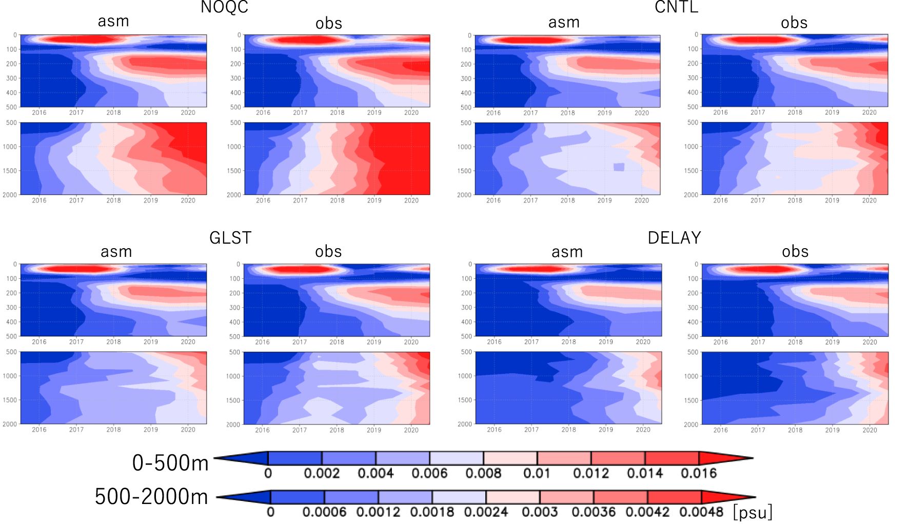
Figure 7. Analyzed and observed annual global mean salinity differences from the year 2015 plotted on the depth-time cross section for NOQC (upper-left), CNTL (upper-right), GLST (lower-left), and DELAY (lower-right). In each panel, left part shows analyzed values, and right part shows observed values. Note that the shallower levels than 500m are expanded vertically, and color scales are different from those at the deeper levels. Units in PSU.

3.2 Impacts of the QCs on the temperature field

This subsection investigates how the changes in the salinity field due to the Argo QCs affect the temperature field. As shown in Figure 8, the global mean ocean temperature has an increasing trend for all OSEs of all three systems. This trend is not considered spurious as for salinity because it is assumed that there is a real warming trend due partly to anthropogenic global warming. The trend represented by the OSEs seems plausible since the temperature increases over the six-year period by roughly 0.02-0.03°C in all the OSEs from the different systems. They are, however, significantly larger than the trend represented by the MOVE-G3A FREE. This discrepancy can be attributed to errors in the atmospheric forcing; for example, cloud processes, which play important roles in the Earth’s energy budget and have significant predictive uncertainty (Wong and Minnett, 2018; Liu et al., 2023), in the atmospheric reanalysis could lead to a bias in long-wave radiation at the sea surface. The possibility that the trend in the OSEs is excessive cannot be ruled out.

Figure 8

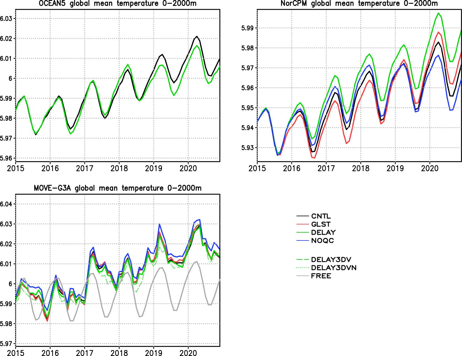
Figure 8. Same as Figure 2 but for the global mean temperature.

The differences of the global mean temperature among the different OSEs of a given system are much smaller than the difference between the OSEs and the FREE run from MOVE-G3A. Using Argo data with a more rigorous QC has only a minor impact on the warming trend. The OSEs with MOVE-G3A indicate that using the data with a rigorous QC generally reduces the warming trend slightly (Figure 8). NOQC indeed shows the highest temperature for almost the entire period, and differences among the other OSEs are relatively small. It is also true for OCEAN5, where the OSE (DELAY) with the more rigorous QC suppresses some of the warming trend compared with the other one (CNTL) with moderate QC. As for NorCPM, the order is opposite, that is, the DELAY OSE has the fastest warming trend and the NOQC has the slowest. The range of the warming trend for the NorCPM’s OSEs is greater than the range for the other two systems, which may have been influenced by the switch from anomaly assimilation to full-field assimilation, similar to what was noted for salinity.

The impacts on temperatures among the OSEs shown above may directly reflect the temperature observations, or may be affected by the salinity observations through the cross-covariance relationship in the data-assimilation systems. To investigate this point, Figure 9 compares the global mean temperature trends between the assimilation results and the observations in MOVE-G3A. The warming trends of analyzed temperatures in the OSE (DELAY) with the more rigorous QC are generally smaller than the other OSEs especially at the deeper levels, while the corresponding differences among the other OSEs is unclear. It should be noted that the observed temperature trends have no clear differences among the OSEs, but are generally smaller than those analyzed. It is thus suggested that the QC impacts on temperatures, which have been shown also in Figure 8, do not reflect changes in temperature observations directly. Since the data-assimilation procedure of MOVE-G3A uses amplitudes of the vertical coupled temperature-salinity EOF modes as control variables (Fujii and Kamachi, 2003; Usui et al., 2015), the impacts on assimilated temperatures can be affected by changes in salinity observations through the statistical TS relationship.

Figure 9

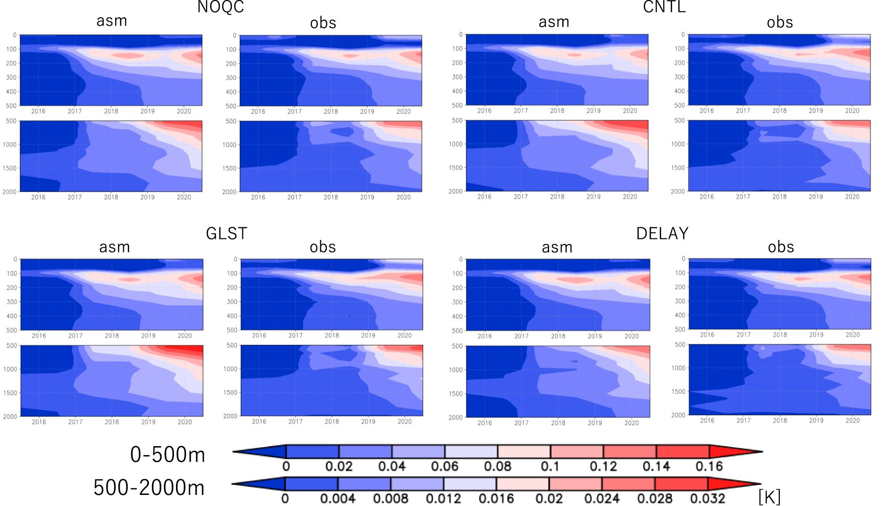
Figure 9. Same as Figure 7, except for temperature.

3.3 Impacts of the QCs on the steric height

Spurious salinity trends are expected to lead to errors in the estimated steric height variations. Sea-surface dynamic height (SDH) is a proxy for the steric height and can be estimated from the analyzed temperature and salinity fields (Fujii and Kamachi, 2003) in the ocean data assimilation system. Time-series of the global mean SDH relative to 2000 m depth in the OSEs with the MOVE-G3A are shown in Figure 10, along with the time series of the global means of the SSH and the steric height from satellite observations. Here, the global mean SSH is calculated from the CMEMS L4 sea level anomaly data (CMEMS, 2023b) and the global mean steric height is calculated by removing from the global mean SSH the global mean SSH change due to the change in the global water mass estimated from the gravity satellites (Landerer, 2022). It should be noted that the global mean SDH change is mostly equivalent to the global mean steric height change but the effects of the density change below 2000 m depth, which is included in the steric height change, is ignored.

Figure 10

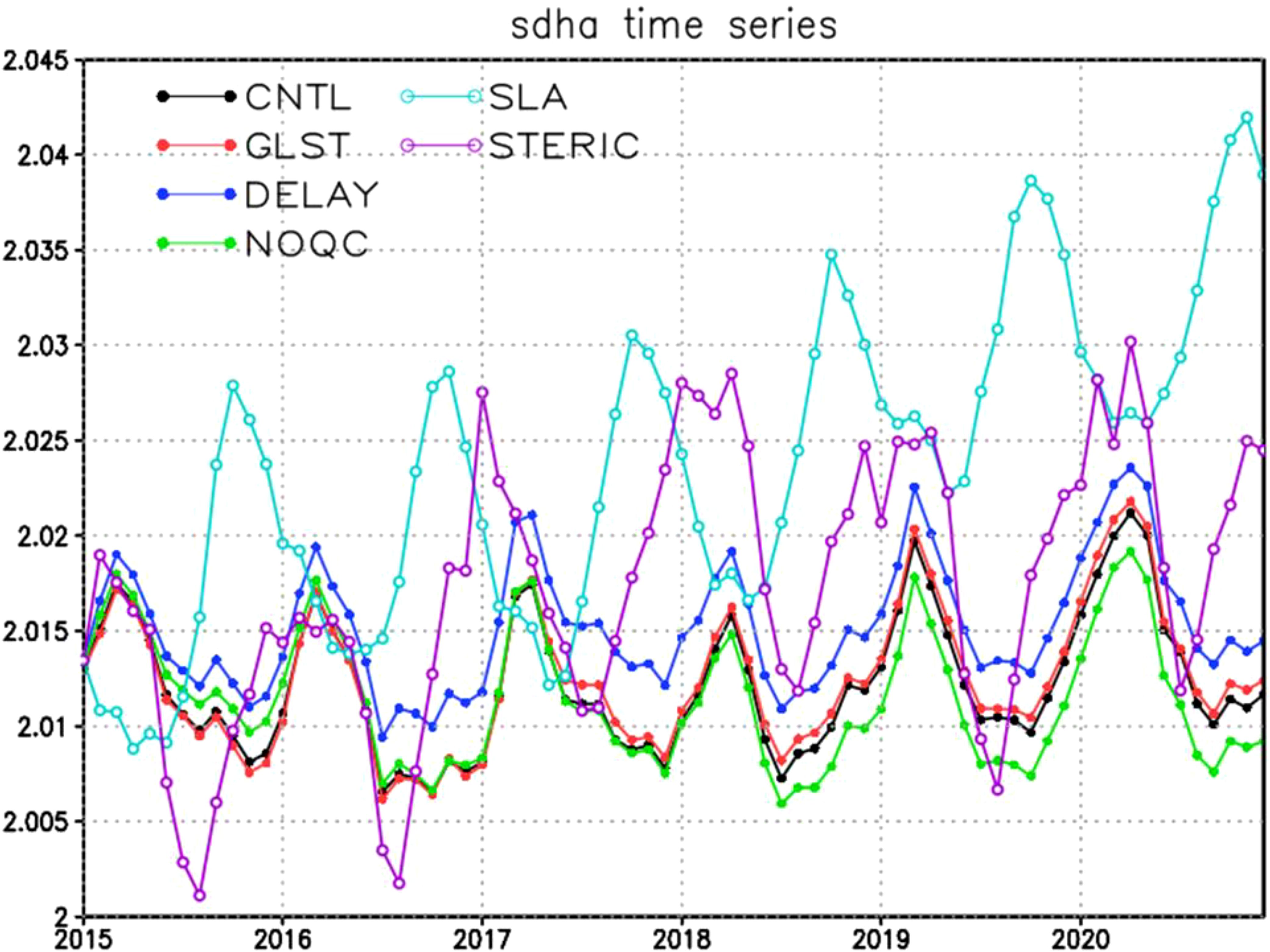
Figure 10. Time series of the global mean sea-surface dynamic height anomaly in CNTL (black), GLST (red), DELAY (blue), and NOQC (green); dynamic height is referenced to 2000m, and anomalies are differences from 2015-2020 average, seasonal variation not removed. Sea level anomaly (SLA) from the satellite altimetry (light blue), and estimated steric height anomaly (purple; SLA - fresh water input) are also plotted. SLA and estimated steric height anomaly are aligned to match the value of DELAY at the beginning of 2015.

While NOQC shows a decreasing trend in SDH, QC corrects it to an increasing trend, and DELAY especially shows an increasing trend, which is the nearest among the OSEs to the estimated steric height trend from satellite observations. While there is still a gap between assimilation results and satellite estimation regarding the magnitude of seasonal variation and interannual variability, it should be noted that the estimation is difficult because the SDH changes are out of phase between the southern and the northern hemispheres and are offset when global averages are taken. Lack of satellite SSH observations in the Arctic Ocean and the errors in the global water mass estimate are other factors causing this discrepancy.

QC impacts on SDH in MOVE-G3A OSEs are shown in Figure 11. Difference of SDH between CNTL and NOQC indicates that the real-time QC results in higher SDH over a wide area of the global ocean, especially in the South Indian Ocean due to the removal of high salinity bias by the QC. When Argo data with real-time QC are replaced by those with the delayed-mode QC, the increase in SDH is further spread globally, while impacts in the equatorial Pacific regions are relatively small. These features are consistent with impacts on salinity mentioned in Subsection 3.1 (Figure 5).

Figure 11

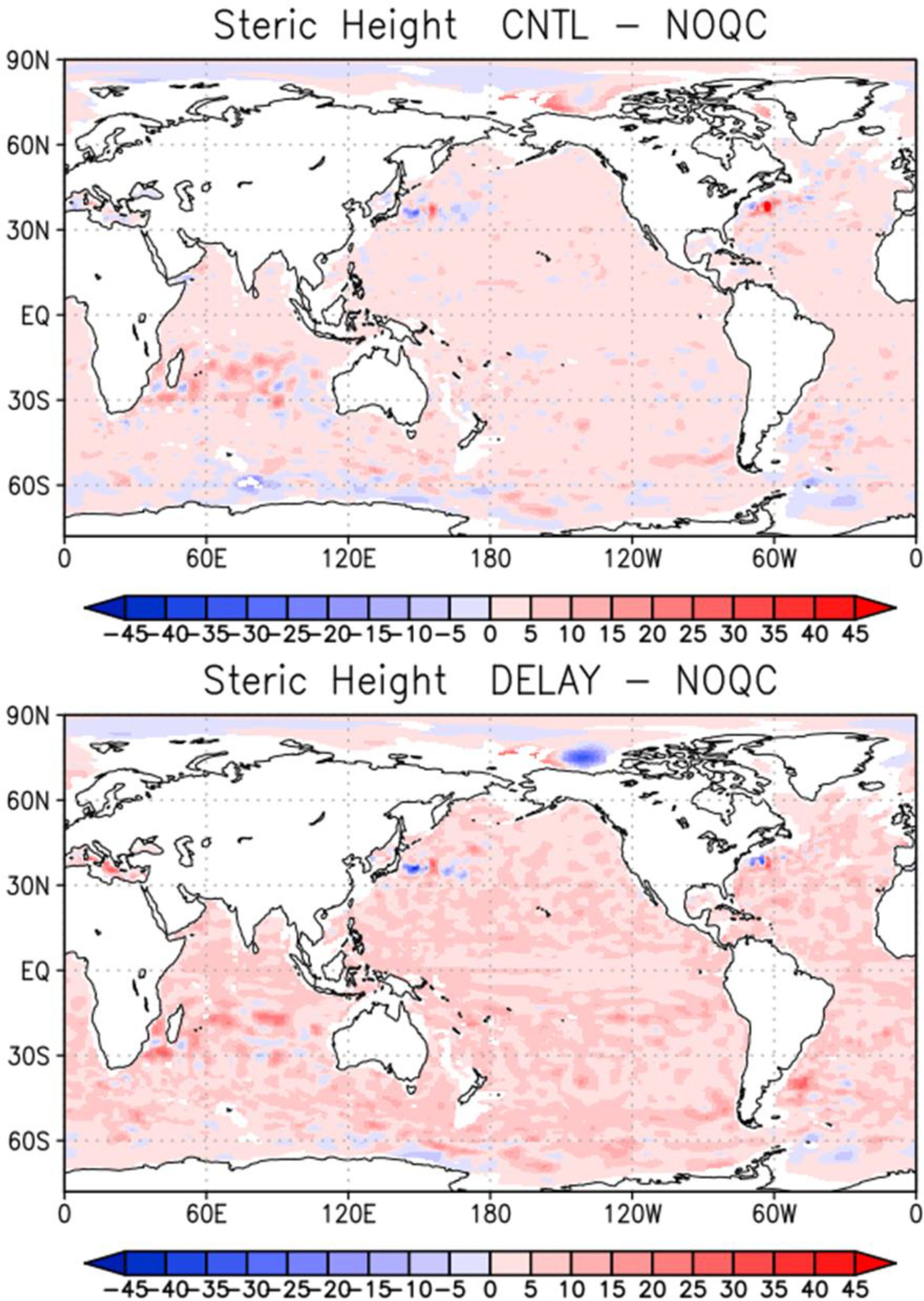
Figure 11. Differences of mean sea surface dynamic height during 2019-2020 between CNTL and NOQC (upper panel), and between DELAY and NOQC (lower panel). Units in cm.

QC impacts on the reproducibility of temporal variation of the steric height in the data assimilation are shown by the differences between the OSEs of the time correlations between the SDH and satellite steric height in each location in Figure 12. It should be noted that the pressure anomaly at 2000 m depth owing to the temperature and salinity variations in the deeper layer and the barotropic modes is counted in the satellite steric height but ignored in the SDH calculated from the OSE outputs. Real-time QC increases the correlations in large parts of the global ocean, and they are further increased by using the Argo data with the delayed-mode QC, especially in the Atlantic and South Pacific, although impacts in the equatorial Pacific are shown again to be relatively small. These results suggest that as a more rigorous QC is applied, the reproducibility of the steric height variations also improves through correction of both spurious positive salinity trend and other spurious salinity signals.

Figure 12

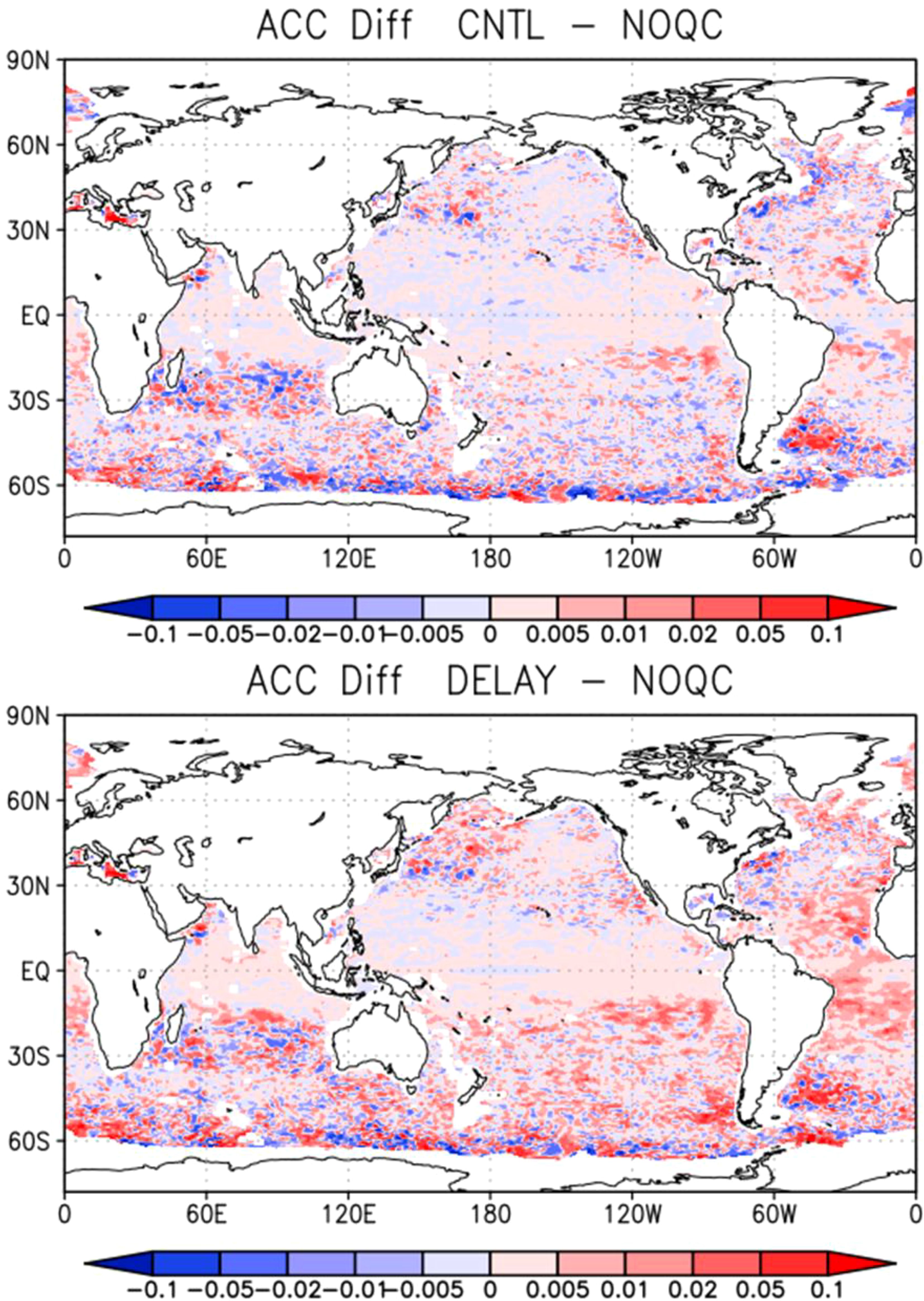
Figure 12. Differences between OSEs (upper: CNTL-NOQC; lower: DELAY-NOQC) of time correlations during 2015-2020 between SDHAs in ocean data assimilation and the steric height anomaly estimated from satellite altimetry.

4 Summary and discussion

Impacts of Argo data QC on the ocean data assimilation results are evaluated through OSEs with the multiple ocean assimilation systems, including the operational systems in JMA and ECMWF for seasonal forecast and ocean climate monitoring, and the BCCR system for climate predictions. Results show consistent QC impacts among the different systems on salinity analyses. The use of the raw data or the real-time data in the data assimilation systems results in an increasing trend of the global mean salinity, and the correction of the Argo data in the delayed mode QC acts to make the trend in the analysis smaller. Direct reflections on temperature analyses by correction to temperature observations are less clear in QC impacts, and analyzed temperatures can be affected by the correction to salinity observations through the statistical assumptions in the systems. In fact, MOVE-G3A results show that the higher the QC level, the lower the global mean temperature and salinity. As shown by the evaluation of analyzed sea-surface dynamic height compared with estimation from satellite altimetry, it is likely that the delayed mode QC of Argo data results in the improved temperature/salinity analyses, as a whole. The similarity of the QC impacts among three systems suggests little sensitivity to the characteristics of the ocean prediction system or the data assimilation scheme.

This study demonstrated the significant benefit of the QC conducted by the Argo DACs. However, it indicates that the real-time QC and application of the gray list are definitely not sufficient for a reliable estimate of the change in global mean ocean salinity. The increasing trend of the global mean salinity which remains in the OSE assimilating the data with the delayed-mode QC may suggest that even the delayed-mode QC does not completely eliminate systematic salinity observation errors because the global salt content is assumed to be more strictly conserved, as discussed later. On the other hand, this study clarifies that the QC incorporated in each ocean prediction system cannot avoid degradation by systematic errors sufficiently, and the support of the QC by the DACs was indispensable. However, it should be noted that QCs incorporated in ocean prediction systems can use information from ocean prediction results, which may have a potential to remove systematic errors more effectively. It is also desirable to provide ocean prediction outputs to the Argo DACs for more effective detection of systematic errors.

Since determination of the global ocean salinity trend remains a challenge, it is unclear how close to reality the result of the DELAY OSE has come. We can reasonably assume that changes in the global salt content are negligibly small, and a long-term increase in freshwater volume due to global warming should result in a decreasing trend in salinity. This is approximately the case for the global ocean shallower than 2000 m, assuming that the salinity exchange with the ocean deeper than 2000 m is small; the FREE experiment shows the small changes in global mean salinity for upper 2000m (Figure 2), meaning that the exchange is actually small in the model (the ocean model does not show a decreasing salinity trend, because the volume of the model ocean is essentially invariant). However, for a shorter period (e.g. 2015-2020), we cannot rule out the possibility that the global mean salinity actually increased.

Ponte et al. (2021) compared estimates of the global mean salinity based on the five different gridded salinity products derived from in situ measurements, and found that they showed little consistency in variability over various time scales. Ponte et al. (2021) also found an unrealistic increase in the global mean salinity after 2015 in all these products, except the Roemmich and Gilson (2009) reconstruction, in which stricter QCs are applied. The gravimetry (GRACE and GRACE-FO) based estimate in Ponte et al. (2021) showed a clear decreasing trend in global mean salinity, and much smaller seasonal and interannual variabilities than the estimates based on in-situ data. Bagnell and DeVries (2023) estimated salinity changes in the global ocean based on interpolated subsurface salinity data using an autoregressive artificial neural network, and they showed the similar trend and variability to the gravimetry based estimate. As Ponte et al. (2021) pointed out, better coverage of deep ocean, high latitudes, and ice-prone regions is expected to provide better consensus among various estimates of global ocean salinity, and gravimetry-based estimates may provide a way to calibrate the in situ estimates. In the future, it is important to expand the global ocean in-situ observation network below 2000 m, and to utilize satellite gravimetry data in order to reduce uncertainty in global ocean salinity estimation.

It should be also emphasized that careful monitoring of the ocean prediction outputs may help detect incidents occurring in the ocean observing system at an early stage. Indeed, one of the United Nations Ocean Decade Project, SynObs (Synergistic Observing Network for Ocean Prediction) promotes sharing information of ocean predictions among the ocean prediction and observation communities in the near-real-time, which is useful for monitoring the status of ocean observing networks. These communities are encouraged to be more co-operative in monitoring the status of ocean observing networks and responding immediately to incidents in ocean observing networks.

Data availability statement

The raw data supporting the conclusions of this article will be made available by the authors, without undue reservation.

Author contributions

II: Formal analysis, Investigation, Methodology, Software, Visualization, Writing – original draft, Writing – review & editing. YF: Conceptualization, Formal analysis, Funding acquisition, Investigation, Methodology, Project administration, Software, Visualization, Writing – original draft, Writing – review & editing. EB: Formal analysis, Investigation, Writing – original draft, Writing – review & editing. YW: Formal analysis, Investigation, Writing – original draft, Writing – review & editing. HZ: Formal analysis, Investigation, Writing – original draft, Writing – review & editing.

Funding

The author(s) declare financial support was received for the research, authorship, and/or publication of this article. For this work, YF was supported by ROIS-DS-JOINT (005RP2022, 029RP2023, and 027RP2024). YW was supported by the Research Council of Norway (Grant No. 301396) and the Trond Mohn Foundation under project number BFS2018TMT01. YW also received grants for computer time from the Norwegian Program for supercomputer (NN9039K) and storage grants (NS9039K). EB was supported by funds from the Copernicus Marine Service GLO-RAN project (21003-COP-GLORAN-LOT3). The publication fee is paid by JMA/MRI.

Acknowledgments

The authors thank Kanako Sato for providing information on the sensor failure of Argo floats.

Conflict of interest

The authors declare that the research was conducted in the absence of any commercial or financial relationships that could be construed as a potential conflict of interest.

Publisher’s note

All claims expressed in this article are solely those of the authors and do not necessarily represent those of their affiliated organizations, or those of the publisher, the editors and the reviewers. Any product that may be evaluated in this article, or claim that may be made by its manufacturer, is not guaranteed or endorsed by the publisher.

References

Adcroft A., Campin J.-M. (2004). Rescaled height coordinates for accurate representation of free-surface flows in ocean circulation models. Ocean Model. 7, 269–284. doi: 10.1016/j.ocemod.2003.09.003

Crossref Full Text | Google Scholar

Argo (2022). Argo float data and metadata from Global Data Assembly Centre (Argo GDAC). (France: SENOE). doi: 10.17882/42182

PubMed Abstract | Crossref Full Text | Google Scholar

Bagnell A., DeVries T. (2023). Global mean sea level rise inferred from ocean salinity and temperature changes. Geophys. Res. Lett. 50, e2022GL101004. doi: 10.1029/2022GL101004

Crossref Full Text | Google Scholar

Bentsen M., Bethke I., Debernard J. B., Iversen T., Kirkevåg A., Seland Ø., et al. (2013). The Norwegian Earth System Model, NorESM1-M – Part 1: Description and basic evaluation of the physical climate. Geosci. Model. Dev. 6, 687–720. doi: 10.5194/gmd-6-687-2013

Crossref Full Text | Google Scholar

Bethke I., Wang Y., Counillon F., Keenlyside N., Kimmritz M., Fransner F., et al. (2021). NorCPM1 and its contribution to CMIP6 DCPP. Geosci. Model. Dev. 14, 7073–7116. doi: 10.5194/gmd-14-7073-2021

Crossref Full Text | Google Scholar

CMEMS (2023a). Global ocean along track L 3 sea surface heights reprocessed 1993 ongoing tailored for data assimilation. Copernicus Mar. Service. doi: 10.48670/moi-00146

Crossref Full Text | Google Scholar

CMEMS (2023b). Global ocean gridded L 4 sea surface heights and derived variables reprocessed 1993 ongoing. Copernicus Mar. Service. doi: 10.48670/moi-00148

Crossref Full Text | Google Scholar

Donlon C. J., Martin M., Stark J., Roberts-Jones J., Fiedler E., Wimmer W. (2012). The operational sea surface temperature and sea ice analysis (OSTIA) system. Remote Sens. Environ. 116, 140–158. doi: 10.1016/j.rse.2010.10.017

Crossref Full Text | Google Scholar

Evensen G. (2003). The Ensemble Kalman Filter: theoretical formulation and practical implementation. Ocean Dynam. 53, 343–367. doi: 10.1007/s10236-003-0036-9

Crossref Full Text | Google Scholar

Fujii Y., Ishizaki S., Kamachi M. (2005). Application of nonlinear constraints in a three-dimensional variational ocean analysis. J. Oceanogr. 61, 655–662. doi: 10.1007/s10872-005-0073-8

Crossref Full Text | Google Scholar

Fujii Y., Kamachi M. (2003). A reconstruction of observed profiles in the sea east of Japan using vertical coupled temperature-salinity EOF modes. J. Oceanogr. 59, 173–186. doi: 10.1023/A:1025539104750

Crossref Full Text | Google Scholar

Fujii Y., Yoshida T., Sugimoto H., Ishikawa I., Urakawa S. (2023). : Evaluation of a global ocean reanalysis generated by a global ocean data assimilation system based on a four-dimensional variational (4DVAR) method. Front. Clim. 4. doi: 10.3389/fclim.2022.1019673

Crossref Full Text | Google Scholar

Good S. A., Martin M. J., Rayner N. A. (2013). EN4: Quality controlled ocean temperature and salinity profiles and monthly objective analyses with uncertainty estimates. J. Geophys. Res.-Ocean. 118, 6704–6716. doi: 10.1002/2013JC009067

Crossref Full Text | Google Scholar

Hirahara S., Kubo Y., Yoshida T., Komori T., Chiba J., Takakura T., et al. (2023). Japan meteorological agency/meteorological research institute coupled prediction system version 3 (JMA/MRI–CPS3). J. Meteorol. Soc. Jpn Ser. II 101, 149–169. doi: 10.2151/jmsj.2023-009

Crossref Full Text | Google Scholar

Hunke E. C., Lipscomb W. H. (2006). CICE: The Los Alamos Sea Ice Model Documentation and Software User’s Manual. Available online at: https://github.com/CICE-Consortium (Accessed August 1, 2024).

Google Scholar

Kosaka Y., Kobayashi S., Harada Y., Kobayashi C., Naoe H., Yoshimoto K., et al. (2024). The JRA-3Q reanalysis. J. Meteorol. Soc Jpn. Ser. II 102, 49–109. doi: 10.2151/jmsj.2024-004

Crossref Full Text | Google Scholar

Kurihara Y., Sakurai T., Kuragano T. (2006). Global daily sea surface temperature analysis using data from satellite microwave radiometer, satellite infrared radiometer and in-situ observations. Weather Service Bull. 73, s1–s18.

Google Scholar

Landerer F. (2022). GRACE/GRACE-FO Level-4 Monthly Global Ocean Mass Anomaly version 01 from NASA MEaSUREs HOMaGE project (CA, USA: PO.DAAC) (Accessed July 26, 2024).

Google Scholar

Liu H., Koren I., Altaratz O., Chekroun M. D. (2023). Opposing trends of cloud coverage over land and ocean under global warming. Atmos. Chem. Phys. 23, 6559–6569. doi: 10.5194/acp-23-6559-2023

Crossref Full Text | Google Scholar

Madec G. (2008). NEMO ocean engine, Note du Pôle de modélisation Vol. 27 (France: Institut Pierre-Simon Laplace (IPSL), 1288–1619.

Google Scholar

Mellor G. L., Kantha L. (1989). An ice-ocean coupled model. J. Geophys. Res.: Oceans 94, 10937–10954. doi: 10.1029/jc094ic08p10937

Crossref Full Text | Google Scholar

Mogensen K., Balmaseda M. A., Weaver A. (2012). The NEMOVAR ocean data assimilation system as implemented in the ECMWF ocean analysis for System 4, ECMWF Technical Memorandum, (United Kingdom: ECMWF) Vol. 668. 1–59. doi: 10.21957/x5y9yrtm

Crossref Full Text | Google Scholar

Murray R. J. (1996). Explicit generation of orthogonal grids for ocean models. J. Comput. Phys. 126, 251–273. doi: 10.1006/jcph.1996.0136

Crossref Full Text | Google Scholar

Nakano H., Suginohara N. (2002). Effects of bottom boundary layer parameterization on reproducing deep and bottom waters in a world ocean model. J. Phys. Oceanogr. 32, 1209–1227. doi: 10.1175/1520-0485(2002)032<1209:EOBBLP>2.0.CO;2

Crossref Full Text | Google Scholar

Ponte P. M., Sun Q., Liu C., Liang X. (2021). How salty is the global ocean: weighing it all or tasting it a sip at a time? Geophys. Res. Lett. 48, e2021GL092935. doi: 10.1029/2021GL092935

Crossref Full Text | Google Scholar

Pujol M.-I., Faugère Y., Taburet G., Dupuy S., Pelloquin C., Ablain M., et al. (2016). DUACS DT2014: the new multi-mission altimeter data set reprocessed over 20 years. Ocean Sci. 12, 1067–1090. doi: 10.5194/os-12-1067-2016

Crossref Full Text | Google Scholar

Roemmich D., Gilson J. (2009). The 2004–2008 mean and annual cycle of temperature, salinity, and steric height in the global ocean from the Argo Program. Prog. Oceanogr. 82, 81–100. doi: 10.1016/j.pocean.2009.03.004

Crossref Full Text | Google Scholar

Toyoda T., Fujii Y., Yasuda T., Usui N., Ogawa K., Kuragano T., et al. (2016). Data assimilation of sea ice concentration into a global ocean–sea ice model with corrections for atmospheric forcing and ocean temperature fields. J. Oceanogr. 72, 235–262. doi: 10.1007/s10872-015-0326-0

Crossref Full Text | Google Scholar

Tsujino H., Nakano H., Sakamoto K., Urakawa S., Hirabara M., Ishizaki H., et al. (2017). Reference manual for the meteorological research institute community ocean model version 4. Tech. Rep. Meteorol. Res. Inst. 80. doi: 10.11483/mritechrepo.80

Crossref Full Text | Google Scholar

Usui N., Fujii Y., Sakamoto K., Kamachi M. (2015). Development of a four-dimensional variational assimilation system for coastal data assimilation around Japan. Mon. Weather Rev. 143, 3874–3892. doi: 10.1175/mwr-d-14-00326.1

Crossref Full Text | Google Scholar

Weaver A. T., Deltel C., Machu E., Ricci S., Daget N. (2005). A multivariate balance operator for variational ocean data assimilation. Q. J. R. Meteor. Soc 131, 3605–3625. doi: 10.1256/qj.05.119

Crossref Full Text | Google Scholar

Wong A. P. S., Gilson J., Cabanes C. (2023). Argo salinity: bias and uncertainty evaluation. Earth Syst. Sci. Data 15, 383–393. doi: 10.5194/essd-15-383-2023

Crossref Full Text | Google Scholar

Wong A. P. S., Wijffels S. E., Riser S. C., Pouliquen S., Hosoda S., Roemmich D., et al. (2020). Argo data 1999–2019: two million temperature-salinity profiles and subsurface velocity observations from a global array of profiling floats. Front. Mar. Sci. 7. doi: 10.3389/fmars.2020.00700

Crossref Full Text | Google Scholar

Wong E. W., Minnett P. J. (2018). The response of the ocean thermal skin layer to variations in incident infrared radiation. J. Geophys. Res. Ocean. 123, 2475–2493. doi: 10.1002/2017JC013351

Crossref Full Text | Google Scholar

Zuo H., Balmaseda M. A., Tietsche S., Mogensen K., Mayer M. (2019). The ECMWF operational ensemble reanalysis–analysis system for ocean and sea ice: a description of the system and assessment. Ocean Sci. 15, 779–808. doi: 10.5194/os-15-779-2019

Crossref Full Text | Google Scholar