Adaptation of global primary production model to the Greenland Sea conditions: parameterization and monitoring for 1998-2022

Phytoplankton are responsible for releasing half of the world’s oxygen and for removing large amounts of carbon dioxide from surface waters. Despite many studies on the topic conducted in the past decades, we are still far from a good understanding of ongoing rapid changes in the Arctic Ocean and how they will affect phytoplankton and the whole ecosystem. An example is the difference in net primary production modelling estimates, which differ twice globally and fifty times when only the Arctic region is considered. Here, we aim to improve the quality of Greenland Sea primary production estimates, by testing different versions of primary production model against in situ data and then calculating regional estimates and trends for 1998-2022 for those performing best. As a baseline, we chose the commonly used global primary production model and tested it with different combinations of empirical relationships and input data. Local empirical relationships were taken from measurements by the literature and derived from the unpublished data of Institute of Oceanology of Polish Academy of Sciences across the Fram Strait. For validation, we took historical net primary production ¹⁴C data from literature and added to it our own gross primary production O₂ measurements. Field data showed good agreement between primary production measured with ¹⁴C and O₂ evolution methods. From all the model setups, those including local chlorophyll a profile and local absorption spectrum best reproduced in situ data. Our modelled regional annual primary production estimates are equal to 346 TgC/year for the Nordic Seas region and 342 TgC/year for the Greenland Sea sector of the Arctic defined as 45°W-15°E, 66°33′N-90°N. These values are higher than those previously reported. Monthly values show a seasonal cycle with less monthly variability than previously reported. No significant increase or decrease in primary production was observed when studying regionally averaged trends. The accuracy of the selected here model setups to reproduce the field data in terms of Root Mean Square Difference is better than in the related Arctic studies. The improved primary production estimates strengthen researchers’ ability to assess carbon flux and understand biogeochemical processes in the Greenland Sea.

1 Introduction

The Greenland Sea is one of the most productive regions of the Arctic Ocean (Arrigo and van Dijken, 2011; Sakshaug, 2004), which means that changes in its ecosystem are likely to affect the fisheries of the Arctic region (Chassot et al., 2010; Steingrund and Gaard, 2005). In addition to that, here deep convective mixing takes place (Bashmachnikov et al., 2021; Rey et al., 2000), and large amounts of carbon are possibly transferred to the deep ocean, having a profound effect on the global carbon cycle (Hansell et al., 2009). Most of the atmospheric CO₂ uptake occurs as the Atlantic water is cooled on its way north along the Norwegian coast, and consequently, the Atlantic water contains a high anthropogenic CO₂ content (e.g., Olsen et al., 2006; Sabine et al., 2004; Vázquez-Rodríguez et al., 2009). According to recent work by Chierici et al. (2019), phytoplankton uptake of CO₂ played by far the most important role in the observed CO₂ change throughout the study area and explained up to 89% of the total CO₂ change.

However, correct quantification of phytoplankton uptake of CO₂ (where primary production plays a major part) is challenging in the area due to several environmental factors. The first factor to consider is the dynamic circulation, characterised by warm and saline Atlantic waters in the eastern part, cold and fresh Arctic waters in the western part, and the large frontal zone with eddies in between these two water masses (Rudels and Quadfasel, 1991; Johannessen et al., 1987), as seen in Figure 1. The second factor is the presence of sea ice that, by melting, influences water stratification and circulation. Formation of sea ice constrains light exposure and nutrient supply of phytoplankton, and its melting enhances it, having a profound effect on phytoplankton blooms (e.g., Cherkasheva et al., 2014; McLaughlin and Carmack, 2010; Skogen et al., 2007; Slagstad et al., 2011; Von Appen et al., 2021). This effect is especially pronounced in the marginal ice zone, which is known to be the localisation of the large phytoplankton blooms in the area (Alexander and Neinauer, 1981; Cherkasheva et al., 2014; Perrette et al., 2011). Recently, it was found that such blooms can even be widespread under the ice, making up a large percentage of total biomass, which cannot be tracked with satellite data (Ardyna and Arrigo, 2020; Ardyna et al., 2020). Such under-ice blooms were documented, for example, in the area along the north coast of Svalbard and two degrees north of it (Assmy et al., 2017).

Figure 1

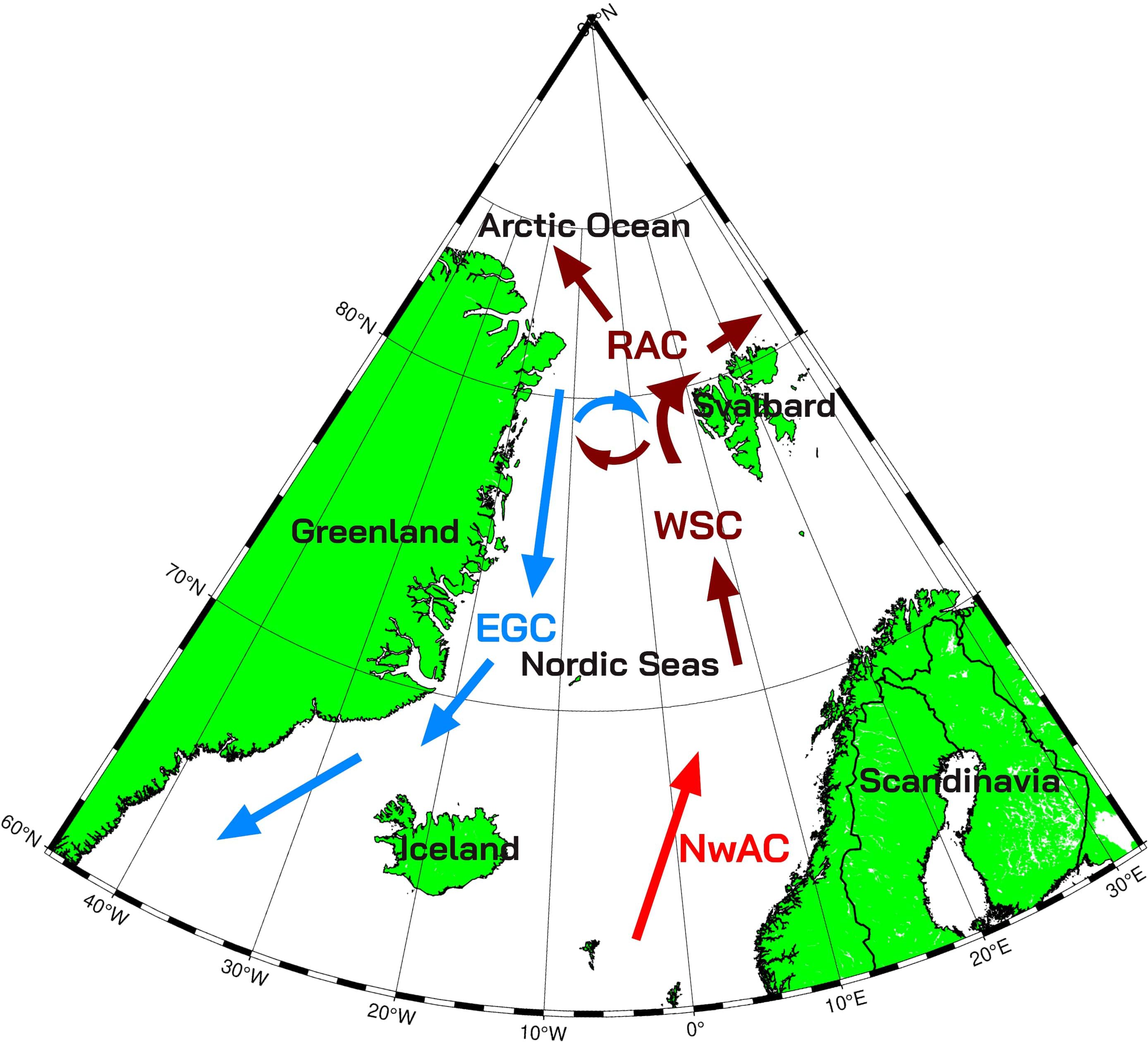
Figure 1. Schematic image of circulation patterns in the European Arctic. EGC, East Greenland Current; WSC, West Spitsbergen Current; NwAC, Norwegian Atlantic Current; RAC, Return Atlantic Current. Modified from Kraft (2013). Brown and red arrows denote warm water currents, and blue arrows denote cold water currents. The red arrow shows the warmest current in the area.

Another feature to be accounted for in the Arctic Ocean is often occurring deep subsurface chlorophyll maxima (SCMs) that significantly contribute to primary production (PP), but are mostly not detected by ocean colour sensors. In the context of current sea-ice loss in the Arctic, the role of SCM layer on biogeochemical fluxes will potentially increase, and this remains to be quantified (Ardyna and Arrigo, 2020). Commonly used models usually assume either uniform chlorophyll a (CHL) profile or global relationships between surface CHL and its profile (Antoine and Morel, 1996; Behrenfeld and Falkowski, 1997) with some exceptions (Ardyna et al., 2013; Cherkasheva et al., 2013).

Ocean colour PP models are also challenged in the Arctic Ocean by the limited availability of satellite and field data. The satellite data used as input to the models has large uncertainties and poor spatial coverage in the region due to specific conditions, such as low solar elevation, presence of sea ice (IOCCG, 2015), and extensive presence of clouds in summer (Eastman and Warren, 2010; Intrieri et al., 2002). The coverage of field data that could be used for validation is also limited. We have checked the availability of PP data for the satellite era with continuous ocean colour time series (1998-2022, after the SeaWiFS launch) in the largest field primary production database for the Arctic region ARCSS-PP (Matrai et al., 2013). The percentage of primary production data for the Greenland Sea sector of the Arctic in the ARCSS-PP database is only 0.3% compared to the data from the whole Arctic region. While in terms of area (with land), the Greenland Sea Sector takes up 9% of the Arctic Ocean.

As a result of the above-mentioned factors, the quality of primary production modelling in the Arctic in general and in the Greenland Sea in particular still needs improvement. The most extensive assessment of the performance of primary production models is the series of studies called the Primary Production Algorithm Round Robin (PPARR), which uses a set of activities to compare PP models. According to one of the most cited PPARR studies, models estimating marine primary production range by a factor of two globally (Carr et al., 2006). If only the Arctic region is considered, the factor of difference increases to fifty (Carr et al., 2006). The most recent Arctic PPARR by Lee et al. (2015) showed that PP models need to be carefully tuned for the Arctic Ocean because most of the models that performed relatively well were those that used Arctic-relevant parameters (e.g. Belanger et al., 2013; Hirawake et al., 2012).

Taking into account these challenges, we have formulated the goals of the current article: 1) develop a model setup adapted for the Greenland Sea based on the global primary production model, 2) obtain more accurate regional primary production estimates, and 3) monitor the primary production variability for the period when ocean colour data are stably available (1998-2022).

2 Method and data

The overview of the procedure to choose the best-performing model setup and then calculate basin estimates is presented in Figure 2. The global primary production model equation was taken as a base (Morel, 1991), and then the different setups with the variations of the input parameters (from different satellites and climatologies) and the variations of the local parameterizations (from field data) were calculated. The resulting different setups of a model were then validated against the in situ data to choose the best-performing model setup. Finally, for the best-performing model setup, the basin estimates and temporal trends were calculated.

Figure 2

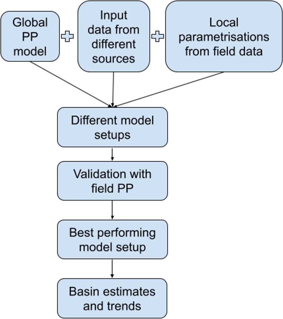
Figure 2. Scheme of the procedure applied to calculate Greenland Sea primary production basin estimates and trends.

2.1 Region

The spatial limits for the region of study were set at 45°W-15°E, 65°N-84°N for the results to be comparable with the studies of Hill et al. (2013) and Arrigo and van Dijken (2011) who calculated the basin primary production estimates for this part of the Arctic. All the data used were limited to the period of April-September 1998-2022.

2.2 Choice of a PP model

The choice of a PP model is not a straightforward task, as it was shown that no best model exists for all conditions (Saba et al., 2011). However, during one of the latest PPARR studies the Antoine and Morel (1996) model performed among the best models (in terms of lowest Root Mean Square Difference (RMSD) between in situ and modelled data) in eight out of ten regions that were studied (Saba et al., 2011). The conclusive recommendation of Saba et al. (2011) was that ‘in deeper waters, Antoine and Morel (1996) model might be an excellent choice’ and this encouraged our decision to use the Morel (1991) equation, which is in the base of Antoine and Morel (1996) model. We are aware that when the PPARR was conducted for the Arctic region, the Antoine and Morel (1996) model did not perform best, as opposed to the models with Arctic-specific coefficients (Lee et al., 2015). However, it is a model of depth-resolved type, which correlated more with in situ primary production than other model types (Lee et al., 2015) and has high potential globally. We were not able to use Antoine and Morel (1996) model as its components, i.e. look-up tables are not available online; therefore, here we applied a simplified version of Morel (1991) model adding to it the Arctic-specific coefficients.

The main equation of the Morel (1991) simplified case model, which is a wavelength-integrated depth-resolved primary production model is the following:

$\begin{array}{ll}P=(\frac{12}{4.6})CH{L}_{tot}\overline{PAR}(0^{+})\overline{a^{*}{\phi }_{\mu }}& (1)\end{array}$

For the baseline, we took values of spectrally-averaged constant CHL-specific absorption coefficient (a*), and average quantum yield valid for the euphotic layer ($\overline{{\phi }_{\mu }}$) from Morel (1991). $CH{L}_{tot}$, which is a total CHL integrated over the euphotic layer, was calculated from the surface CHL based on Morel and Berthon (1989) method. Following Morel and Berthon (1989), the model of Morel (1988) was used for the estimation of both $Z_{eu}$ (euphotic layer depth) and $CH{L}_{tot}$. 12 is the coefficient that transforms the net amount of carbon fixed from molC into mass by using the carbon molar weight (12 g/mol) and 4.6 is the coefficient accounting for the light attenuation with depth [for more details see Appendix 2 in Morel (1991)].

2.3 Input data

2.3.1 Satellite and reanalysis data

To calculate outputs for different model versions, seasonal basin estimates, and temporal trends, we have used the satellite data described in this section. For all satellite data, we’ve taken monthly composites, as for the daily or 8-day averages the coverage was much poorer. For example, for the whole Arctic, Lee et al. (2015) found only 85 match-ups between satellite and in-situ daily data, only two of which are in the Greenland Sea sector (visual analysis of Figure 1 in Lee et al. (2015)). Recognizing that phytoplankton concentrations can vary significantly within a month, we’ve tested the 8-day satellite data collocation with our primary production field dataset (see details in section 2.3.3 below) and got 13 match-ups for a dataset of 45 points, which was not sufficient from our point of view and supported our decision to perform the analysis on monthly data. The decision to test different satellite data products was also mainly based on the spatial availability of data for the test month of August 2022, since we faced the issue of most of the ocean colour data not being available for the latitudes higher than 78°N in our region of study. The test month of August 2022 was chosen based on the most recent expedition with available field data.

For satellite CHL we have used Copernicus-GlobColour Level 4 CHL (SeaWiFS, MODIS, MERIS, VIIRS-SNPP & JPSS1, OLCI-S3A & S3B) monthly and interpolated data (resolution: 4 km) and Globcolour Level 3 CHL (MERIS, MODIS, VIIRSN) for monthly data from Case1 waters (resolution: 4 km). Copernicus-GlobColour CHL for the test month showed 83% coverage, while Globcolour CHL showed 69% coverage.

For Photosynthetically Available Radiation (PAR) we have used Eumetsat OLCI Level 2 PAR daily data, which we combined into monthly composites (resolution: 1200 m at nadir) and Globcolour Level 3 MODIS/VIIRSN merged PAR monthly product (resolution: 4 km). Eumetsat PAR for the test month showed 87% coverage, while Globcolour PAR showed 81% coverage. For OLCI Level 2 PAR data for all the months from April until September were available only for 2022, thus we took 2022 data and regarded it as climatology for further calculations. As an alternative for the satellite PAR data, we used reanalysis climatological estimates. Reanalysis estimates that incorporate observations and numerical simulations with data assimilation of monthly average downward solar radiation flux at ~1.9° resolution were obtained from NOAA/National Centers for Environmental Prediction and converted to PAR by multiplying by C=0.43, PAR to the shortwave radiation fraction (Olofsson et al., 2007).

As for the accuracy of the mentioned satellite data, though the Arctic Region is challenging for optical remote sensing measurements, the global CHL remote sensing algorithms were adjusted for Arctic Ocean waters (Cota et al., 2004) with an acceptable result. For example, the OC4L algorithm applied to Western Arctic Ocean shelf waters characterized by strong CDOM absorption, retrieved CHL with the requisite accuracy for this parameter (RMSD < 35%) (Matsuoka et al., 2007). Satellite-derived PAR data validation in the Arctic also previously showed a generally good agreement between satellite-derived estimates and ship-based data and between methods (Laliberté et al., 2016).

2.3.2 Field data used for local coefficients

For the local dependency between satellite CHL and vertical CHL profile we’ve used already existing vertical CHL parameterization for the Greenland Sea based on analysis of 1199 profiles from Cherkasheva et al. (2013). The dataset used in Cherkasheva et al. (2013) covers months from April to September for 1957-2010 for the region north of the Arctic circle at 66°33′39′′ N and between 45° W and 20° E. The mathematical approximations of CHL profiles were obtained by Cherkasheva et al. (2013) by applying a Gaussian fit to the median monthly resolved chlorophyll profiles for the several categories defined by surface CHL. For the calculation of local a* made in the current paper we’ve used particulate absorption data and CHL data further described in the sections 2.3.2.1 and 2.3.2.2.

2.3.2.1 Particulate absorption data

For the particulate absorption database, we combined the measurements obtained during the cruise to the Fram Strait onboard of RV ‘Kronprinz Haakon’ in 2021 and data from Kowalczuk et al. (2019) for 2014-2016 from the same area.

Samples for particulate absorption analyses were taken from three depths at selected stations (5, 15, and 25 m) and filtered onto 0.7 µm glass fibre filters (Whatman, GF/F). The filters were stored at -80°C freezer and analysed at the home laboratory of the Institute of Oceanology of Polish Academy of Sciences (IOPAN). The absorbance of the particles deposited on the filter paper was measured with Lambda 850 (Perkin Elmer, USA) in the spectral range 300 - 850 nm with 1 nm resolution, equipped with the integration sphere using the transmission-reflection method described by Tassan and Ferrari (2002), and Tassan and Ferrari (1995). The phytoplankton pigment absorption coefficient, a_ph(λ), was calculated using the standard procedure described in Kowalczuk et al. (2019). The CHL-specific phytoplankton pigments absorption coefficient at 443 nm, a^*ph(443), was calculated for a given sample as the ratio of a_ph(443) to CHL concentration (Bricaud et al., 1995).

2.3.2.2 Chlorophyll a data

The pigments contained in the suspended particles retained on filter pads were extracted in 96% ethanol at room temperature for 24 hours (Wintermans and De Mots, 1965; Marker et al., 1980). CHL concentration was determined using a spectrophotometric method (Lorenzen, 1967) using a Perkin Elmer Lambda 650 spectrophotometer. The optical density OD(λ) of the pigment extract in ethanol was measured in a 2 cm cuvette. The raw OD readings at 665 nm were corrected for the background signal in the near-infrared region (750 nm): ΔOD = OD(665nm) - OD(750nm); and the resulting OD was converted to CHL concentration using an equation involving the volumes of filtered water (Vw) and the ethanol extract (VEtOH), the path length (l), and the specific absorption coefficient of CHL in 96% ethanol at 665 nm (Strickland and Parsons, 1972; Stramska et al., 2003):

$\begin{array}{ll}CHL=({10}^3\mathrm{\Delta }OD*V_{EtOH})/(83V_w*l)& (2)\end{array}$

2.3.3 Field data used for validation

Due to the limited availability of publicly available field primary production data in the region (Section 1), for validation, we have used data obtained with two different methods: net primary production data obtained with the ¹⁴C method (Steemann Nielsen, 1952) (NPP_C14) (see Section 2.3.3.1), and gross primary production obtained with optode O₂ measurements (GPP_O2) (see Section 2.3.3.2).

2.3.3.1 Net primary production data with ¹⁴C measurements

For our region of study for 1998-2022, five points were available from the Matrai et al. (2013) database, and 19 points from RV Dana and RV Triton cruises (Richardson et al., 2005). We have also added nine data points from the two Spitsbergen fjords (Iversen and Seuthe, 2011; Piwosz et al., 2009). As a result, we got a total of 33 data points for the period of April-September 1999-2006. The data by Richardson et al. (2005) were taken from two depths: the surface and the SCM (varying depth), samples were incubated in the incubator for 24 hours at a temperature +1˚C. Fjords data by Iversen and Seuthe (2011) were collected for the six depths down to 50 m, the samples were incubated overboard for 24 hours. Another fjords dataset by Piwosz et al. (2009) also has the data incubated in the sea for the six depths down to 50 m, with incubations lasting 6-9 hours at midday and then extrapolated to daily measurements, For the Matrai et al. (2013) dataset, data were collected from four to seven depths down to 50m. No information on the incubation procedure was found in the metadata files. For all the datasets, in case the data contained only vertically integrated values we used them without processing, in the cases when depth-resolved data was available, we integrated the values till the last available depth

2.3.3.2 Gross primary production with optode O₂ measurements

These are data obtained and measured specially for this study during RV ‘Kronprinz Haakon’ 2021 Fram Strait cruise and RV ‘Maria S Merian’ 2022 Greenland Fjords cruise. This dataset has 13 points for August 2021-2022.

The estimation of gross primary production from the optode O₂ measurements was derived with the method adapted from Campbell et al. (2016) and also described in Section 6 of the Balch et al. (2022). The incubation bottles were overfilled with the seawater sample to prevent the formation of a headspace during the closure of the glass stopper and placed into containers with seawater under continuous illumination with an artificial lamp and mixing. The incubation temperature in the cold room was set at 4°C, which was representative of the average conditions of the seawater in situ in the area for the sampling layer (ranging from -2°C to 7°C). The determination of the gross primary production by oxygen modification was carried out with the help of oxygen measurements obtained using a Fixbox4 optical sensor (PreSens HMbH, Germany), which non-invasively utilises optical oxygen sensor spots installed in the 250 ml white glass bottles. Oxygen respiration was determined in foil-wrapped bottles of the same volume with the same optical sensor. The bottles were incubated in a thermostabilised luminostate at light levels representing surface, 15 m and 25 m PAR in the case of a 2021 cruise and surface, 40 m and 60 m in the case of a 2022 cruise (Figure 3). The depths were defined by the historical Fram Strait transect of the Norwegian Polar Institute which was not subjected to change in case of 2021 cruise and mutual agreement between the participating scientific groups in case of 2022 cruise. Each of the bottles had a duplicate in case of the 2021 cruise and a triplicate in case of the 2022 cruise. The light level reproducing surface light conditions was selected at the beginning of the cruise by choosing the light intensity of the lamp and the appropriate level of the neutral density film. The selection was made by visually comparing the measurement of downwelling irradiance spectra on deck with the hyperspectral irradiance sensor RAMSES ACC (TriOS, Germany), and the measurements of the different combinations of light intensity and neutral density film with the same downwelling irradiance spectra sensor in the cold room inside the incubation box. The light levels were assumed to be constant throughout the day, as both of the cruises took place in the beginning of August above 70°N in the period of the midnight sun at these latitudes. The oxygen concentration dynamics was determined every 6 hours for 24, 48, or 72 hours depending on the initial CHL concentration. The observed CHL concentrations were quite low (0.27 mgCHL/m³ on average for the surface samples), causing a longer incubation period from 48 to 72 hours than the standard 24 hours used for higher CHL concentrations. Samples of the same Niskin bottles were filtered for CHL measurements in parallel with oxygen incubations. Optode sensors were calibrated for bottles in use prior to the cruise using 0% and 100% dissolved oxygen standards of nitrogen-saturated water and oxygen-saturated water, respectively.

Figure 3

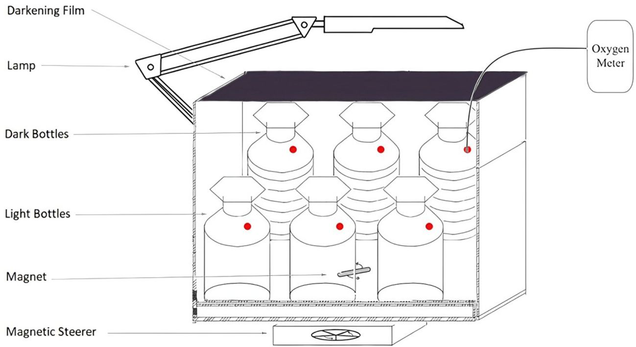
Figure 3. Gross Primary Production Measurements Setup during the Kronprinz Haakon Fram Strait 2021 and Maria S Merian 2022 cruises. Three of such boxes were installed, one for each depth.

After measurements were done, the values were averaged for duplicates in the case of the 2021 cruise and triplicates in the case of the 2022 cruise. Then, the rates of change of oxygen in dark bottles (an estimate of community respiration, CR, which is a sum of autotrophic respiration (AR) and heterotrophic respiration (HR)) and that in clear bottles (an estimate of net community production, NCP) were calculated by subtracting initial dissolved oxygen concentrations from the dissolved oxygen concentrations measured after incubation under dark and light conditions, respectively (Carritt and Carpenter, 1966; Carpenter, 1995). GPP was derived by summing NCP and CR (Carritt and Carpenter, 1966; Duarte et al., 2011). The relation between GPP, NCP, NPP, AR, and HR is summarised in the following equation (Li and Cassar, 2016):

$\begin{array}{ll}C{O}_2+H_{2}O \overrightarrow{\stackrel{GPP}{\overbrace{\underset{NPP}{\underbrace{\overrightarrow{NCP}\overleftarrow{HR}}}\overleftarrow{AR}}}}OrganicMatter+O_2& (3)\end{array}$

This equation defines GPP as a sum of NCP, AR, and HR, and NPP as a sum of NCP and HR.

In case the measurements were taken for 48 or 72 hours, they were weighted by the incubation time to achieve a value of 24 hours. Then, to convert the O₂ production rates into ¹⁴C incorporation rates, the specific photosynthetic quotient (PQ) value was used. Although no PQ value has been derived for the Arctic Ocean, a value of 1.25, proposed by Williams et al. (1979), has been widely applied in this region to convert O₂ molar stoichiometry units into C (i.e., Duarte and Agustí, 1998, Sanz-Martin et al., 2019, Vaquer-Sunyer et al., 2013). Therefore, we have used a PQ value of 1.25 and then integrated the data for the 2021 and 2022 cruises till the deepest depth available in 2021, which is 25m. To be informed on the effect of choosing a certain PQ value, we’ve additionally tested PQ values of 1.0 and 1.4 as the minimum and maximum values used for the ocean (e.g. Sanz-Martin et al., 2019; Balch et al. (2022) on the model performance.

2.4 Versions of primary production model setup

After the baseline equation (1) was set, there were several variations of the components of the model that we have tested when validating the model output against field PP data (Table 1).

Table 1

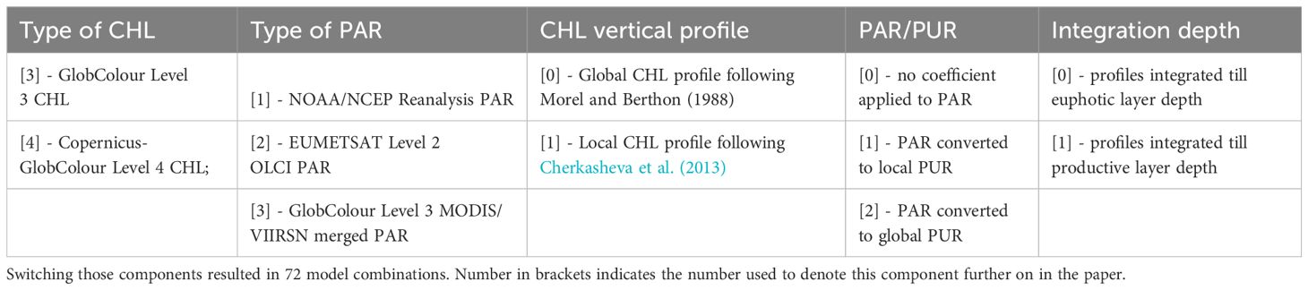
Table 1. Summary of the model components tested.

The groups tested were:

a. Source of CHL data (see Section 2.3.1 above):

1. Hermes ACRI Globcolour Level 3 CHL (CHL_L3)

2. Copernicus-GlobColour Level 4 CHL (CHL_L4)

b. Source of photosynthetically active radiation data (see Section 2.3.1 above):

1. NOAA/NCEP Reanalysis PAR (PAR_R)

2. EUMETSAT Level 2 OLCI PAR (PAR_L2)

3. Hermes ACRI Globcolour Level 3 MODIS/VIIRSN merged PAR (PAR_L3)

c. Shape of CHL vertical profile calculated using:

1. Global relationship between surface CHL and CHL profile used in Antoine and Morel (1996) model which is the satellite data adapted version of Morel (1991) model. Either uniform or Morel and Berthon (1989) shape of the profile was assumed; the distinction between the two cases was made based on latitude (for high latitudes >70°N the profile is assumed to be uniform) or on the mixed layer depth position. If the mixed layer depth was larger than 100 m or exceeded the euphotic depth, the profile was also assumed to be uniform (Antoine et al., 1996). The mixed layer depth values were taken from Boyer et al. (2018) climatology data. Previously Morel and Berthon (1989) was shown to capture only the early months of the Greenland Sea season (April-June, Cherkasheva et al., 2013), suggesting the need to use the monthly resolved relationship for the region as one in the next point (PROFILE_GLOB)

2. Local Greenland Sea relationship between surface CHL and CHL profile developed based on the analysis of 1199 profiles (Cherkasheva et al., 2013) (PROFILE_LOC)

d. The fraction of light spectrum. We have tested:

1. Photosynthetically Available Radiation (PAR) used in the majority of primary production models (e.g., Lee et al., 2015) and Morel (1991) simplified model version (SPECTR_PAR)

2. Photosynthetically Usable Radiation (PUR) used in Antoine and Morel (1996), which is a fraction of PAR absorbed by phytoplankton (Morel, 1978), is used instead of PAR in the equation (1). In this case the term “PAR” is substituted by the term “PUR”. To obtain PUR we multiplied PAR by a mean CHL-specific absorption spectrum computed from measurements for 14 phytoplankton species, grown in culture, and normalised with respect to a maximum value (Morel, 1991) (SPECTR_PUR_GLOB)

3. PUR accounted for the Greenland Sea species of phytoplankton. To obtain this version of PUR, the PAR values were multiplied by the climatology of the mean CHL-specific absorption calculated from the unpublished data from RV ‘Kronprinz Haakon’ 2021 Fram Strait cruise and data from Kowalczuk et al. (2019) for 2014-2016 (see Section 2.3.2.1). The mean CHL-specific absorption value was computed as the spectrally averaged percentage of absorption related to maximum value, which was assumed to be 100%. As the measurements did not cover all the area, for each point of the grid the closest available value was taken. (SPECTR_PUR_LOC)

e. Integration depth. We have compared integration of CHL data for two depths:

1. Euphotic layer depth (Zeu) calculated using the Morel (1988) model following Morel and Berthon (1989), which was later confirmed by Morel and Maritorena (2001) (DEPTH_ZEU)

2. Depth of the ‘extended’ productive layer (D) which is defined by Zeu multiplied by 1.5. D was introduced by Morel (1991) as in some cases Zeu does not cover the subsurface CHL maximum, thus giving false estimates of the integrated CHL profile (DEPTH_D).

For comparison, we have also added to the further analysis 1) publicly available PP output of Global Ocean Colour (Copernicus-GlobColour), Bio-Geo-Chemical, L4 (monthly and interpolated) from Satellite Observations (1997-ongoing) based on Antoine and Morel (1996) algorithm, and 2) Behrenfeld et al. (1998) PP model based on Globcolour Level 3 CHL.

2.5 Statistical analysis for model performance assessment

Field PP data were matched with modelled PP data using two methods: 1) commonly used method of matching field data location with satellite cell, i.e. the matchup was considered valid if daily field data coordinates fell into corresponding 4 km x 4 km monthly satellite data cell. Cells with missing modelled PP data were excluded. 2) method to increase the number of collocations further on named as «interpolated»: field data location was matched with a satellite cell using the same criteria as described in point 1; if the modelled PP data was missing, it was interpolated using the scipy.interpolate.griddata linear interpolation in Python developed for unstructured scientific data with more than one dimension The interpolant is constructed by triangulating the input data, and on each triangle performing linear barycentric interpolation.

Model performance was assessed using $RMSD$ for each participating model version, where N is the number of observations:

$\begin{array}{ll}RMSD=\sqrt{\frac{1}{N}{\displaystyle \sum {}_{i=1}^N}{(logNP{P}_m(i)-logNP{P}_d(i))}^2}& (4)\end{array}$

, where NPP_m(i) is modeled NPP and NPP_d(i) represents in situ data for each sample i. Generally, the smaller a $RMSD$ value becomes, the better a model performs. The $RMSD$ consists of two components: 1) bias representing the difference between the means of in-situ and model data ($BIAS$), providing the measure of how well the mean is modelled;

$\begin{array}{ll}BIAS=\overline{logNP{P}_m}-\overline{logNP{P}_d}& (5)\end{array}$

and 2) unbiased $RMSD$ ($uRMSD$), providing the measure of how well variability is modelled.

$\begin{array}{ll}uRMSD=\sqrt{\frac{1}{N}{\displaystyle \sum {}_{i=1}^N}{((logNP{P}_m(i)-\overline{logNP{P}_m})-(logNP{P}_d(i)-\overline{logNP{P}_d}))}^2}& (6)\end{array}$

The target diagram (Jolliff et al., 2009) was used to visualise $BIAS$ (y-axis), $uRMSD$ (x-axis) and $RMSD$ (distance from a center) on a single plot. To plot a Target diagram, $BIAS$ and $uRMSD$ are normalized by the standard deviation of $logNP{P}_d$. Normalized bias ($BIA{S}^{*}$) is thus defined as:

$\begin{array}{ll}BIA{S}^{*}=BIAS/{\sigma }_d& (7)\end{array}$

Normalized $uRMSD$ ($uRMS{D}^{*}$) is defined as:

$\begin{array}{ll}uRMS{D}^{*}=\frac{uRMSD}{{\sigma }_d} (if {\sigma }_m>{\sigma }_d)=-\frac{uRMSD}{{\sigma }_d} (if {\sigma }_m<{\sigma }_d)& (8)\end{array}$

, where ${\sigma }_d$ is the standard deviation of $logNP{P}_d$ and model is the standard deviation of $logNP{P}_m$.

As an additional characteristic to assess the skill of the model, the Pearson correlation coefficient (r) was calculated. The closer r is to 1, the better a model version performs.

Skill statistics for all versions of the model normalized by the standard deviation are visually presented in the Target diagrams. The closer a model symbol is to the origin, the better a model performs.

As in Lee et al. (2015), model versions performing relatively better than the others were selected for further analysis using the two criteria: (1) bias was close to 0 (-0.1<bias<0.1), and (2) Pearson’s correlation coefficient (r) was greater than the model average (0.25).

2.6 Calculation of trends and basin estimates

To compare our estimates to previous studies, we calculated basin primary production for two regions (Figure 4). The first region was set according to Hill et al. (2013) and covered the Nordic Seas region of the EASE grid representation of the Arctic Ocean starting at 65°N. Each cell in the grid was 100 x 100 km. As in the versions of the EASE grid available online now the Nordic Seas region borders have changed compared to Hill et al. (2013) version, we have digitized the map from Hill et al. (2013) using WebPlotDigitizer v4.6. Hill et al. (2013) paper includes Nordic Seas annual PP basin estimates accounting for SCM, and pan-Arctic monthly estimates accounting for SCM. However, monthly estimates for the Nordic Seas do not include SCM influence, thus we similarly to the method used in the paper assumed an underestimation of 75% for the calculations without SCM and corrected for that. The second region was set as in Arrigo and van Dijken (2011) and Arrigo and van Dijken (2015) at 45°W-15°E, 65°N-84°N. Trends were calculated using least squares linear fit. Mind that for these calculations PP was not log-transformed as opposed to the previous section.

Figure 4

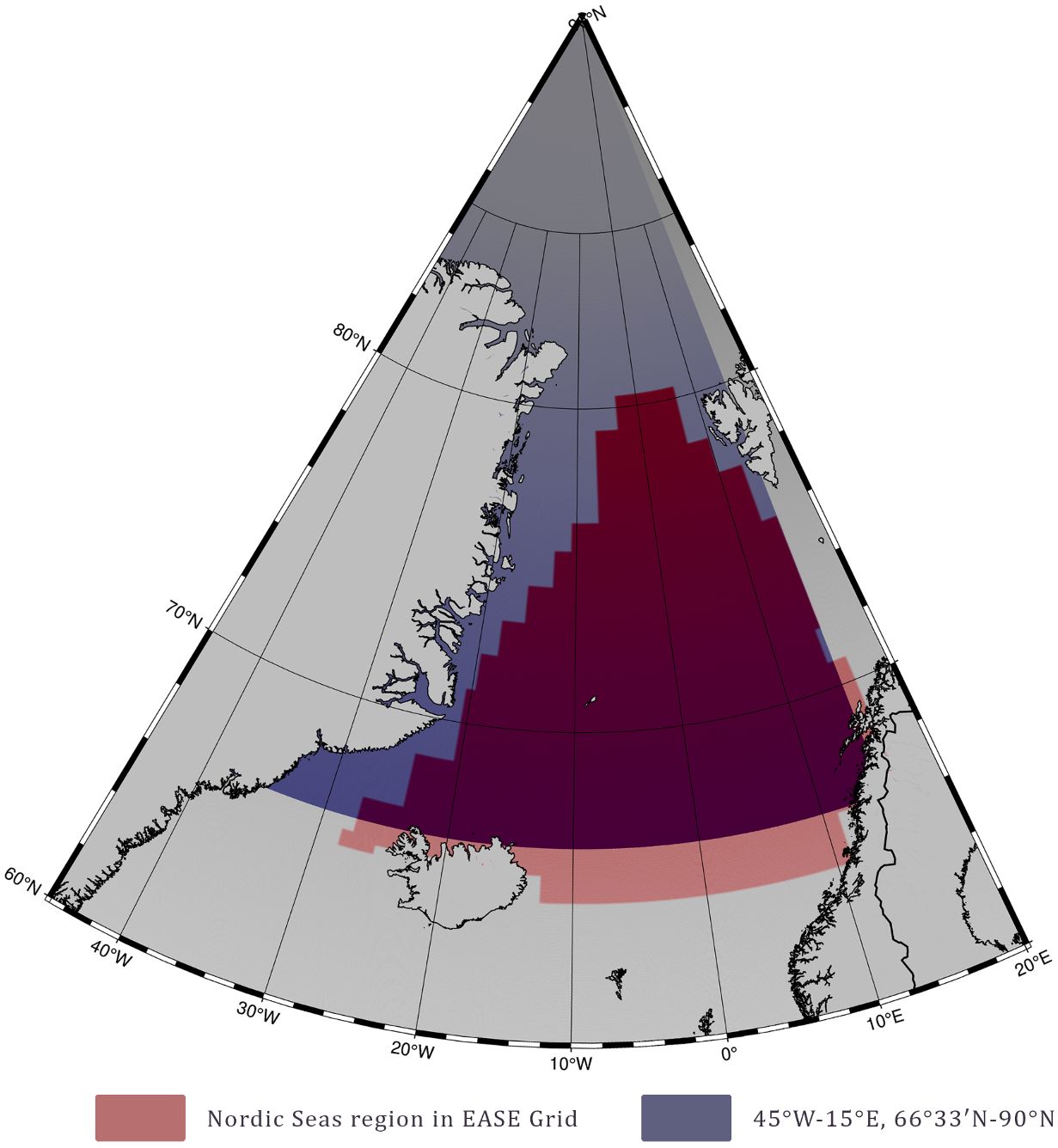
Figure 4. Two regions selected for the calculation of basin estimates for comparison with the of the PP model results from Hill et al. (2013) and Arrigo and van Dijken (2015).

3 Results

3.1 Field primary production data

Field primary production data were available for the period 1999-2006 for NPP_C14 and for the years 2021-2022 for GPP_O2. Looking at the spatial distribution of the field data in Figure 5, one can see the slightly larger values on the eastern Atlantic waters side as opposed to lower values on the polar waters side to the west.

Figure 5

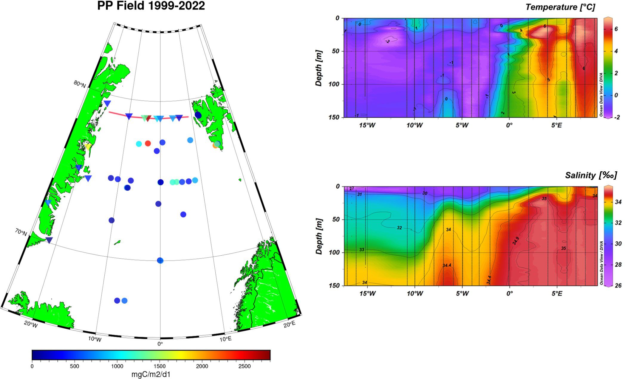
Figure 5. Left: Locations of field primary production data for 1999-2022 used for model validation. Circles indicate net primary production obtained with the ¹⁴C method for 1999-2006. Triangles indicate the gross primary production obtained with the dissolved O₂ method and converted to mgC/m²/day for 2021-2022. The red line shows the location of cross sections to the right. Right: Cross sections of temperature and salinity CTD measurements from the 2014 Fram Strait cruise across 79°N.

In between the polar waters and the Atlantic Waters lies a frontal zone. The location of the frontal zone can clearly be seen in the temperature and salinity cross section across the Fram Strait at 79°N in 2014 (Figure 5, right side). The location of this frontal zone is quite stable through the years, also confirmed, for example, by Granskog et al. (2012) and Gonçalves-Araujo et al. (2016). At the frontal zone (see area 76°N-80°N, 2°W-6°W on the map in Figure 5) both the NPP and GPP are larger, with maximum values observed in the area for both measurement methods.

These general patterns are in good agreement for both methods of data collection, although they were collected in different years and the type of measured primary production is different. The mean values of the data are 1.5 times higher for GPP_O2 - 884 mgC/m²/day for GPP_O2 and 589 mgC/m²/day for NPP_C14. The two-tailed hypothesis Student’s test gives a t-value of 1.53 and p-value of 0.06, showing the two datasets to be partially similar. The range of values is similar for both methods, being just slightly higher for the GPP_O2 values (Figure 6). In general, GPP_O2 is supposed to have higher values than NPP_C14 (e.g., Robinson et al. (2009), Balch et al. (2022)). In the literature comparisons between the GPP_O2 and NPP_C14 show on average a twofold difference between these two estimates in the Arctic, 21-70 mgC/m³/d for the surface 14C-NPP, and 55-168 mgC/m³/d for the surface GPP_O2 (Matrai et al., 2013; Sanz-Martin et al., 2019; Vaquer-Sunyer et al., 2013).

Figure 6

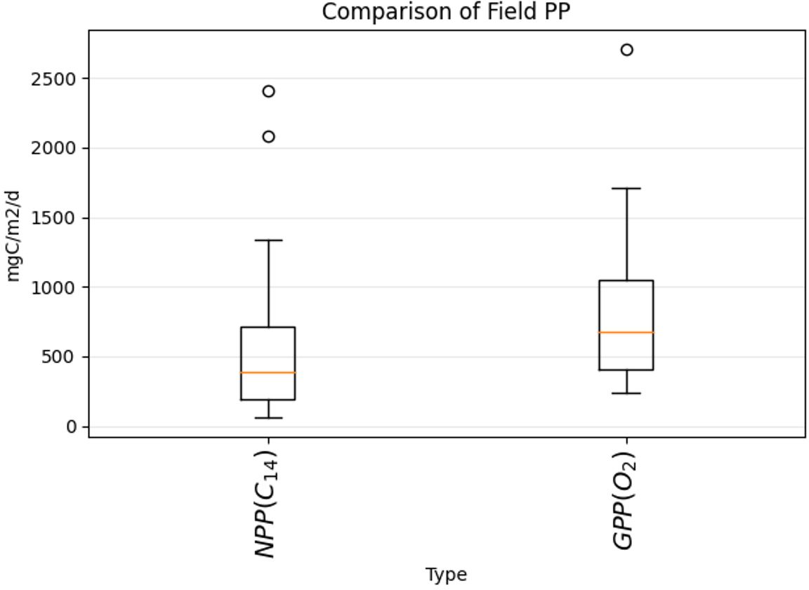
Figure 6. Comparison of values range for field NPP measured with ¹⁴C method (left bar, historical data, see Section 2.3.3.1 for details) and our GPP measured with dissolved O₂ evolution (right bar, see Section 2.3.2 for details). The red lines indicate the median values.

The fact that our GPP_O2 values in general are not as high as expected could come from the difference in the integration depth between the two methods. All the GPP_O2 data were integrated up to 25 m, while the NPP_C14 data have different integration depths, varying from 30 m to 60 m. Unfortunately, it was not possible to have the same integration depths for both methods, as the majority of the ¹⁴C data from the literature had only integrated values. To sum up, the results show that similar spatial patterns for PP are obtained for the two datasets accomplished with different PP methods, collected in different years and seasons. The standard deviation of the triplicate measurements that were then converted to GPP was 38 mgC/m³/day for the difference between the first and last light bottle measurements, and 50 mgC/m³/day for the difference between the first and last dark bottle measurements.

3.2 Sensitivity study

To test satellite-based PP model sensitivity to changes in different model configurations, we have assessed which parameter affected the model output most. For this, we have calculated the RMSD difference between matchups of field PP and modelled PP within each of the groups of tested parameters as listed in Section 2.4. For groups assessing the source and the vertical distribution of CHL data, the difference was the least. The minimum was observed for group 1, the source of CHL data, with a difference in RMSD of 0.001, and for group 3, difference in the shape of a CHL profile, the difference in RMSD was also low 0.011. Group 5, the difference in integration depth, showed also quite a low RMSD difference of 0.032. The largest RMSD difference was observed for the groups assessing the light field - group 2, source of PAR data, showed a 0.254 difference, and group 4, choice of PAR or PUR spectra, showed a 0.195 difference.

This result is contradictory to most of the PP model sensitivity studies, where differences in CHL data generally have more influence on the final output than PAR data (e.g. Carr et al., 2006; Lee et al., 2015; Saba et al., 2011). This could be explained by the fact that in this study the CHL data differ only in processing algorithms, while the PAR data differ in both processing algorithms and sensors. Here, as for our current knowledge, take for the first time Level 2 PAR data from Eumetsat for PP modelling, which has larger values than Glocolour PAR Level 3 data. The difference within group 4, i.e. choosing the PAR spectrum, as in the simplified version of Morel (1991), or the PUR spectrum, as in the full version of Antoine and Morel (1996), is basically a choice between two physically different models, which explains a large difference.

3.3 Choice of the best-performing model setup

We have analysed the matchups for six different versions of in situ data set: three non-interpolated versions, 1) NPP_C14 dataset, 2) GPP_O2 dataset, and 3) NPP_C14 together with GPP_O2 data set. To get the same number of collocations for all the models, we have alternatively spatially interpolated primary production model setups with CHL L3 fields in them to have the same valid data points as in model setups with CHL L4 fields (if the modelled PP data was missing, it was interpolated using the method described in the first paragraph of Section 2.5). This resulted in three other cases: 4) interpolated NPP_C14 dataset, 5) interpolated GPP_O2 dataset, and 6) interpolated NPP_C14 together with GPP_O2 dataset.

For a general overview of the differences in model setups we first show the single bar plot with all the model versions for just one of the datasets that has maximum number of field points for all the combinations (41 points) interpolated NPP_C14+GPP_O2 dataset (Figure 7; Table 2). In Table 2 it is clear that the interpolated datasets do not always reach the maximum number of available data points, for example, 45 available points for NPP_C14+GPP_O2 dataset give only 41 matchups in its interpolated version. In the interpolated dataset, our goal was to obtain an equal number of collocations for all the model setups. Points that were not interpolated as they were outlying the area with available data were excluded. Points that were not present in Copernicus-GlobColour L4 PP data based on Antoine and Morel (1996) were also excluded.

Figure 7

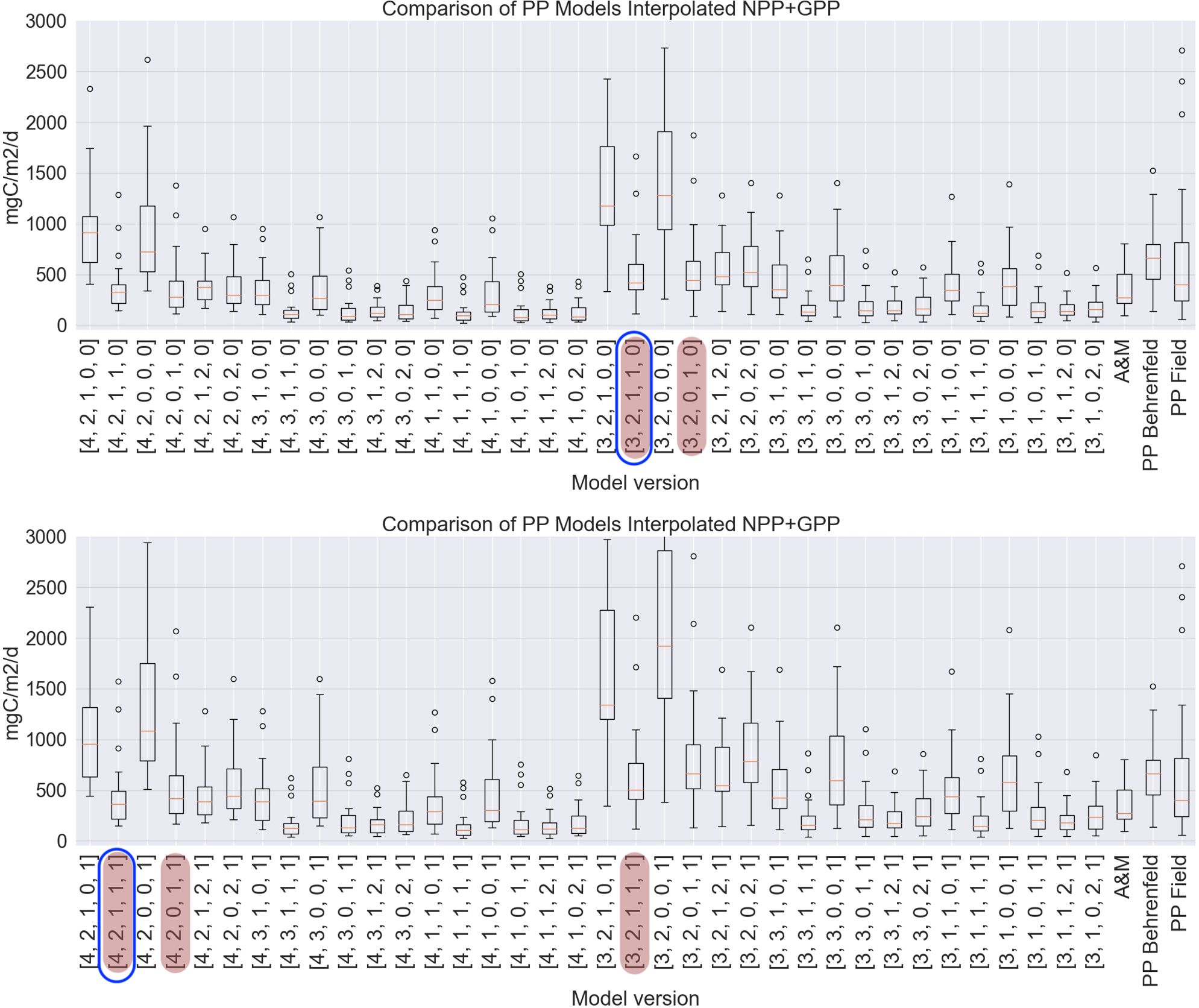
Figure 7. Bar plots illustrating the range of PP values for each model setup for 41 field points of both NPP_C14 and GPP_O2 with spatially interpolated chlorophyll data. Red line: median, bubbles: outliers, box: interquartile range. Top: model versions integrated to the euphotic layer depth, bottom: model versions integrated to the productive layer depth. Model versions have identification number [a,b,c,d,e]; [a]: 3 - Level 3 CHL, 4 - Level 4 CHL; [b]: 1 - Reanalysis PAR, 2 - Level 2 PAR, 3 - Level 3 PAR; [c]: 0 - Global CHL profile, 1 - Local CHL profile; [d]: 0 - no coefficient applied to PAR, 1 - PAR converted to local PUR, 2 - PAR converted to global PUR; [e]: 0 - profiles integrated till euphotic layer depth, 1 - profiles integrated till productive layer depth. Model versions reproducing field data best in terms of bias and correlation coefficient are highlighted (see Section 2.5), two models selected for further calculations are additionally outlined in blue. ‘A&M’ refers to Copernicus-GlobColour L4 PP data based on Antoine and Morel (1996). ‘PP Behrenfeld’ refers to our own calculations of PP based on Behrenfeld(1998) and Globcolour L3 CHL. The last bar corresponds to in situ primary production.

Table 2

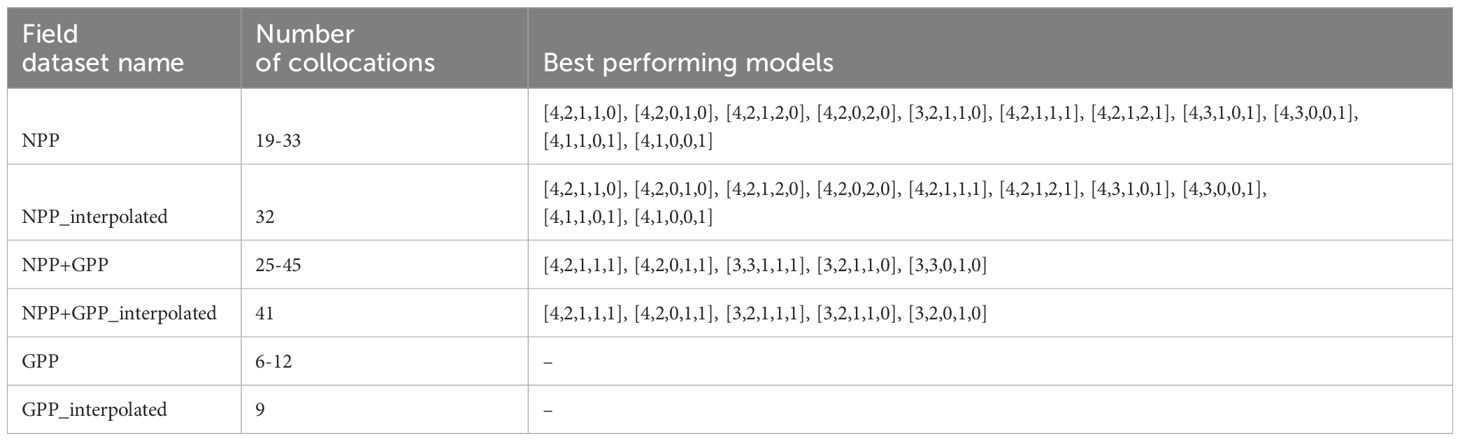
Table 2. Name of field datasets with the selection of best performing models in terms of bias and correlation coefficient (see Section 2.5).

Models selected as a result of this chapter passed the two criteria performance test: (1) bias was close to 0 (-0.1<bias<0.1), and (2) Pearson’s correlation coefficient (r) was greater than the model average (0.25), and are highlighted in blue; details will follow below.

Now we present all six versions of the field dataset, and how they passed the performance test described in the last paragraph in Section 2.5. In the case of the NPP_C14 datasets, many models passed the performance test and were able to reproduce the field data. These were ten combinations in the case of an interpolated dataset, and eleven combinations in the case of the noninterpolated dataset. In the case of the GPP_O2 data set with 12 points, no model combinations passed the performance test for the bias criteria (it was larger than +/-0.1), while correlation coefficients passed the criteria (larger than 0.25). This could be either due to a small number of points or because of the larger values of PP in this dataset. For the NPP_C14+GPP_O2 dataset, five combinations performed well for both interpolated and noninterpolated cases (see Table 2).

For NPP_C14 datasets, model setups with L4 CHL performed better than those with L3 CHL. For NPP_C14+GPP_O2 datasets, the best performing versions always had L2 PAR and local absorption spectrum.

For further calculations we’ve chosen the model versions that passed the performance test to reproduce both the NPP_C14 dataset and the NPP_C14+GPP_O2 dataset. These were the two versions: [4,2,1,1,1] and [3,2,1,1,0], see the blue highlight in Figure 7. P-value of correlation was significant for both model versions (p<0.05). Both of the versions contain Level 2 PAR, local CHL-a profile, and local absorption spectrum. In terms of values, one can see that both of these models have a range of values similar to field data in combination with several high outliers (Figure 7).

Similar patterns are clear in the target diagrams, which have slightly different metrics and thus give results that are not identical to a performance test (Figure 8). The target diagram uses uRMSD and relative bias, as opposed to a performance test that uses the correlation coefficient and bias. The closer the model is to the target, the better the model performs. One can see that for NPP_C14+GPP_O2 interpolated dataset (41 points), the same five models as previously mentioned are performing best, and three more models with CHL L4, PAR L2, and local CHL profile were added to them. For NPP_C14 interpolated dataset (32 points) the patterns are also similar to performance test, with the majority of well-performing models using CHL L4. It is also worth noting that the global Antoine and Morel model also performs quite well according to these metrics, but not reaching the inner part of the circle as other model setups.

Figure 8

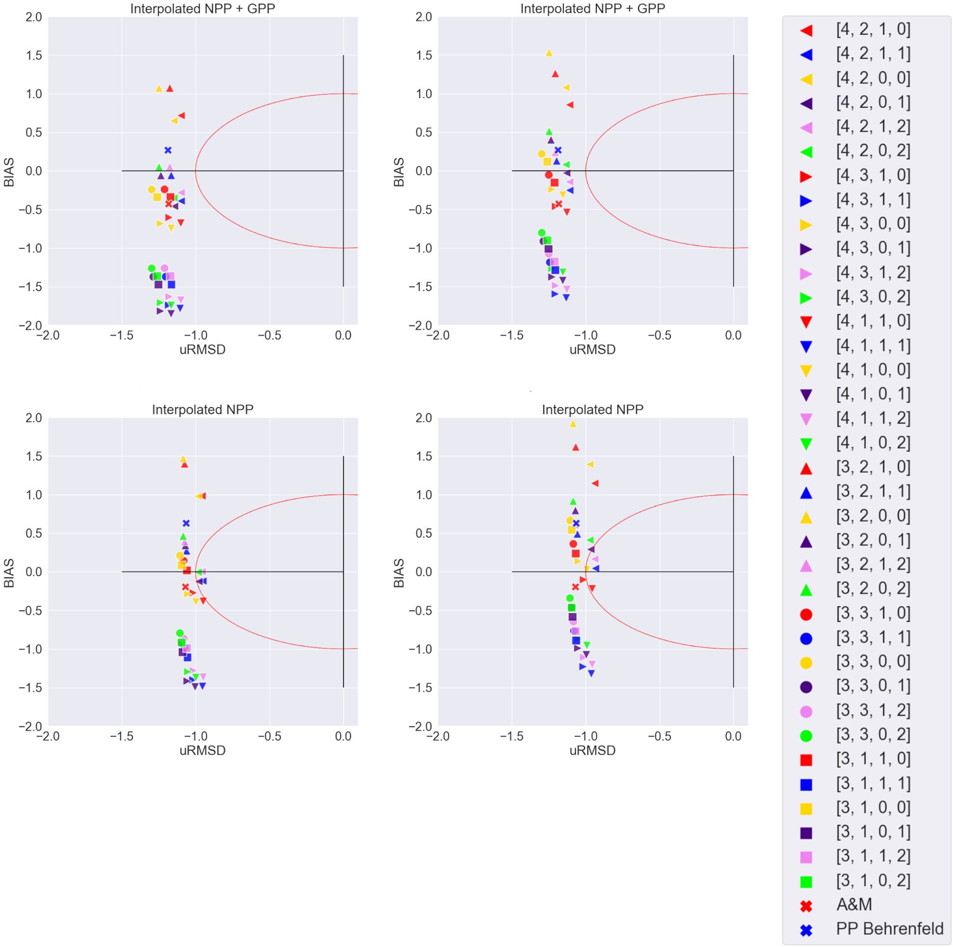
Figure 8. Target diagrams illustrating relative model performance in reproducing field PP data. Right half of the diagrams is cut due to a lack of data in that area. The red circle is the normalized standard deviation of the in situ PP data. Top: NPP_C14+GPP_O2 interpolated dataset; bottom: NPP_C14 interpolated dataset; left: vertical profiles integrated to the depth of the euphotic layer; right: vertical profiles integrated to the depth of the productive layer. Legend has model identification number [a,b,c,d]; [a]: 3 - Level 3 CHL, 4 - Level 4 CHL; [b]: 1 - Reanalysis PAR, 2 - Level 2 PAR, 3 - Level 3 PAR; [c]: 0 - Global CHL profile, 1 - Local CHL profile;[d]: 0 - no coefficient applied to PAR, 1 - PAR converted to local PUR, 2 - PAR converted to global PUR; ‘A&M’ refers to Copernicus-GlobColour L4 PP data based on Antoine and Morel (1996). ‘PP Behrenfeld’ refers to our own calculations of PP based on Behrenfeld (1998) and Globcolour L3 CHL. This Figure has four groups instead of five used previously as here the fifth group is differentiated using left and right sides of the Figure not to overload each of the diagrams with symbols.

The choice of different PQ values did not significantly affect the results, no changes in the selected best-performing models were made when using 1.4 instead of 1.25, and one additional model [4,3,0,0,1] with a higher range of values passed the performance test when using the PQ value of 1.0 instead of 1.25.

As a result of this section, for further calculations we’ve chosen the two model versions that passed the performance test best. These two versions are also close to the target in Figure 8: [4,2,1,1,1] - blue east-oriented triangle on right images, and [3,2,1,1,0] - blue north-oriented triangle on left images, giving similar results of choosing the best model using different methods. Figure 8 denotes four groups instead of five groups the fifth group it is differentiated using the left and right sides of the Figure not to overload each of the separate diagrams with symbols. Model setup [4,2,1,1,1] uses Copernicus-GlobColour Level 4 CHL, EUMETSAT Level 2 OLCI PAR, the local CHL profile following Cherkasheva et al. (2013), PAR converted to local PUR, and profiles integrated till productive layer depth. The setup [3,2,1,1,0] uses Globcolour Level 3 CHL, EUMETSAT Level 2 OLCI PAR, local CHL profile following Cherkasheva et al. (2013); PAR converted to local PUR and profiles integrated till euphotic layer.

3.4 Basin estimates and trends

For the two models selected in the previous section, we calculated the basin primary production estimates for the two regions plotted in Figure 4 for our results to be comparable with Hill et al. (2013) estimates (red region) and Arrigo and van Dijken (2015) estimates (blue region).

The monthly basin estimates were present only in Hill et al. (2013) paper, and are shown corrected by us for the SCM presence using the method applied by Hill et al. (2013). Annual Hill et al. (2013) estimates account for SCM and did not have to be corrected.

The results of the basin estimates for the two models selected in our study are presented in Table 3. We have tested calculations with both interpolating the missing pixels of data and not, but there was only a 0.5 TgC/year (less than 1%) difference between the two models selected in our study. Thus, here we show the noninterpolated values. The difference between the estimates of the two models on average was minor, about 1-4% of the annual estimates for 1998-2022 depending on the choice of the region. The annual average was 342-347 TgC/year. The results are slightly higher than Hill et al. (2013) results, which give 308 TgC/year. This difference could be attributed to the principal differences between the models used. Hill et al. (2013) calculations are based on a model developed for the Chukchi Sea, which uses SeaWiFS CHL data only, without accounting for PAR data (Hill and Zimmerman, 2010). In our case, CHL data are an integrated product of several sensors, PAR data is used, and the model includes Greenland Sea parameterizations derived from particulate absorption and CHL data. Our model results calculated for the basin grid used in Arrigo and van Dijken (2015), were with an annual average of 340 TgC/year annual average significantly higher than the 136.3 TgC/year reported in that study. These results are difficult to compare as Arrigo and van Dijken (2015) did not yet account for the SCM, which has a potentially increasing impact on integrated primary production in the Arctic with time (Ardyna and Arrigo, 2020). Previously we have estimated that the omission of SCM in Antoine and Morel (1996) primary production model resulted on average in 10% underestimation of the PP for the Greenland Sea (Cherkasheva et al., 2013), while studies for different models suggest a larger impact (Ardyna et al., 2013; Hill et al., 2013). In terms of a seasonal evolution, our results are more uniform throughout the year, ranging between 33 TgC/month to 78 TgC/month, while Hill et al. (2013) estimates show a wider range of 13-123 TgC/month. This seasonal dynamics that we have observed is in line with the pattern that we have previously seen when analysing CHL data in the area (Nöthig et al., 2015). In our models, the peak of the bloom is observed in May for the Nordic Seas region similar to Hill et al. (2013). For the larger and further north region of Arrigo and van Dijken (2015), the peak value shifts to June, though the values in May are close as well. The spatial distribution of this bloom is seen in the monthly maps (Figure 9). When compared to Ardyna et al. (2013) 228-230 TgC/year estimates, our results as in all other cases give higher regional PP estimates of 333 TgC/year. This could be due to the fact that ten validation points for the region used in Ardyna et al. (2013) are distributed in the Western part of the Greenland Sea which is less productive than the Eastern part. The data set on which we based the selection of the model setup is, on the other hand, distributed in both the western and eastern parts of the Greenland Sea (Figure 5). The other reason could be the different parametrizations of the CHL vertical profile. In general, our larger estimates than those previously reported could have been explained by our additional use of GPP field data which has higher values than NPP. However, as we have tested, the selected models are best at reproducing NPP data without GPP data as well (Section 3.3). Another point worth noting is that although mentioned studies (Ardyna et al. (2013); Arrigo and van Dijken (2011); Hill et al. (2013)) accurately use local data from the Greenland Sea, in principle they are pan-Arctic studies and have less Greenland Sea parametrization parameters than used here.

Table 3

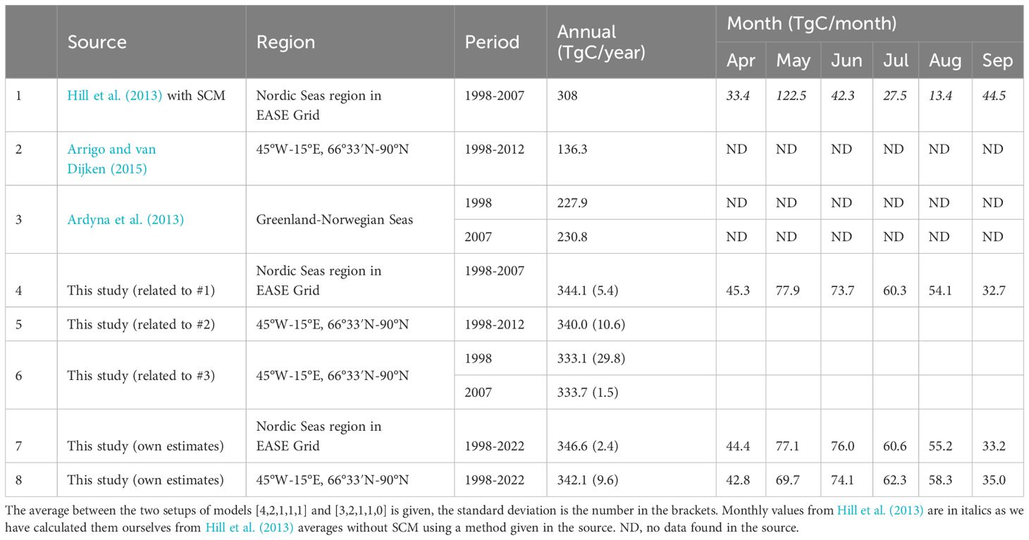
Table 3. Primary production basin estimates in the European Arctic from literature and calculated in this study using two models selected via performance tests in Section 3.3.

Figure 9

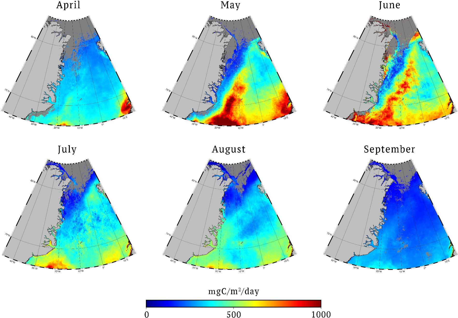
Figure 9. Monthly primary production for 1998-2022 for one of the selected model setups [4,2,1,1,1], which uses Copernicus-GlobColour Level 4 CHL, EUMETSAT Level 2 OLCI PAR, local CHL profile following Cherkasheva et al. (2013), PAR converted to local PUR and profiles integrated till productive layer depth.

When looking at the trends for the selected regions, no significant increase or decrease in primary production was found in the period 1998-2022 (see Figure 10). Spatial standard deviation for the monthly values on Figure 10 ranged from 18 to 92 mgC/m²/day.

Figure 10

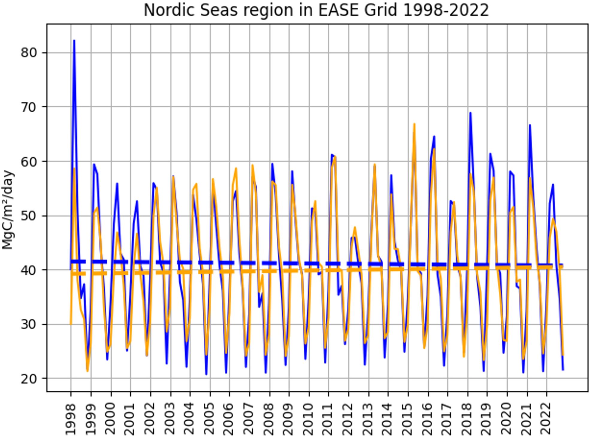
Figure 10. Time series and trend line for one of the two selected primary production model setups and the Nordic Seas region in the EASE grid for 1998-2022. Orange line: model setup [3,2,1,1,0], blue line: model setup [4,2,1,1,1]. The trends are significant (p<0.01).

4 Discussion

4.1 Field estimates

Although GPP measurements with oxygen sensors are not traditional, in our case they gave estimates comparable to historical NPP values derived with the ¹⁴C method for the Greenland Sea in terms of spatial patterns and 1.5 higher estimates in terms of average values. Range of GPP values was higher than for NPP, as GPP does not account for AR (Eq. 3).

The method should be applied with care, as the sensors are very sensitive to temperature changes and the way sampling bottles are filled, so an error could easily be introduced. We also recommend having triplicate samples for each measurement to minimise errors. The average standard deviation of triplicate measurements was 38-50 mgC/m³/day for the difference between the initial and the last measurements. Unfortunately, we did not have simultaneous measurements of primary production with the other methods to be able to perform a direct intercomparison. In summary, we would recommend using oxygen sensors in a setup presented here to get a rough estimate of GPP, especially as an alternative in case of absence of ¹⁴C and ¹³C measurements of NPP, which are accordingly legally and logistically challenging.

4.2 Choice and performance of the model

According to the study by Lee et al. (2015) of the Arctic PP models, depth-resolved CHL models agreed better with in-situ data than any other type. This was a decisive factor for us in choosing a depth-resolved CHL model to work with. However, Lee et al. (2015) also mention that absorption-based models as well do have potential, since they exhibit lowest bias associated with weaker correlation when compared to field PP. Antoine et al. (2013) give a similar point of view recommending to use either locally tuned CHL algorithms for the Arctic, or not-CHL based algorithms (e.g., Hirawake et al., 2012; Mouw and Yoder, 2005). According to Antoine et al. (2013), combining the retrieval of nonwater absorption with locally tuned models for CDOM absorption (Matsuoka et al., 2013), might improve absorption-based models. Thus, the next step to achieve a goal of more accurate Greenland Sea PP estimates could be to test the absorption models focused precisely on the Greenland Sea and not on the Arctic as a whole, as previously done in Lee et al. (2015).

Our result clearly and expectedly showed that model setups with local CHL profile and local absorption spectrum perform better than global relationships. The fact that level 2 PAR is performing better than level 3 PAR is more challenging to explain. This could just be a mathematical feature of level 2 PAR having larger values, and thus these models follow closer the range of in-situ data. For the Arctic study by Lee et al. (2015), the best-performing cases were the models that used in situ CHL and satellite PAR, but they did not test PAR data from different sensors, and no conclusions could be made between the performance of L2 and L3 PAR.

The accuracy of the model ability here to reproduce the field data in terms of RMSD is poorer than reported for the global studies: the average RMSD for our selected model setups is 0.4 as opposed to RMSD=0.3 reported as an average for 21 models by Saba et al. (2011) tested in ten marine regions across the world. For the Arctic, however, the performance of our selected model setups is much better than the average shown in the Arctic intercomparison study by Lee et al. (2015), where the RMSD range is 0.61-0.67 for 32 models, and averages 0.65 for the depth resolved models as those used in this study.

5 Conclusion

We have collected an integrated field dataset of net primary production data obtained with the ¹⁴C method (NPP_C14), and gross primary production obtained with optode O₂ measurements (GPP_O2). Various setups of a commonly used primary production model were tested incorporating n both local and global empirical relationships and input data from diverse sources. The model versions that performed best when validated against the NPP_C14 and GPP_O2 data included the local CHL profile and local absorption spectrum in their setup and used the Level 2 PAR data as input. In terms of the choice of CHL input data and integration depth, there was no dependency.

Our basin-wide estimates for the Nordic Seas exceed those of previous studies, averaging 347 TgC/year for 1998–2022 — 11% higher than one prior estimate and 150% higher than another. The seasonal cycle in our case has less monthly variation of 33-78 TgC/month than 13-123 TgC/month previously reported with the peak production similarly observed in May, and no significant trends in primary production was observed when studying regionally averaged estimates.

The accuracy of the selected model setups to reproduce the field data in terms of RMSD is poorer than in the related global studies, but better than in the related Arctic studies. Using absorption-based models, especially in CDOM-dominated areas such as western part of the Greenland Sea may improve the quality of primary production estimates and could be a next step toward improving primary production estimates in the Greenland Sea.

The primary production estimates obtained here, along with the algorithm, are valuable for biogeochemical studies in the area, particularly in assessing carbon dioxide uptake by phytoplankton and carbon flux. The insights gained from the algorithm’s development, including the factors that improved its performance, offer useful guidance for enhancing other regional primary production models.

Data availability statement

Primary production measured with optode O₂ measurements for 2021-2022 has been uploaded to PANGAEA Data Publisher for Earth & Environmental Science, https://doi.pangaea.de/10.1594/PANGAEA.965985. The Python codes developed for this manuscript are available at https://github.com/9Di/environmental_data_algorithms/tree/main/Algorithms.

Author contributions

AC: Conceptualization, Data curation, Formal analysis, Funding acquisition, Investigation, Methodology, Project administration, Resources, Supervision, Validation, Visualization, Writing – original draft, Writing – review & editing. RM: Data curation, Formal analysis, Software, Writing – review & editing. PK: Conceptualization, Funding acquisition, Investigation, Project administration, Resources, Supervision, Writing – review & editing. AL: Conceptualization, Validation, Writing – review & editing. MZ: Investigation, Writing – review & editing. AB: Conceptualization, Supervision, Writing – review & editing.

Funding

The author(s) declare financial support was received for the research, authorship, and/or publication of this article. The research leading to these results has received funding from the Norwegian Financial Mechanism 2014-2021, NCN-POLS project MOPAR no. 2020/37/K/ST10/03254 awarded to Dr. Aleksandra Cherkasheva, and it was in addition partially supported by a the National Science Centre of the Republic of Poland (NCN), through OPUS26 project OptiCal-Green, contract no. UMO-2023/51/B/ST10/01344, awarded to Prof. Piotr Kowalczuk. The authors used datasets collected during the CDOM-HEAT project (2013-2016) supported by the Polish‐Norwegian Research Programme operated by the National Centre for Research and Development under the Norwegian Financial Mechanism 2009–2014 in the framework of the project contract Pol–Nor/197511/40/2013. Dr. Aleksandra Cherkasheva’s contribution was supported by Norwegian Financial Mechanism 2014-2021, NCN-POLS project MOPAR no. 2020/37/K/ST10/03254 and by the European Union’s Horizon Europe Research and Innovation programme under Grant Agreement No. 101136748 (BioEcoOcean). Prof. Piotr Kowalczuk’s participation in the Maria S. Merian 2022 expedition was supported by the European Union's Horizon 2020 research and innovation programme under grant agreement No. 869383 (ECOTIP). Prof. Astrid Bracher’s contribution was supported in part by Helmholtz Impulse Fond DFG (German Research Foundation) Transregional Collaborative Research Centre ArctiC Amplication: Climate Relevant Atmospheric and SurfaCe Processes, and Feedback Mechanisms (AC)3 (Project C03) and by the Helmholtz Infrastructure Initiative FRAM. The contribution of Dr. Alexandra Loginova was supported by Norwegian Financial Mechanism 2014-2021: DOMUSe (2020/37/K/ST10/03018) and by the Polish National Sciences Center NCN SONATA BIS-9 Call grant no. 2019/34/E/ST10/00167 under the project PROSPECTOR. The contribution of Dr. Monika Zabłocka was supported by the National Science Centre within the framework of project DOMinEA contract no. UMO-2021/41/ B/ST10/03603. The draft idea of the current study was developed in 2013 and supported at that time by POLMAR Helmholtz Graduate School for Polar and Marine research and Helmholtz Impulse and Network Fond at the Alfred-Wegener-Institute (project PHYTOOPTICS) contributing to the long term ecological observations in Fram Strait (PACES program). The ship-time on board RV Kronprins Haakon during the FS2021 cruise leading to the results of this study was funded by the European Union H2020 as part of the EU Project ARICE grant agreement No. 730965.

Acknowledgments

We thank Dr. Vasiliy Povazhnyy for the training on measuring GPP with oxygen sensors and consultations when preparing for the cruise and processing the data, and Dr. Elena Terzic for the help in field measurements onboard RV Maria S. Merian August 2022 cruise. We acknowledge the contribution of Zofia Smoła and Wiktor Józef in obtaining historical NPP measurements. Dr. Aleksandra Cherkasheva thanks Prof. David Antoine and Bernard Gentili for the instructions on the Morel (1991) model setup which she received during her PhD work. The authors also thank the entire crews of RV Kronprins Haakon and RV Maria S. Merian for their time and effort, and acknowledge satellite data and reanalysis data providers (NOAA/NCEP, Copernicus Marine Service, EUMETSAT, ACRI-ST) for developing and distributing the data.

Conflict of interest

The authors declare that the research was conducted in the absence of any commercial or financial relationships that could be construed as a potential conflict of interest.

The author(s) declared that they were an editorial board member of Frontiers, at the time of submission. This had no impact on the peer review process and the final decision.

Publisher’s note

All claims expressed in this article are solely those of the authors and do not necessarily represent those of their affiliated organizations, or those of the publisher, the editors and the reviewers. Any product that may be evaluated in this article, or claim that may be made by its manufacturer, is not guaranteed or endorsed by the publisher.

References

Alexander V., Niebauer H. J. (1981). Oceanography of the eastern Bering Sea ice-edge zone in spring, Limnol. Oceanography 26, 1111–1125. doi: 10.4319/lo.1981.26.6.1111

Crossref Full Text | Google Scholar

Antoine D., André J.-M., Morel A. (1996). Oceanic primary production: 2. Estimation at global scale from satellite (Coastal Zone Color Scanner) chlorophyll. Global Biogeochemical Cycles 10, 57–69. doi: 10.1029/95GB02832

Crossref Full Text | Google Scholar

Antoine D., Hooker S. B., Bélanger S., Matsuoka A., Babin M. (2013). Apparent optical properties of the Canadian Beaufort Sea – Part 1: Observational overview and water column relationships. Biogeosciences 10, 4493–4509. doi: 10.5194/bg-51310-4493-2013

Crossref Full Text | Google Scholar

Antoine D., Morel A. (1996). Oceanic primary production: 1. Adaptation of a spectral light-photosynthesis model in view of application to satellite chlorophyll observations. Global Biogeochemical Cycles. 10, 43–55. doi: 10.1029/95GB02831

Crossref Full Text | Google Scholar

Ardyna M., Arrigo K. R. (2020). Phytoplankton dynamics in a changing Arctic Ocean. Nat. Climate Change 10, 892–903. doi: 10.1038/s41558-020-0905-y

Crossref Full Text | Google Scholar

Ardyna M., Babin M., Gosselin M., Devred E., Belanger S., Matsuoka A., et al. (2013). Parameterization of vertical chlorophyll a in the Arctic Ocean: Impact of the subsurface chlorophyll maximum on regional, seasonal, and annual primary production estimates. Biogeosciences 10, 4383–4404. doi: 10.5194/bg-10-4383-2013

Crossref Full Text | Google Scholar

Ardyna M., Mundy C. J., Mayot N., Matthes L. C., Oziel L., Horvat C., et al. (2020). Under-ice phytoplankton blooms: shedding light on the “Invisible“ Part of arctic primary production. Front. Mar. Sci. 7. doi: 10.3389/fmars.2020.608032

Crossref Full Text | Google Scholar

Arrigo K. R., van Dijken G. L. (2011). Secular trends in Arctic Ocean net primary production. J. Geophysical Res. 16. doi: 10.1029/2011JC7273C09011

Crossref Full Text | Google Scholar

Arrigo K. R., van Dijken G. L. (2015). Continued increases in Arctic Ocean primary production. Prog. Oceanography 136, 60–70. doi: 10.1016/j.pocean.2015.05.002

Crossref Full Text | Google Scholar

Assmy P., Fernández-Méndez M., Duarte P., Meyer A., Randelhoff A., Mundy C. J., et al. (2017). Leads in Arctic pack ice enable early phytoplankton blooms below snow-covered sea ice. Sci. Rep. 7, 40850. doi: 10.1038/srep40850

PubMed Abstract | Crossref Full Text | Google Scholar

Balch W. M., Carranza M., Cetinić I., Chaves J. E., Duhamel S., Fassbender A., et al. (2022). “IOCCG protocol series: aquatic primary productivity field protocols for satellite validation and model synthesis,” in IOCCG ocean optics and biogeochemistry protocols for satellite ocean colour sensor validation, 7.0. Eds. Vandermeulen R. A., Chaves J. E. (Dartmouth, NS, Canada: International Ocean Colour Coordinating Group (IOCCG)). doi: 10.25607/OBP-1835

Crossref Full Text | Google Scholar

Bashmachnikov I. L., Fedorov A. M., Golubkin P. A., Vesman A. V., Selyuzhenok V. V., Gnatiuk N. V., et al. (2021). Mechanisms of interannual variability of deep convection in the Greenland Sea. Deep Sea Res. Part I: Oceanographic Res. Papers 174, 103557. doi: 10.1016/j.dsr.2021.103557

Crossref Full Text | Google Scholar

Behrenfeld M. J., Falkowski P. G. (1997). Photosynthetic rates derived from satellite-based chlorophyll concentration. Limnology Oceanography 42, 1–20. doi: 10.4319/lo.1997.42.1.0001

Crossref Full Text | Google Scholar

Behrenfeld M. J., Prasil O., Kolber Z. S., Babin M., Falkowski P.G. (1998). Compensatory changes in photosystem II electron turnover rates protect photosynthesis from photoinhibition. Photosynth. Res., 58, 259–268.ll concentration. Limnology Oceanography. 42, 1–20. doi: 10.1023/A:1006138630573

Crossref Full Text | Google Scholar

Bélanger S., Babin M., Tremblay J.-E. (2013). Increasing cloudiness in the Arctic damps the increase in phytoplankton primary production due to sea ice receding. Biogeosciences 10, 4087–4101. doi: 10.5194/bg-10-4087-2013

Crossref Full Text | Google Scholar

Boyer Tim P., Garcia Hernan E., Locarnini Ricardo A., Zweng Melissa M., Mishonov Alexey V., Reagan James R., et al. (2018). World Ocean Atlas 2018. [Statistical mean of Mixed Layer Depth on 1° grid for all decades] (NOAA National Centers for Environmental Information. Dataset). Available online at: https://www.ncei.noaa.gov/archive/accession/NCEI-WOA18 (Accessed 17.01.2023).

Google Scholar

Bricaud A., Babin M., Morel A., Claustre H. (1995). Variability in chlorophyll-specific absorption coefficients of natural phytoplankton: Analysis and parameterization. J. Geophysical Res. 100, 13,321–13,332. doi: 10.1029/95JC00463

Crossref Full Text | Google Scholar

Campbell K., Mundy C. J., Landy J. C., Delaforge A., Michel C., Rysgaard S. (2016). Community dynamics of bottom-ice algae in Dease Strait of the Canadian Arctic. Prog. Oceanography 149, 27–39. doi: 10.1016/j.pocean.2016.10.005

Crossref Full Text | Google Scholar

Carpenter J. (1995). The accuracy of the winkler method for dissolved oxygen analysis (Baltimore, MD: The Johns Hopkins University), 135–140.

Google Scholar

Carr M. E., Friedrichs M. A., Schmeltz M., Aita M. N., Antoine D., Arrigo K. R., et al. (2006). A comparison of global estimates of marine primary production from ocean color. Deep-Sea Res. Part II: Topical Stud. Oceanography 53, 741–770. doi: 10.1016/j.dsr2.2006.01.028

Crossref Full Text | Google Scholar

Carritt D. E., Carpenter J. H. (1966). Comparison and evaluation of currently employed modifications of the Winkler method for determining dissolved oxygen in seawater; A NASCO report. J. Mar. Res. 24. Available online at: https://elischolar.library.yale.edu/journal_of_marine_research/1077.

Google Scholar

Chassot E., Bonhommeau S., Dulvy N. K., Mélin F., Watson R., Gascuel D., et al. (2010). Global marine primary production constrains fisheries catches. Ecol. Lett. 13, 495–505. doi: 10.1111/j.1461-0248.2010.01443.x

PubMed Abstract | Crossref Full Text | Google Scholar

Cherkasheva A., Nöthig E.-M., Bauerfeind E., Melsheimer C., Bracher A. (2013). From the chlorophyll a in the surface layer to its vertical profile: a Greenland Sea relationship for satellite applications. Ocean Sci. 9, 431–445. doi: 10.5194/os-9-431-2013

Crossref Full Text | Google Scholar

Cherkasheva A., Bracher A., Melsheimer C., Koberle C., Gerdes R., Nothig E.­ M., et al. (2014). Influence of the physical environment on polar phytoplankton blooms: a case study in the Fram Strait. J. Mar. Syst. 132, 196­–207. doi: 10.1016/j.jmarsys.2013.11.008

Crossref Full Text | Google Scholar

Chierici M., Vernet M., Fransson A., Børsheim K. Y. (2019). Net community production and carbon exchange from winter to summer in the atlantic water inflow to the arctic ocean. Front. Mar. Sci. 6. doi: 10.3389/fmars.2019.00528

Crossref Full Text | Google Scholar

Cota G. F., Wang J., Comiso J. C. (2004). Transformation of global satellite chlorophyll retrievals with a regionally tuned algorithm. Remote Sens. Environ. 90, 373–377. doi: 10.1016/j.rse.2004.01.005

Crossref Full Text | Google Scholar

Duarte C. M., Agustí S. (1998). The CO2 balance of unproductive aquatic ecosystems. Science 281, 234–236. doi: 10.1126/science.281.5374.234

PubMed Abstract | Crossref Full Text | Google Scholar

Duarte C. M., Agustí S., Regaudie-de-Gioux A. (2011). “The role of marine biota in the metabolism of the biosphere,” in The role of marine biota in the functioning of the biosphere. Ed. Duarte C. M. (CSIC, Madrid), 38–53.

Google Scholar

Eastman R., Warren S. G. (2010). Interannual variations of Arctic cloud types in relation to sea ice. J. Climate 23, 4216–4232. doi: 10.1175/2010JCLI3492.1

Crossref Full Text | Google Scholar

Gonçalves-Araujo R., Granskog M. A., Bracher A., Azetsu-Scott K., Dodd P. A., Stedmon C. A. (2016). Using fluorescent dissolved organic matter to trace and distinguish the origin of Arctic surface waters. Sci. Rep. 6. doi: 10.1038/srep33978

PubMed Abstract | Crossref Full Text | Google Scholar

Granskog M. A., Stedmon C. A., Dodd P. A., Amon R. M. W., Pavlov A. K., de Steur L., et al. (2012). Characteristics of colored dissolved organic matter (CDOM) in the Arctic outflow in the Fram Strait: Assessing the changes and fate of terrigenous CDOM in the Arctic Ocean. J. Geophys. Res. 117, C12021. doi: 10.1029/2012JC008075

Crossref Full Text | Google Scholar

Hansell D. A., Carlson C. A., Repeta D. J., Schlitzer R. (2009). Dissolved organic matter in the ocean: A controversy stimulates new insights. Oceanography 22, 202–211. doi: 10.5670/oceanog.2009.109

Crossref Full Text | Google Scholar

Hill V. J., Matrai P. A., Olson E., Suttles S., Steele M., Codispoti L. A., et al. (2013). Synthesis of integrated primary production in the Arctic Ocean: II. In situ and remotely sensed estimates. Prog. Oceanography 110, 107–125. doi: 10.1016/j.pocean.2012.11.005

Crossref Full Text | Google Scholar

Hill V. J., Zimmerman R. C. (2010). Assessing the accuracy of remotely sensed primary production estimates for the Arctic Ocean, using passive and active sensors. Deep Sea Res. I 57, 1243–1254. doi: 10.1016/j.dsr.2010.06.011

Crossref Full Text | Google Scholar

Hirawake T., Shinmyo K., Fujiwara A., Saitoh S. I. (2012). Satellite remote sensing of primary productivity in the Bering and Chukchi Seas using an absorption-based approach. ICES J. Mar. Sci. 69, 1194–1204. doi: 10.1093/icesjms/fss111

Crossref Full Text | Google Scholar

Intrieri J., Fairall C. W., Shupe M. D., Persson P. O. G., Andreas E. L., Guest P. S., et al. (2002). An annual cycle of Arctic surface cloud forcing at SHEBA. J. Geophysical Res. 107, 8039. doi: 10.1029/2000JC000439

Crossref Full Text | Google Scholar

IOCCG. (2015). “Ocean colour remote sensing in polar seas,” in Dartmouth, NS, Canada, International Ocean-Colour Coordinating Group (IOCCG), eds. Babin M., Arrigo K., Bélanger S., and M-H. Forget (Reports of the International Ocean-Colour Coordinating Group, No. 16), 130. doi: 10.25607/OBP-107

Crossref Full Text | Google Scholar

Iversen K. R., Seuthe L. (2011). Seasonal microbial processes in a high-latitude fjord (Kongsfjorden, Svalbard): I. Heterotrophic bacteria, picoplankton and nanoflagellates. Polar Biol. 34, 731–749. doi: 10.1007/s00300-010-0929-2

Crossref Full Text | Google Scholar

Johannessen J. A., Johannessen O. M., Svendsen E., Schuchman R., Manley T., Cambell W. J., et al. (1987). Mesoscale eddies in the Fram Strait marginal ice zone the 1983 and 1984 Marginal Ice Zone Experiments. J. Geophysical Res. 92, 6754–6772. doi: 10.1029/JC092iC07p06754

Crossref Full Text | Google Scholar

Jolliff J. K., Kindle J. C., Shulman I., Penta B., Friedrichs M. A. M., Helber R., et al. (2009). Summary diagrams for coupled hydrodynamic-ecosystem model skill assessment. J. Mar. Syst. 76, 64–82.

Google Scholar

Kowalczuk P., Sagan S., Makarewicz A., Meler J., Borzycka K., Zabłocka M. (2019). Bio-optical properties of surface waters in the Atlantic Water inflow region off Spitsbergen (Arctic Ocean). J. Geophysical Research: Oceans 124, 1964–1987. doi: 10.1029/2018JC014529

Crossref Full Text | Google Scholar

Kraft A. (2013). Arctic pelagic amphipods - community patterns and life-cycle history in a warming Arctic Ocean. PhD Thesis, FB2 (Germany: University of Bremen).

Google Scholar

Laliberté J., Bélanger S., Frouin R. (2016). Evaluation of satellite-based algorithms to estimate photosynthetically available radiation (PAR) reaching the ocean surface at high northern latitudes. Remote Sens. Environ. 184, 199–211. doi: 10.1016/j.rse.2016.06.014

Crossref Full Text | Google Scholar

Lee Y. J., Matrai P. A., Friedrichs M. A. M., Saba V. S., Antoine D., Ardyna M., et al. (2015). An assessment of phytoplankton primary productivity in the Arctic Ocean from satellite ocean color/in situ chlorophyll-a based models. J. Geophysical Res. Oceans 120, 6508–6541. doi: 10.1002/2015JC011018

PubMed Abstract | Crossref Full Text | Google Scholar

Li Z., Cassar N. (2016). Satellite estimates of net community production based on O2/Ar observations andcomparison to other estimates,GlobalBiogeochem. Cycles 30, 735–752. doi: 10.1002/2015GB005314

Crossref Full Text | Google Scholar

Lorenzen C. L. (1967). Determination of chlorophyll and pheo-pigments: Spectrophotometric equations. Limnology Oceanography 12, 343–346. doi: 10.4319/lo.1967.12.2.0343

Crossref Full Text | Google Scholar

Marker A. F. H., Nusch E. A., Rai H., Riemann B. (1980). The measurement of photosynthetic pigments in freshwaters and standardization of methods: Conclusions and recommendations. Arch. fur Hydrobiologie Beihefte Ergebnisse der Limnologie 14, 91–106.

Google Scholar

Matrai P. A., Olson E., Suttles S., Hill V., Codispoti L. A., Light B., et al. (2013). Synthesis of primary production in the Arctic Ocean: I. Surface waters 1954-2007. Prog. Oceanography 110, 93–106. doi: 10.1016/j.pocean.2012.11.004

Crossref Full Text | Google Scholar

Matsuoka A., Huot Y., Shimada K., Saitoh S., Babin M. (2007). Characteristics of chromophoric and fluorescent dissolved organic matter in the Nordic Seas. J. Remote Sens. 33, 503–518.

Google Scholar

Matsuoka A., Hooker S. B., Bricaud A., Gentili B., Babin M.. (2013). Estimating absorption coefficients of colored dissolved organic matter (CDOM) using a semi-analytical algorithm for southern Beaufort Sea waters: application to deriving concentrations of dissolved organic carbon from space. Biogeosciences 10, 917–927. doi: 10.5194/bg-10-917-2013.

Crossref Full Text | Google Scholar

McLaughlin F. A., Carmack E. C. (2010). Deepening of the nutricline and chlorophyll maximum in the Canada Basin interior 2003-2009. Geophysical Res. Lett. 37, L24602. doi: 10.1029/2010GL045459

Crossref Full Text | Google Scholar

Morel A. (1978). Available, usable, and stored radiant energy in relation to marine photosynthesis. Deep-Sea Res. 25, 673–688. doi: 10.1016/0146-6291(78)90623-9

Crossref Full Text | Google Scholar

Morel A. (1988). Optical modeling of the upper ocean in relation to its biogenous matter content (case I waters). J. Geophysical Res. 93, 10749. doi: 10.1029/jc093ic09p10749

Crossref Full Text | Google Scholar

Morel A. (1991). Light and marine photosynthesis: a spectral model with geochemical and climatological implications. Prog. Oceanography 26, 263–306. doi: 10.1016/0079-6611(91)90004-6

Crossref Full Text | Google Scholar

Morel A., Berthon J. F. (1989). Surface pigments, algal biomass profiles, and potential production of the euphotic layer: relationships reinvestigated in view of remote-sensing applications. Limnology Oceanography 34, 1545–1562. doi: 10.4319/lo.1989.34.8.1545

Crossref Full Text | Google Scholar

Morel A., Maritorena S. (2001). Bio-optical properties of oceanic waters: A reappraisal. J. Geophysical Research: Oceans 106, 7163–7180. doi: 10.1029/2000jc000319

Crossref Full Text | Google Scholar

Mouw C., Yoder J. A. (2005). Primary production calculations in the Mid-Atlantic Bight, including effects of phytoplankton community size structure. Limnology Oceanography 50, 1232–1243. doi: 10.4319/lo.2005.50.4.1232

Crossref Full Text | Google Scholar

Nöthig E.-M., Bracher A., Engel A., Metfies K., Niehoff B., Peeken I., et al. (2015). Summertime plankton ecology in Fram Strait—a compilation of long- and short-term observations. Polar Res. 34, 1. doi: 10.3402/polar.v34.23349

Crossref Full Text | Google Scholar

Olofsson P., Van Laake P. E., Eklundh L. (2007). Estimation of absorbed PAR across Scandinavia from satellite measurements: Part I: Incident PAR. Remote Sens. Environ. 110, 252–261. doi: 10.1016/j.rse.2007.02.021

Crossref Full Text | Google Scholar

Olsen A., Omar A. M., Bellerby R. G. J., Johannessen T., Ninnemann U., Brown K. R., et al. (2006). Magnitude and origin of the anthropogenic CO2 increase and 13C Suess effect in the Nordic seas since 1981. Global Biogeochemical Cycles 20, GB3027. doi: 10.1029/2005GB00266

Crossref Full Text | Google Scholar

Perrette M., Yool A., Quartly G. D., Popova E. E. (2011). Near-ubiquity of ice-edge blooms in the Arctic. Biogeosciences 8, 515–524. doi: 10.5194/bg-8-515-2011

Crossref Full Text | Google Scholar

Piwosz K., Walkusz W., Hapter R., Wieczorek P., Hop H., Wiktor J. (2009). Comparison of productivity and phytoplankton in a warm (Kongsfjorden) and a cold (Hornsund) Spitsbergen fjord in mid-summer 2002. Polar Biol. 32, 549–559. doi: 10.1007/s00300-008-0549-2

Crossref Full Text | Google Scholar

Rey F., Noji T. T., Miller L. (2000). Seasonal phytoplankton development and new production in the central Greenland Sea. Sarsia 85, 329–344. doi: 10.1080/00364827.2000.10414584

Crossref Full Text | Google Scholar

Richardson K., Markager S., Buch, Lassen M. F., Kristensen A. S. (2005). Seasonal distribution of primary production, phytoplankton biomass and size distribution in the Greenland Sea. Deep Sea Res. Part I: Oceanographic Res. Papers 52, 979–999. doi: 10.1016/j.dsr.2004.12.005

Crossref Full Text | Google Scholar

Robinson C., Tilstone G., Rees A., Smyth T., Fishwick J., Tarran G., et al. (2009). Comparison of in vitro and in situ plankton production determinations. Aquat. Microbial Ecology. 54, 13–34. doi: 10.3354/ame01250

Crossref Full Text | Google Scholar

Rudels B., Quadfasel D. (1991). Convection and deep water formation in the Arctic Ocean -Greenland Sea system. J. Mar. Syst. 2, 435–450. doi: 10.1016/0924-7963(91)90045-V

Crossref Full Text | Google Scholar

Saba V. S., Friedrichs M. A. M., Antoine D., Armstrong R. A., Asanuma I., Behrenfeld M. J., et al. (2011). An evaluation of ocean color model estimates of marine primary productivity in coastal and pelagic regions across the globe. Biogeosciences 8, 489–503. doi: 10.5194/bg-8-489-2011

Crossref Full Text | Google Scholar

Sabine C. L., Feely R. A., Gruber N., Key R. M., Lee K., Bullister J. L., et al. (2004). The oceanic sink for anthropogenic CO2. Science 305, 367–371. doi: 10.1126/science.1097403

PubMed Abstract | Crossref Full Text | Google Scholar

Sakshaug E. (2004). “Primary and secondary production in the arctic seas,” in The organic carbon cycle in the Arctic Ocean. Eds. Stein R., Macdonald R. (Springer, Berlin), 57–81.

Google Scholar

Sanz-Martín M., Vernet M., Cape M. R., Mesa E., Delgado-Huertas A., Reigstad M., et al. (2019). Relationship between carbon- and oxygen-based primary productivity in the arctic ocean, svalbard archipelago. Front. Mar. Science. 6. doi: 10.3389/fmars.2019.00468

Crossref Full Text | Google Scholar

Skogen M. D., Budgell W. P., Rey F. (2007). Interannual variability in Nordic seas primary production. ICES J. Mar. Sci. 64, 889–898. doi: 10.1093/icesjms/fsm063

Crossref Full Text | Google Scholar

Slagstad D., Ellingsen I. H., Wassmann S P. (2011). Evaluating primary and secondary production in an Arctic Ocean void of summer sea ice: An experimental simulation approach. Prog. Oceanography 90, 117–131. doi: 10.1016/j.pocean.2011.02.009

Crossref Full Text | Google Scholar

Steemann Nielsen E. (1952). The use of radio-active carbon (C14) for measuring organic production in the sea. J. du Conseil Int. pour l’Exploration du Mer 18, 117–140. doi: 10.1093/icesjms/18.2.117

Crossref Full Text | Google Scholar

Steingrund P., Gaard E. (2005). Relationship between phytoplankton production and cod production on the Faroe Shelf. ICES J. Mar. Sci. 62, 163–176. doi: 10.1016/j.icesjms.2004.08.019

Crossref Full Text | Google Scholar

Stramska M., Stramski D., Hapter R., Kaczmarek S., Stoń J. (2003). Bio-optical relationships and ocean color algorithms for the north polar region of the Atlantic. J. Geophysical Res. 108, 3143. doi: 10.1029/2001JC001195

Crossref Full Text | Google Scholar

Strickland J. D. H., Parsons T. R. (1972). A practical handbook of seawater analyses (Ottawa: Fisheries Research Board of Canada).

Google Scholar

Tassan S., Ferrari G. M. (1995). An alternative approach to absorption measurements of aquatic particles retained on filters. Limnology Oceanography 40, 1358–1368. doi: 10.4319/lo.1995.40.8.1358

Crossref Full Text | Google Scholar

Tassan S., Ferrari G. M. (2002). A sensitivity analysis of the ‘Transmittance-Reflectance’ method for measuring light absorption by aquatic particles. J. Plankton Res. 24, 757–774. doi: 10.1093/plankt/24.8.757

Crossref Full Text | Google Scholar

Vaquer-Sunyer R., Duarte C. M., Regaudie-De-Gioux A., Holding J. M., García-Corral L. S., Reigstad M., et al. (2013). Seasonal patterns in Arctic planktonic metabolism (Fram Strait - Svalbard region). Biogeosciences 10, 1451–1469. doi: 10.5194/bg-10-1451-2013

Crossref Full Text | Google Scholar

Vázquez-Rodríguez M., Touratier F., Lo Monaco C., Waugh D. W., Padin X. A., Bellerby R. G. J., et al. (2009). Anthropogenic carbon distributions in the Atlantic Ocean: data-based estimates from the Arctic to the Antarctic. Biogeosciences 6, 439–451. doi: 10.5194/bg-6-439-2009

Crossref Full Text | Google Scholar

Von Appen W. J., Waite A., Bergmann M., Bienhold C., Boebel O., Bracher A., et al. (2021). Sea ice derived meltwater stratification delays export and favors pelagic secondary production: results from continuous observations. Nat. Communication 12, 7309. doi: 10.1038/s41467-021-26943-z

PubMed Abstract | Crossref Full Text | Google Scholar

Williams P. J. B., Raine R., Bryan J. (1979). Agreement between the 14C and oxygen methods of measuring phytoplankton production: reassessment of the photosynthetic quotient. Oceanologica Acta 2, 411–416.

Google Scholar

Wintermans J. F. G. M., DeMots A. (1965). Spectrophotometric characteristics of chlorophylls a and b and their pheophytins in ethanol. Biochim. Biophys. Acta 109, 448–453. doi: 10.1016/0926-6585(65)90170-6

PubMed Abstract | Crossref Full Text | Google Scholar