Shoreline change analysis in the estuarine area of Rizhao based on remote sensing images and numerical simulation

The dynamic coastal environment is characterized by complex and variable interactions, often reflected in shoreline changes. This study analyzes shoreline changes in the estuarine area of Rizhao from 1985 to 2020 based on remote sensing images from Landsat 5 and Landsat 8. The largest shoreline changes were attributed to large-scale harbor construction, while relatively natural shorelines showed minor fluctuation. Due to the complex dynamics at the estuaries, shorelines on both sides of the estuaries were extracted and analyzed using the Digital Shoreline Analysis System (DSAS) in ArcGIS. Results indicate the southern shoreline experienced minor fluctuations, with a Linear Regression Rate (LRR) ranging from -2.27 m/y to 1.87 m/y. In contrast, the northern shoreline exhibited more significant fluctuations, with an LRR ranging from -7.62 m/y to 13.54 m/y, likely due to more intense dynamics near the cape and Muguan Island. Intra-annual seasonal shoreline was found to be more pronounced than inter-annual variations. Correlation analysis between the Net Shoreline Movement (NSM) and dynamic factor intensities across seasons revealed the highest correlation with runoff volume. Typhoon passages were observed to cause shoreline erosion, while sediment-laden runoff partially mitigated this erosion.

1 Introduction

Coastal areas, the interface between land and ocean, are of significant importance (Alesheikh et al., 2007; Addo et al., 2008), especially in the context of increasing anthropogenic influences and frequent extreme climate events (Cohen et al., 1997; Zappa et al., 2013; Cazenave et al., 2014). The shoreline, defined as the boundary between soil and water, is highly dynamic (Center, 1973; Niedermeier et al., 2005; Bird, 2008; Church and White, 2011), with its shape and position frequently changing, reflecting trends of coastal erosion and deposition (Grunnet and Ruessink, 2005; Ranasinghe and Turner, 2006). These changes result from the interaction of various dynamic factors (Castelle et al., 2007; Bertin et al., 2008), including long-term geological processes and short-term extreme events such as flood and typhoons (Cayocca, 2001; Masselink et al., 2016; Zhuge et al., 2024). While coastal geological conditions and oceanic dynamics primarily affect shoreline changes, human activities also significantly impact coastal areas (Bertin et al., 2005; Syvitski et al., 2009). Therefore, a comprehensively analysis of the spatiotemporal evolution of coastal areas and exploration of the driving forces behind these changes is crucial for understanding shoreline responses to both natural and human factors.

Analyzing shoreline changes is essential for identifying potential hazardous areas along the coast, assessing erosion risks and their development trends, and provide references for disaster prevention strategies (Ozturk and Sesli, 2015; Kermani et al., 2016; Görmuş et al., 2021; Santos et al., 2021). Common data sources for shoreline analysis include measured data, historical video imagery, and remote sensing data. Field measurements, a traditional method with high accuracy and specificity, are significance for studying shoreline changes at smaller temporal and spatial scales. However, they are complex, costly and often constrained by weather conditions, leading to data gaps during extreme weather events (Fromard et al., 2004; Mishra et al., 2023). Historical video imagery, often from drones or manual capture, can reflect shoreline changes over specific periods but is challenging to process uniformly due to differences in equipment and standards, hindering long-term analysis (Turner et al., 2016; Bouvier et al., 2017). In contrast, remote sensing imagery offers wide coverage, continuous temporal data and cost-effectiveness, making it the most commonly used data source in shoreline change research (Ryu et al., 2002; Zhao et al., 2008; Jackson et al., 2012; Pardo-Pascual et al., 2012).

Remote sensing images have been widely used by researchers for shoreline extraction and change analysis. Chu et al. (2006) used remote sensing data from 1976-2000 to summarize factors influencing erosion and deposition patterns in the Yellow River Delta. Maiti and Bhattacharya (2009) demonstrated the reliable of combining satellite imagery and statistical methods for shoreline research by analyzing the eastern coast of India from 1973 to 2003. Kong et al. (2015) investigated the impact of runoff and suspended sediment on the Yellow River Delta’s evolution from 1983 to 2011 using long-term hydrological data and remote sensing images. Li et al. (2014) found a significant correlation between shoreline change rates, net deposition areas with sediment discharge at Datong Station by analyzing shoreline changes on the eastern shoals of Chongming Island in the Yangtze Estuary using remote sensing images from 1987-2010.

Sandy coasts are among the most dynamic areas in coastal environments, with changes occurring across a wide range of temporal and spatial scales, from rapid storm erosion to widespread geological changes (Regnauld et al., 1996; Stive et al., 2002; Masselink et al., 2016; Turner et al., 2016). Shoreline Changes on open coasts are primarily driven by variations in wave energy, while long-term chronic changes are influenced by large-scale sediment transport, including variations in fluvial sediment supply, gradients in alongshore sediment transport, and sea-level fluctuations (Yates et al., 2009; Davidson et al., 2013; Wu et al., 2023). The presence of estuaries further complicates these dynamics, as they interfere with alongshore drift and sediment supply (Ridderinkhof et al., 2016; Shi et al., 2023; Zhang et al., 2024). In relatively stable estuarine coastal systems, periodic deltaic dynamics can be observed on scales of months to years or even decades, leading to alternating periods of erosion and deposition on adjacent beaches (Castelle et al., 2007). To comprehensively understand the dynamic changes of sandy shorelines, it is necessary to consider both short-term and long-term factors, as well as local and large-scale geological and climate change factors.

In this paper, we analyze the interannual and seasonal variations of the shoreline in the Rizhao estuarine region and explore the causes of these changes. Firstly, we conducted the shoreline changes analysis using shoreline data extracted from remote sensing images. Subsequently, we employed a validated numerical model for hydrodynamic simulation to extract dynamic factors near the study area, aiming to explore the driving mechanisms behind shoreline changes. The paper is organized as follows: The study area is briefly introduced in Section 2. Section 3 describes the methods for extracting and analyzing the shoreline, selecting the wind field dataset, and the numerical models employed. In Section 4, we discuss the interannual trends in shoreline change, investigate the primary causes of seasonal shoreline variations, and briefly analyze the impact of extreme weather event (typhoon) on shoreline change. The main conclusions of this study are summarized in Section 5.

2 Study area

Rizhao located in the southeastern part of the Shandong Peninsula, lies between 118.42°E ∼ 119.65°E and 35.07°N ∼ 36.07°N. The area is characterized by a predominantly hilly and flat terrain and a temperate monsoon climate with distinct four seasons and abundant sunlight. The study area, situated in Qizi Bay, features two seasonal estuaries composed mainly of non-cohesive sediment near the coast.

2.1 Tide

Tides can be classified into different types, such as regular semi-diurnal tides, irregular semi-diurnal tides, and regular diurnal tides. The tidal type number, calculated based on the ratio of the average amplitudes of the major tidal constituents, is used to classify the types of tides. The calculation formula is as follows:

$\begin{array}{ll}F=\frac{H_{K1}+H_{O1}}{H_{M2}}& (1)\end{array}$

where $H_{K1}$, $H_{O1}$, $H_{M2}$ represents the amplitude of the K1, O1, M2 tidal components, respectively. The criteria for tidal type are as follows:

$$\begin{array}{l}0.0<\text{F}\le 0.5, \mathrm{regular}\mathrm{semi}-\mathrm{diurnal}\mathrm{tides}\\ 0.5<\text{F}\le 2.0, \mathrm{irregular}\mathrm{semi}-\mathrm{diurnal}\mathrm{tides}\\ 2.0<\text{F}\le 4.0, \mathrm{irregular}\mathrm{diurnal}\mathrm{tides}\\ 4.0<\text{F}, \mathrm{regular}\mathrm{diurnal}\mathrm{tides}\end{array}$$

Based on the observation data measured by Ocean University of China in Rizhao, the tidal type number in the study area is consistently less than 0.5, indicating that the tidal characteristics in the study area are regular semi-diurnal tides, with two tides rising and falling in a day and similar durations of rising and falling tides.

The tides in the study area exhibit strong reciprocating flow, with nearshore currents parallel to the coastline. The majority of tidal vectors in the study area rotate counterclockwise, with the mainstream axis (the maximum velocity flow) approximately oriented in NE ∼ SW. Analysis of measured data from the North Sea Branch of Ministry of Natural Resources in August 2015 reveals that flood tide primarily converge in SSW ∼ W, while ebb tide predominantly concentrates in NE ∼ E. During the spring tide, the maximum average current velocity of flood tide is 0.51 m/s, with a direction of 214°; the maximum average current velocity of ebb tide is 0.39 m/s, with a direction of 20°. During the middle tide, the maximum average current velocity of flood tide is 0.42 m/s, with a direction of 215°; the maximum average current velocity of ebb tide is 0.30 m/s, with a direction of 21°. During the neap tide, the maximum average current velocity of flood tide is 0.31 m/s, with a direction of 195°; the maximum average current velocity of ebb tide is 0.27 m/s, with a direction of 17°.

Overall, the duration of the flood tide is less than or equal to the duration of the ebb tide, and the average current velocity of the flood tide is greater than that of the ebb tide. The minimum current velocity of the flood (ebb) tide is near the high (low) tide, and the maximum velocity is about 2 ∼ 3 hours after the high (low) tide.

2.2 Wind and wave

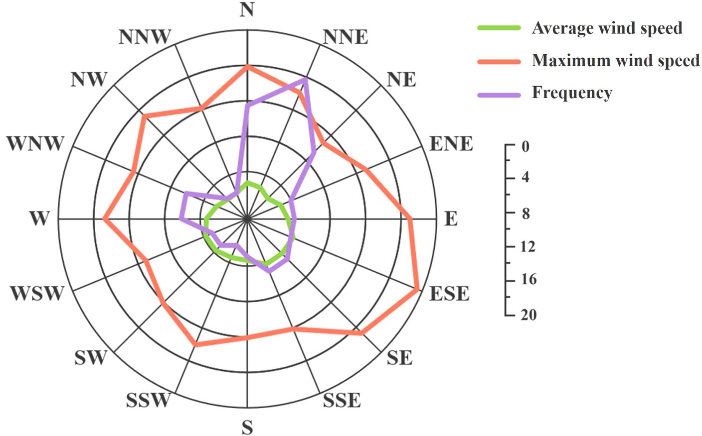
Measured data from July 2003 to May 2005 at Lanshan station indicate that the prevailing wind direction is NNE, with a frequency of 16% (Figure 1). The secondary prevailing wind direction is N, with a frequency of 12%. The average wind speed is relatively small, at 4.1 m/s. The monthly average wind speed is peaking in April at 4.7 m/s and reaching its lowest in January at 3.3 m/s. Throughout the year, wind speeds are generally higher in the ESE ∼ SSE direction, averaging 5.2 m/s. The maximum recorded wind speed is 19.4 m/s from the ESE direction.

Figure 1

Figure 1. Wind radar map of Rizhao Lanshan station.

Analysis of measured wave data at Lanshan Station reveals that the waves in the area are primarily wind waves, with significant seasonal variations in wind wave frequency. In spring, wind wave frequencies are relatively uniform across all directions, with higher frequencies in the NNE ∼ NE and SW, and the highest frequency of 8% in the NE. SE ∼ SSE wind waves are also prevalent, each with a frequencies of 5%, while NNW and ENE have the lowest frequencies, not exceeding 1%.

In summer, NE wind waves have a higher frequency of 10%, followed by E and ESE at 8% and 6%, respectively. Wind waves from the WSW ∼ WNW are less than 1%, with no wind waves from the NW ∼ NNW.

In autumn, wind waves from the NNE and N are the most frequent, with frequencies of 10% and 9%, respectively. SSE and SE follow with frequencies of 4%, and other directions do not exceed 3%.

In winter, the pattern is similar to autumn, with wind waves from the NNE and N being prominent at 13% and 10%, respectively, followed by WSW and W at 4% and 5%, respectively. Frequencies from other directions do not exceed 2%.

3 Data and methods

3.1 Processing of shorelines

3.1.1 Remote sensing image

Remote sensing images are characterized by wide coverage, abundant information content, and short update cycles (Feyisa et al., 2014; Belgiu and Drăguţ, 2016). As an efficient and rapid way of information acquisition, remote sensing demonstrates significant advantages in shoreline extraction. With continuous advancements in the remote sensing technology, improvements in the spatial, temporal, and spectral resolutions have greatly enhanced the precision and real-time monitoring capabilities of water resource assessments (Liu et al., 2012; Kankara et al., 2015; Masria et al., 2015).

The remote sensing images used in this study are sourced from the United States’ Landsat series of satellites, part of a long-term Earth observation program managed by the National Aeronautics and Space Administration (NASA). The primary mission of the Landsat series is to collect image data of the Earth’s surface. Since the launch of the first satellite in 1972, the Landsat series has provided a vast repository of Earth surface images, facilitating the acquisition of information on land use, vegetation growth, water body distribution changes, and other related phenomena. This study uses Landsat-5 TM images from 1985 to 2011 and Landsat-8 OLI images from 2013 to 2020. The spatial resolution of the remote sensing images used in this paper is 30 meters, and the temporal resolution is 16 days.

In recent years, cloud-based high-performance data computing platforms have shown a rapid development, providing convenience and technical support for remote sensing data processing and analysis. Among these platforms, Google Earth Engine (GEE) is widely used for processing Earth observation data (Tamiminia et al., 2020). Built on Google’s extensive global server clusters, GEE offers powerful capabilities in data storage, processing, analysis, and result visualization. The platform’s data directory includes a rich array of public databases, such as remote sensing images, terrain, land, meteorology and population data (Gorelick et al., 2017; Genzano et al., 2020). Which have been preprocessed to enhance data accessibility.

This study utilizes the GEE platform to initially extract the required remote sensing images from the Landsat dataset. A cloud mask is applied to remove clouds, and median composites are created to obtain cloud-free images. The Otsu thresholding method, a statistical based image segmentation technique, is used to extract water bodies from the remote sensing images. This method effectively divides the image into background and target parts based on grayscale characteristics, achieving automatic thresholding and segmentation (Ostu, 1979). We combine the Automated Water Extraction Index (AWEI) proposed by Feyisa et al. (2014) with the Otsu threshold method for water extraction. Finally, the binary water-land images are vectorized to obtain polygonal contours of the shoreline.

$\begin{array}{ll}AWE{I}_{\text{nsh}}=4(\rho ban{d}_2-\rho ban{d}_5)-(0.25\rho ban{d}_4+2.75\rho ban{d}_7)& (2)\end{array}$

where ρ is the DN (Digital Number) value of remote sensing image; band₂, band₄, band₅ and band₇ is the reflectance of green, near-infrared, short-wave infrared and mid-infrared bands of remote sensing images, respectively.

3.1.2 Analysis of shoreline

The Digital Shoreline Analysis System (DSAS) is a software extension based on the Esri Geographic Graphics Information System (ArcGIS) (Himmelstoss et al., 2021). DSAS digitizes, analyzes and visualizes shorelines based on remote sensing images, including calculating the time series change rate of shoreline vector (Valderrama-Landeros and Flores-de Santiago, 2019; Matin and Hasan, 2021). It is widely used to analyze historical shoreline changes, such as erosion and accretion, and the effects of human activities or natural factors. DSAS is significant for shoreline management, planning and coastal community risk assessment (Qiao et al., 2018).

The elements used in DSAS calculation are shown in Figure 2. The shoreline calculation of DSAS can be divided into five steps:

Figure 2

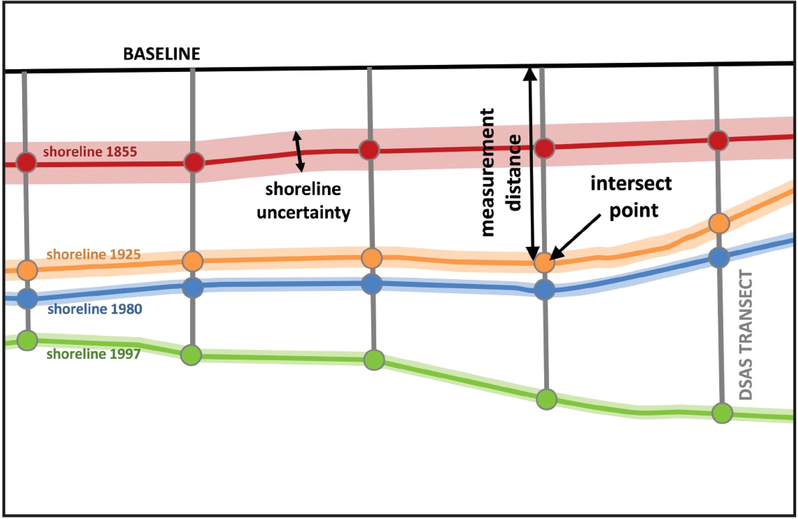
Figure 2. Calculate the distance between baseline and intersect point on different DSAS transects, which can be used to calculate the rate of change of shorelines [Himmelstoss et al. (2021)].

1. Merge multiple shorelines into a shapefile;

2. Create a baseline based on the shoreline;

3. Generate transects;

4. Calculate the shoreline migration distance based on the intersection points of the shorelines and transects;

5. Calculate the shoreline change rate.

In this study, the baseline was set on the landward side, with transects spaced at 30 meters (matching the spatial resolution of Landsat-8). For analyzing shoreline evolution, we utilized three parameters from DSAS: Net Shoreline Movement (NSM), End Point Rate (EPR), and Linear Regression Rate (LRR).

NSM represents the total movement distance of the shoreline over a given time period. When multiple shoreline periods are included, NSM is the distance between the oldest and the youngest shorelines. NSM simply and directly reflects the position changes of two shorelines, but its ability to reflect the trend of shoreline changes is relatively limited.

$\begin{array}{ll}NSM=d_2-d_1& (3)\end{array}$

where $d_1$ is the distance between the oldest shoreline and the baseline, $d_2$ is the distance between the youngest shoreline and the baseline.

EPR is the ratio of NSM to the time interval between the two shorelines, making it easy to calculate. However, when there are a large number of shorelines, some information may be overlooked, such as the rate of shoreline accretion and erosion, and periodic variation trends (Dolan et al., 1991; Crowell et al., 1997).

$\begin{array}{ll}EPR=\frac{d_2-d_1}{t_2-t_1}& (4)\end{array}$

where $t_1$ is the time of the oldest shoreline, $t_2$ is the time of the youngest shoreline.

LRR is calculated through linear regression analysis of shoreline positions at multiple time points. When the dependent variable is the spatial position of the shoreline and the independent variable is the year, the slope of the regression line between the two is representing the LRR. Although this parameter is simple to compute and widely used, it is susceptible to outliers and often lower than other statistical parameters of change rates, such as EPR (Genz et al., 2007). It has significant advantages in calculating and analyzing the rate of change of multiple shorelines over a long period of time.

3.2 Selection of wind datasets

In oceanic and atmospheric scientific research, the ability to accurately reproduce wind fields determines the reliability of numerical simulation results (Kalnay, 2003; Bengtsson et al., 2004). The suitability of reanalysis wind field data often exhibits regional specificity (Hodges et al., 2011; Dukhovskoy et al., 2017). Therefore, selecting appropriate ocean surface wind field data is particularly crucial.

We used measured wind data from Xiaomaidao island (S1) and Lianyungang stations (S2) provided by the North Sea Branch of Ministry of Natural Resources to compare with reanalysis wind data from NCEP CFSV2 and ERA5, in order to analyze the reliability of reanalysis wind fields in the study area of this paper. We calculated the mean absolute error (MAE), root mean square error (RMSE), and correlation coefficient (R) between the measured data and reanalysis datasets at both stations. The calculation formulas are as follows:

$\begin{array}{ll}MAE=\frac{{\sum }^{ }\left|M_i-R_i\right|}{n}& (5)\end{array}$

$\begin{array}{ll}RMSE=\sqrt{\frac{1}{n-1}\left({\sum }^{ }{(M_i-R_i)}^2\right)}& (6)\end{array}$

$\begin{array}{ll}R=\frac{{\displaystyle \sum (M_i-\overline{M})(R_i-\overline{R})}}{\sqrt{{{\displaystyle \sum {(M_i-\overline{M})}^2{\displaystyle \sum {(R_i-\overline{R})}^2}}}^{}}}& (7)\end{array}$

where M is the measured data, R represents reanalysis data, N is the number of samples.

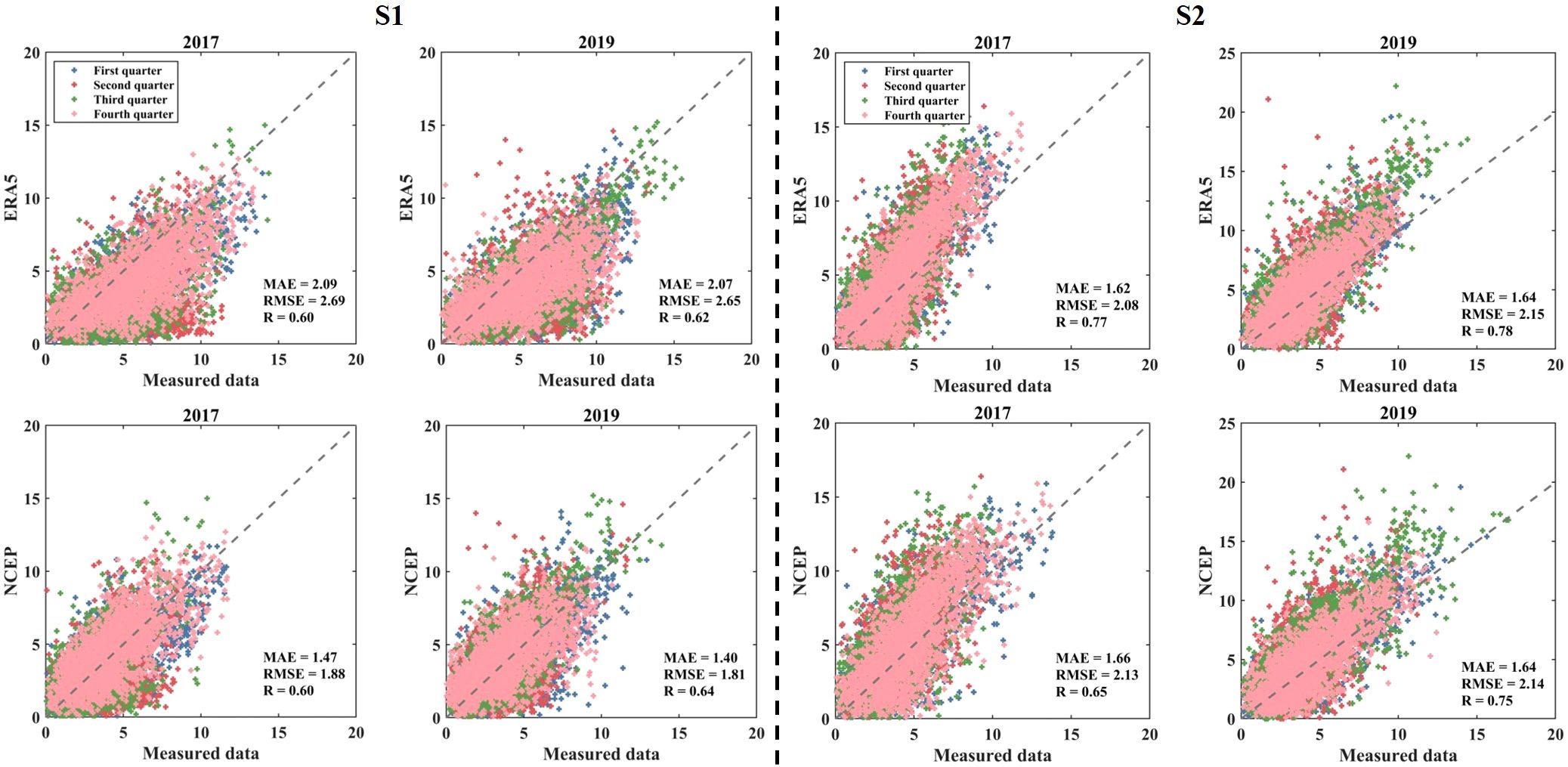
Figure 3 shows the scatter plots of the measured wind speed and reanalysis wind speed at two stations, where blue points represent the first quarter, red points the second quarter, green points the third quarter, and pink points the fourth quarter. Correlation analysis was conducted for the data from 2017 and 2019 at both stations. In 2017, there was no significant impact of typhoon passage in the study area, while Typhoon Lekima passed in August 2019.

Figure 3

Figure 3. Comparison of measured wind speed and reanalysis data from S1 and S2 in 2017 and 2019.

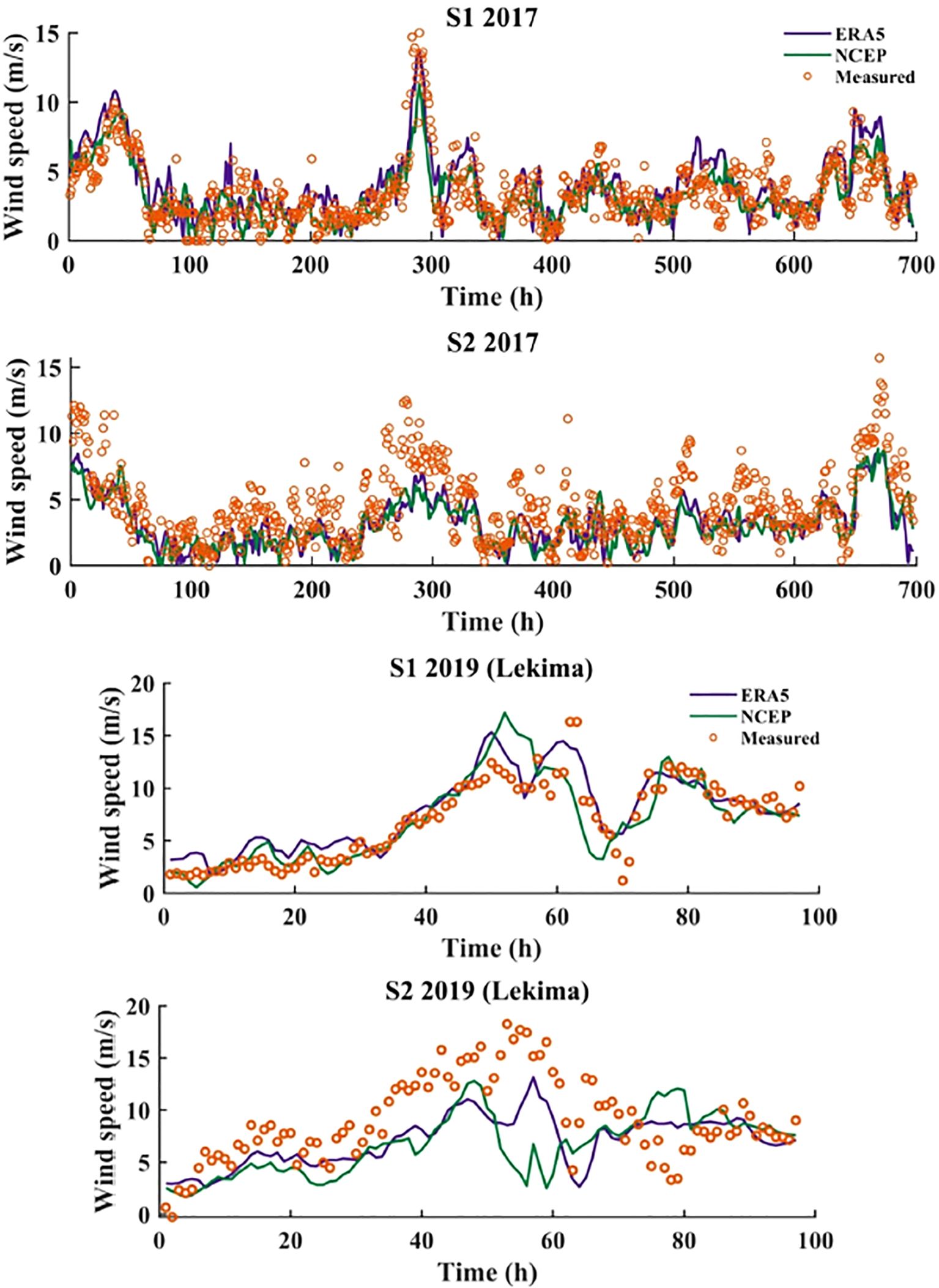
The comparison results of wind speed at S1 indicate that ERA5 underestimates the wind speed, with relatively high MAE and RMSE compared to measured data. Although NCEP performs better at S1, the difference is not substantial. Figure 3 demonstrates that for S2, ERA5 exhibits higher correlation with measured wind speed and lower MAE and RMSE. This advantage is particularly evident in 2017, but not in the typhoon year (2019). Compared to NCEP, ERA5 has lower dispersion and better fitting with measured data (Figure 3). At S2, when wind speeds exceed 7 m/s, both reanalysis wind fields tend to overestimate wind speeds, more pronounced during typhoon periods (third quarter of 2019). To further explore the effect of reanalyzing the wind field on reproducing higher wind speeds, we plotted line scatter plots during periods of high wind speeds (typhoon periods and August in normal years) (Figure 4).

Figure 4

Figure 4. Comparison of wind speeds during strong wind periods at S1 and S2 in 2017 and 2019.

The comparison results of wind speeds at S1 show that both ERA5 and NCEP can accurately reproduce the trend of typhoons. However, ERA5 performs better in reproducing extreme wind speeds, while NCEP tends to underestimate them. Comparison results of wind speeds in August without typhoons (2017) show that both reanalysis wind fields exhibit consistent trends with measured wind fields, and ERA5 still outperforms NCEP in reproducing high winds. Due to the proximity of S2 to the shore, there is a certain deviation between the wind fields of ERA5 and NCEP and the measured wind fields.

After preliminary comparison and analysis, both ERA5 and NCEP show good correlation with measured wind speeds in the study area, and can reproduce wind field trends during typhoon periods and normal years of strong wind periods. However, NCEP tends to underestimate extreme wind speeds, while ERA5 exhibits higher consistency with measured data. Therefore, in this study, we adopt ERA5 reanalysis wind field data.

3.3 Numerical model

Delft3D is a series of hydrodynamic and water environment numerical simulation software developed by Deltares company for estuary, coast and river. It can simulate the processes of water flow, wave, sediment transport, seabed evolution and water quality ecological evolution, as well as the interaction between various processes. Delft3D-flow solves the Navier Stokes equations for an incompressible fluid, according to the Boussinesq assumptions, the ADI (Alternating Direction Implicit) method is used to solve the nonlinear shallow water equation (Deltares, 2014). It can provide real-time hydrodynamic parameters for other models such as wave and sediment. The control equations are as follows:

$\begin{array}{ll}\frac{\partial \eta }{\partial t}+\frac{\partial (hu)}{\partial x}+\frac{\partial (hv)}{\partial y}=0& (8)\end{array}$

$\begin{array}{ll}\begin{array}{c}\frac{\partial v}{\partial t}+u\frac{\partial u}{\partial x}+v\frac{\partial v}{\partial y}+g\frac{\partial \eta }{\partial x}+c_f\frac{v\sqrt{u^2+v^2}}{h}-{\nu }_H(\frac{{\partial }^{2}v}{\partial x^2}+\frac{{\partial }^{2}v}{\partial y^2})\hfill \\ =-fu+M_y\hfill \end{array}& (9)\end{array}$

$\begin{array}{ll}\begin{array}{c}\frac{\partial u}{\partial t}+u\frac{\partial u}{\partial x}+v\frac{\partial v}{\partial y}+g\frac{\partial \eta }{\partial x}+c_f\frac{u\sqrt{u^2+v^2}}{h}-{\nu }_H(\frac{{\partial }^{2}u}{\partial x^2}+\frac{{\partial }^{2}u}{\partial y^2})\hfill \\ =fv+M_x\hfill \end{array}& (10)\end{array}$

where $c_f$ is calculated using the manning coefficient:

$\begin{array}{ll}{c}_f=g\frac{n^2}{\sqrt[3]{h}}& (11)\end{array}$

where, η is water level (m), h is water depth (m), u and v are the vertical average velocity in x and y directions, respectively. $c_f$ is dimensionless friction coefficient, n is manning coefficient (s/m^1/3), ${\nu }_H$ is horizontal eddy viscosity coefficient (m²/s), f is coriolis force coefficient (1/s), $M_x$ and $M_y$ are external momentum source sink term in x and y directions (m/s²), respectively.

SWAN is a wave prediction model developed by Technische Universiteit Delft in the Netherlands. The stochastic wave field is described by a two-dimensional wave action density $N(\sigma ,\theta )$ equilibrium equation based on the Euler approximation. The governing equation is expressed as:

$\begin{array}{ll}\frac{\partial }{\partial t}N+\frac{\partial }{\partial x}{c}_{x}N+\frac{\partial }{\partial y}{c}_{y}N+\frac{\partial }{\partial \sigma }{c}_{\sigma }N+\frac{\partial }{\partial \theta }{c}_{\theta }N=\frac{S}{\sigma }& (12)\end{array}$

where N is action density, which is a function of angular frequency (σ) and direction (θ):

$\begin{array}{ll}N(\sigma ,\theta )=\frac{E(\sigma ,\theta )}{\sigma }& (13)\end{array}$

where $c_i$ represent the transport velocity in x, y, σ and θ. E is energy density. The S on the right-hand side of the equation represents the energy source and sink term:

$\begin{array}{ll}S=S_{in}+S_{nl}+S_{ds}+S_{bot}+S_{surf}& (14)\end{array}$

where $S_{in}$ presents the source generated by wind, $S_{nl}$ represents non-linear wave-wave interaction, $S_{ds}$ represents the dissipation by white capping, $S_{bot}$ represents the dissipation by bottom friction, $S_{surf}$ represents the breaking caused by shallow water depth.

4 Analysis of shoreline change

The change of shoreline reflects the trends in estuarine coastal areas under natural conditions and human activities (Li et al., 2014; Castelle et al., 2018). Studying the shoreline change process is crucial for the conservation of coastal ecosystems and sustainable utilization of marine resources (Qiao et al., 2018; Vitousek et al., 2023). This section extracts shoreline data from Landsat series remote sensing images spanning from 1985 to 2020, analyzing 35-year variations of shoreline changes. Additionally, it examines monthly shoreline changes during a dry year (2015), a wet year (2020), and a typhoon year (2019) to explore the seasonal variations of different typical years.

4.1 Shoreline change trend

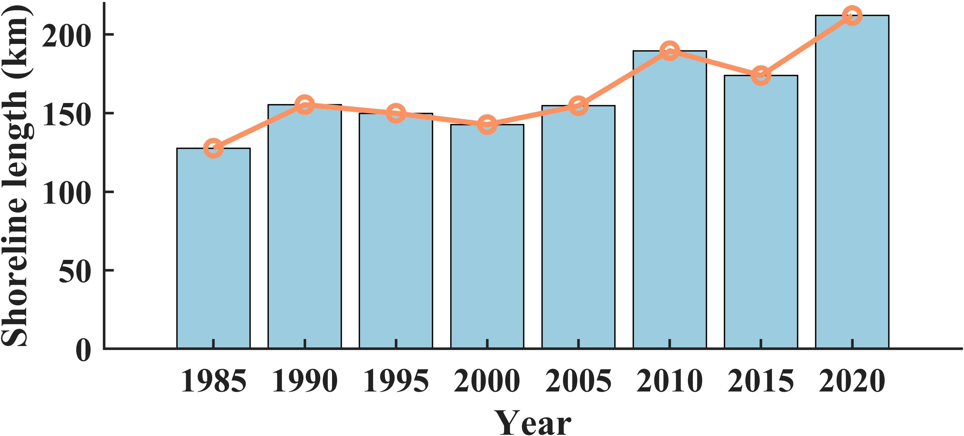
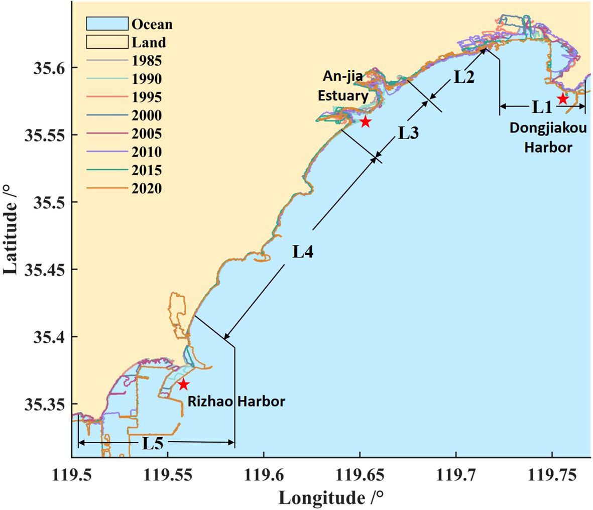
Using the GEE platform, we extracted and processed shoreline data from Landsat remote sensing images, obtaining annual average shorelines for the study area from 1985 to 2020. The shoreline extends from Rizhao harbor in the south to Dongjiakou harbor in the north. The total length of the shoreline increased from 127.7 km in 1985 to 155.4 km in 1990, then decreased to 149.9 km in 1995 and 142.7 km in 2000. In 2005 and 2010, the coastline increased to 154.7 km and 189.7 km, respectively, and then decreased again. In 2015, the total length was 173.9 km, finally increased to 212.1 km in 2020. Although the length fluctuates, it exhibits an overall increasing trend (Figure 5).

Figure 5

Figure 5. Change in total length of shorelines.

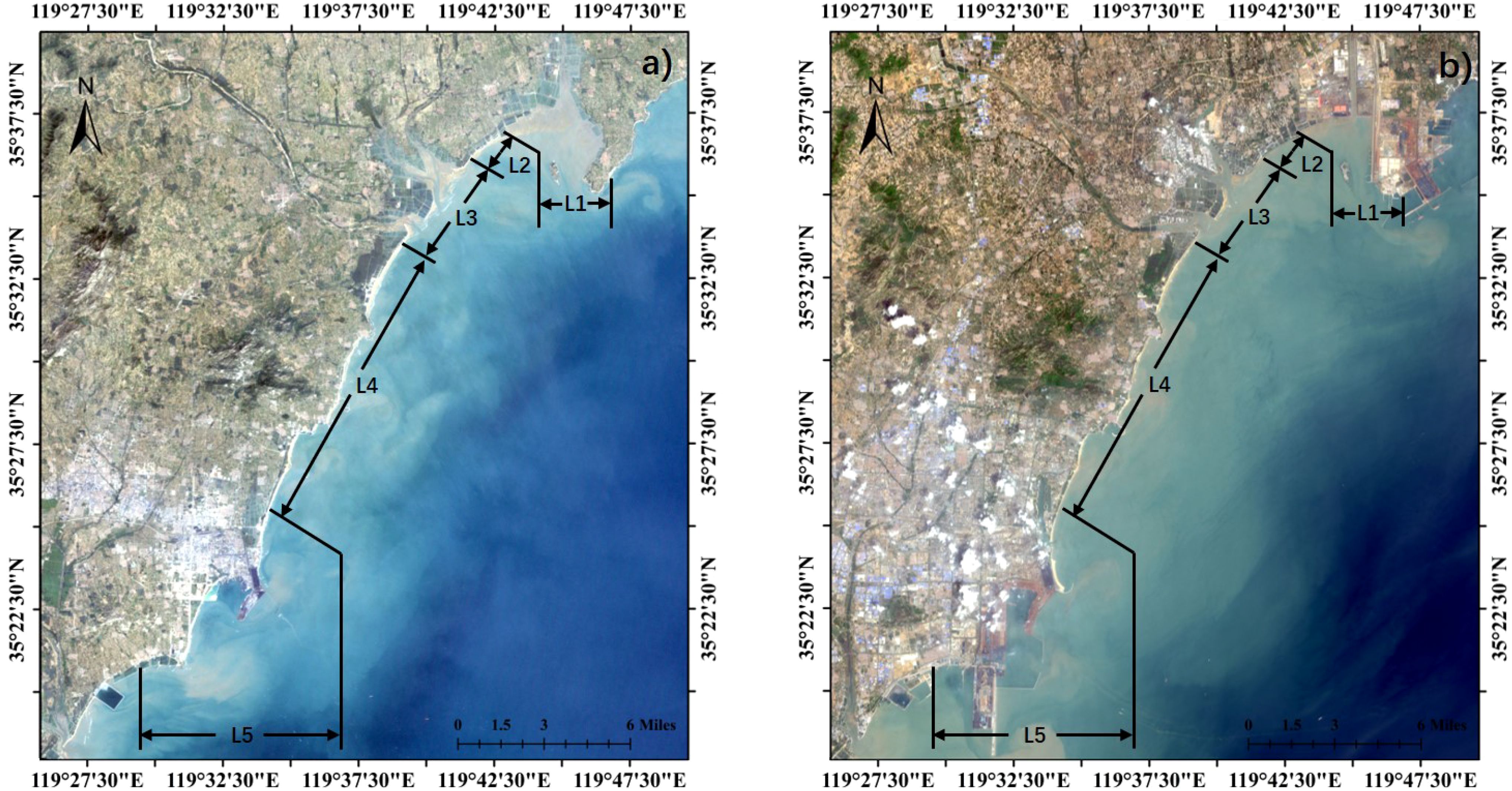
To analyze the trend of shoreline changes over the past 35 years, we plotted and compared the shoreline changes every five years. To further clarify regional variation of the shoreline and explore the reasons for shoreline changes, we divide the shoreline into five segments (L1 ∼ L5) based on geological characteristics and the magnitude of shoreline changes (Figure 6). The L1 and L5 shorelines have been greatly affected by human activities, while the L2 ∼ L4 shorelines are relatively natural shorelines. Due to the winding changes in shorelines at the estuaries, we have divided them into a separate segment (L3). L1 includes the Dongjiakou harbor area; L2 comprises the fishery aquaculture area between Dongjiakou harbor and the estuaries; L3 encompasses two estuaries within the study area; L4 consists of relatively straight sandy beaches; and L5 includes the Rizhao harbor area. From Figure 7, it is observed that shoreline changes in L2 and L4 are relatively small, with a high degree of overlap over the past 35 years. The overall shape of the estuaries in L3 has not changed significantly, only showing moderate erosion and deposition. Due to the construction and improvement of two harbors, the shorelines in L1 and L5 have experienced significant changes over the past 35 years.

Figure 6

Figure 6. Remote sensing image of study area [(A) September 2000, (B) May 2020].

Figure 7

Figure 7. 35 year shoreline distribution of the study area (with an interval of five years).

The changes in the L1 and L5 shorelines are attributed to harbor construction. The construction of Dongjiakou harbor, which commenced in May 2009 and was completed in March 2013, led to significant changes in the L1 shoreline. L5 shoreline is located in Rizhao harbor area, which began construction in 1982 and was completed and operational in 1986. Since then, Rizhao harbor has undergone continuous construction and repair. In addition to port construction, a series of coastal protection projects have also been carried out, resulting in complex changes in the L5 shoreline. After the construction of harbors, artificial shorelines replace natural ones, and the shoreline length tends to stabilize with no significant erosion or deposition.

Field surveys revealed that the L2 shoreline is a natural fishery aquaculture area with minimal tourism development, preserving coastal beaches and exhibiting a natural shoreline state. The L2 shoreline is located within Qizi Bay and is protected by a cape. This segment experiences significant seasonal erosion and deposition, but minimal annual fluctuations. The L3 area consists of two estuaries formed by the Liangcheng River, Baima River, and Jili River. The runoff of these rivers shows significant seasonal changes, with peak runoff in summer (July-August) and smaller runoff in other seasons. Compared to other segmented shorelines, the L2 and L3 shorelines have fewer artificial structures and less human activity interference, reflecting natural shoreline changes.

The L4 shoreline is relatively straight and mostly composed of sandy coasts. Since 1985, except for the construction of a tourist fishing port, there have been no significant changes in the shoreline. This stability is due to extensive tourism development in the area, with protective structures built behind the beach, further weakening the impact of waves on the shoreline. The total length of the L4 shoreline exhibits minimal fluctuations, and the shoreline position remains relatively stable. The magnitude of erosion and deposition along the L4 shoreline has not changed much. From 1985 to 2020, the average erosion and deposition values of the shoreline every five years were 2.01 m, -29.56 m, 15.25 m, -6.85 m, 12.14 m, -37.32 m, and 50.00 m (positive values represent seaward deposition and negative values represent landward erosion). The maximum average change in shoreline occurred during the period of 2015-2020, with a seaward deposition of 50 m, attributed to the construction of the tourist fishing port project, leading to a shoreline advance of approximately 623.31 m. Therefore, apart from human activities, the overall changes in the L4 shoreline are not significant and relatively stable.

4.2 Shoreline change rate

To quantitatively analyze the shoreline changes in the study area, we imported the shorelines from 1985 to 2020 into ArcGIS and used DSAS to calculate the shoreline change rate. DSAS requires smooth shorelines for accurate calculations; sinuous shorelines can result in larger errors and outliers. Our study focused on erosion and deposition the two estuaries in Qizi Bay, so we primarily analyzed changes in L1, L2, L3, and the northern half of L4 (labeled as L4-1). Among these segments, L1 and L3 exhibit complex morphologies, while L2 and L4-1 are relatively smoother. Consequently, DSAS was applied only to L2 and L4-1 for shoreline change calculations, while the analysis of L1 and L3 focused on describing morphological changes.

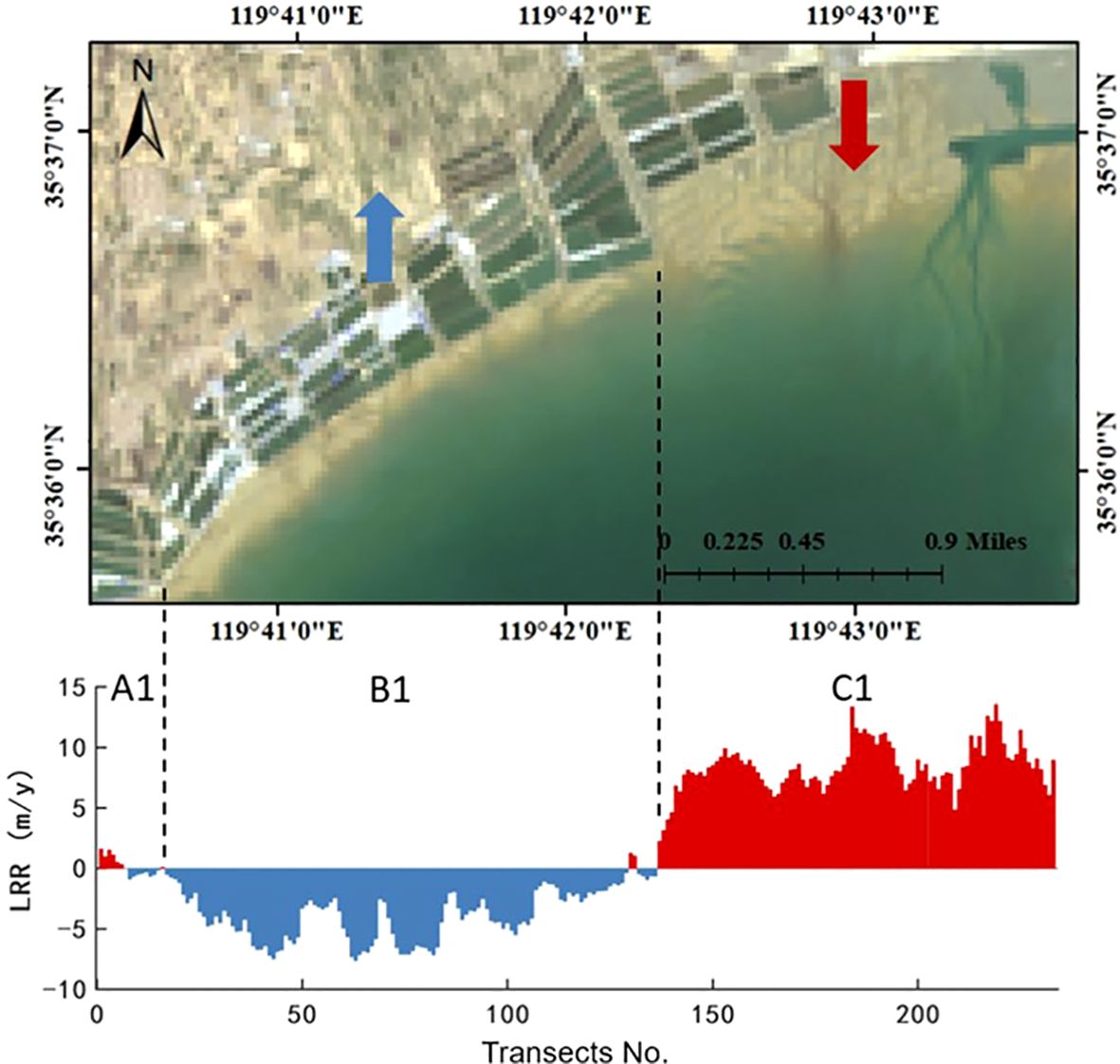
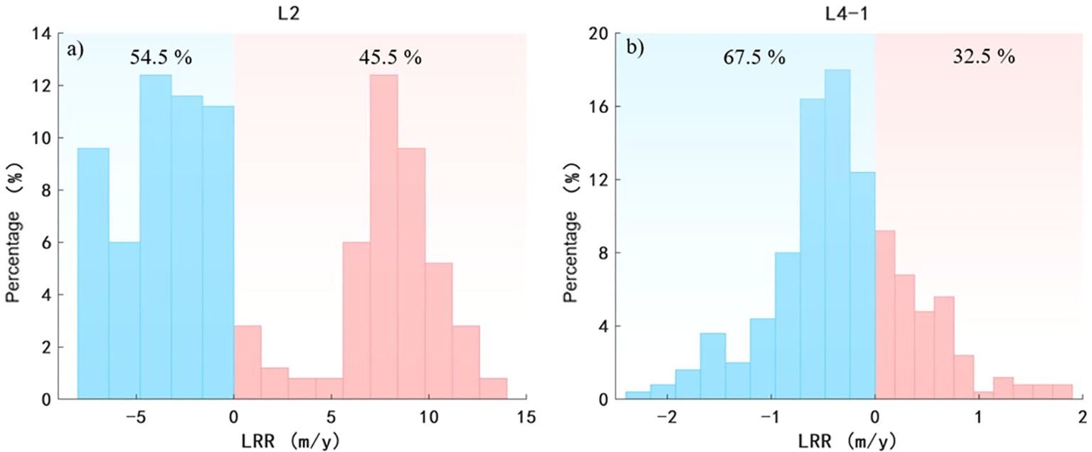
Figure 8 illustrates the alongshore distribution of the LRR for the L2 shoreline. The L2 shoreline exhibits pronounced erosion and deposition segments. Negative LRR values indicate landward erosion, while positive values indicate seaward deposition. The maximum erosion of L2 shoreline occurs within B1, with an LRR value of -7.62 m/year, while the maximum deposition occurs within C1, with an LRR value of 13.54 m/year. The average LRR for the entire L2 shoreline is 1.54 m/year. Among them, 45.5% of the shoreline experiences seaward deposition, while 54.5% experiences landward erosion, with shoreline erosion and deposition proportions being relatively balanced (Figure 9A).

Figure 8

Figure 8. LRR distribution map of each transect of L2 shoreline.

Figure 9

Figure 9. LRR histograms of L2 (A) and L4-1 (B) shorelines.

The southern section of the L2 shoreline (A1) is adjacent to the estuaries, and exhibits alternating erosion and deposition due to the influence of runoff. The B1 shoreline, farther away from the estuaries, shows a stable landward erosion. B1 is exposed to wave action without the protection of the eastern cape, making it susceptible to the impact of wind and waves. The northern section of the L2 shoreline (C1) shows significant deposition, attributed to the sheltering effect of the cape and Muguan island, facilitating sediment settling within the bay. Additionally, the northern part of L2 shoreline is within the construction scope of Dongjiakou harbor, resulting in significant seaward deposition due to harbor construction activities.

As shown in Figure 10, the LRR of the L4-1 shoreline is significantly lower than that of the L2 shoreline, indicating smaller annual variation relative stability. Within the L4-1 shoreline, the maximum erosion occurs within C2, with an LRR of -2.27 m/year, while the maximum deposition occurs within B2, with an LRR of 1.87 m/year. The average LRR for the entire L4-1 shoreline is -0.27 m/year. Among them, 32.5% of the shoreline experiences seaward deposition, while 67.5% experiences landward erosion, with erosion being the dominant process, accompanied by localized deposition (Figure 9B). Moving from south to north, the L4-1 shoreline initially undergoes minor erosion (A2), typical of normal shoreline changes. The northern protrusion (B2) is Renjiatai Reef Park in Rizhao. The cape is located at the wave convergence area, which shares the impact of waves with the beaches on both sides. Therefore, the two sides of the cape show the seaward deposition. The middle-upper section of the L4-1 shoreline (C2) is mainly characterized by erosion. This part of shoreline comprises sandy beaches without significant shelter, where shoreline changes are driven by various hydrodynamic factors. The last section of the shoreline (D2) is close to the estuaries and is greatly affected by theme, exhibiting alternating erosion and deposition patterns.

Figure 10

Figure 10. LRR distribution map of each transect of L4-1 shoreline.

We calculated and plotted the End Point Rate (EPR) of the L2 and L4-1 shorelines every five years over a 35 year period (Figure 11) to further explore shoreline changes from 1985 to 2020. From Figure 11, it is evident that the EPR for the L2 shoreline is significantly higher than for L4-1, indicating more pronounced changes for L2. Transects 1-126 exhibit alternating erosion and deposition over the 35-year period. This area is primarily used for natural fishery cultivation, and the shoreline changes are predominantly influenced by hydrodynamic factors. Transects 126-233 experience larger EPR values, mainly due to their location within the enclosed Qizi Bay, where complex hydrodynamic conditions disturb shoreline changes. Between 2010 and 2015 (gray line), this section of L2 shoreline was affected by the construction of Dongjiakou harbor, resulting in significant seaward deposition (Figures 12A, B). The L4-1 shoreline, being smooth and mainly composed of sandy beaches, shows EPR fluctuates between -40 ∼ 40 m/y, with regular changes and no extreme changes.

Figure 11

Figure 11. The EPR distribution of L2 (A) and L4-1 (C) shorelines (interval of 5 years). The shoreline near the estuaries is marked using a red box and enlarged (B, D).

Figure 12

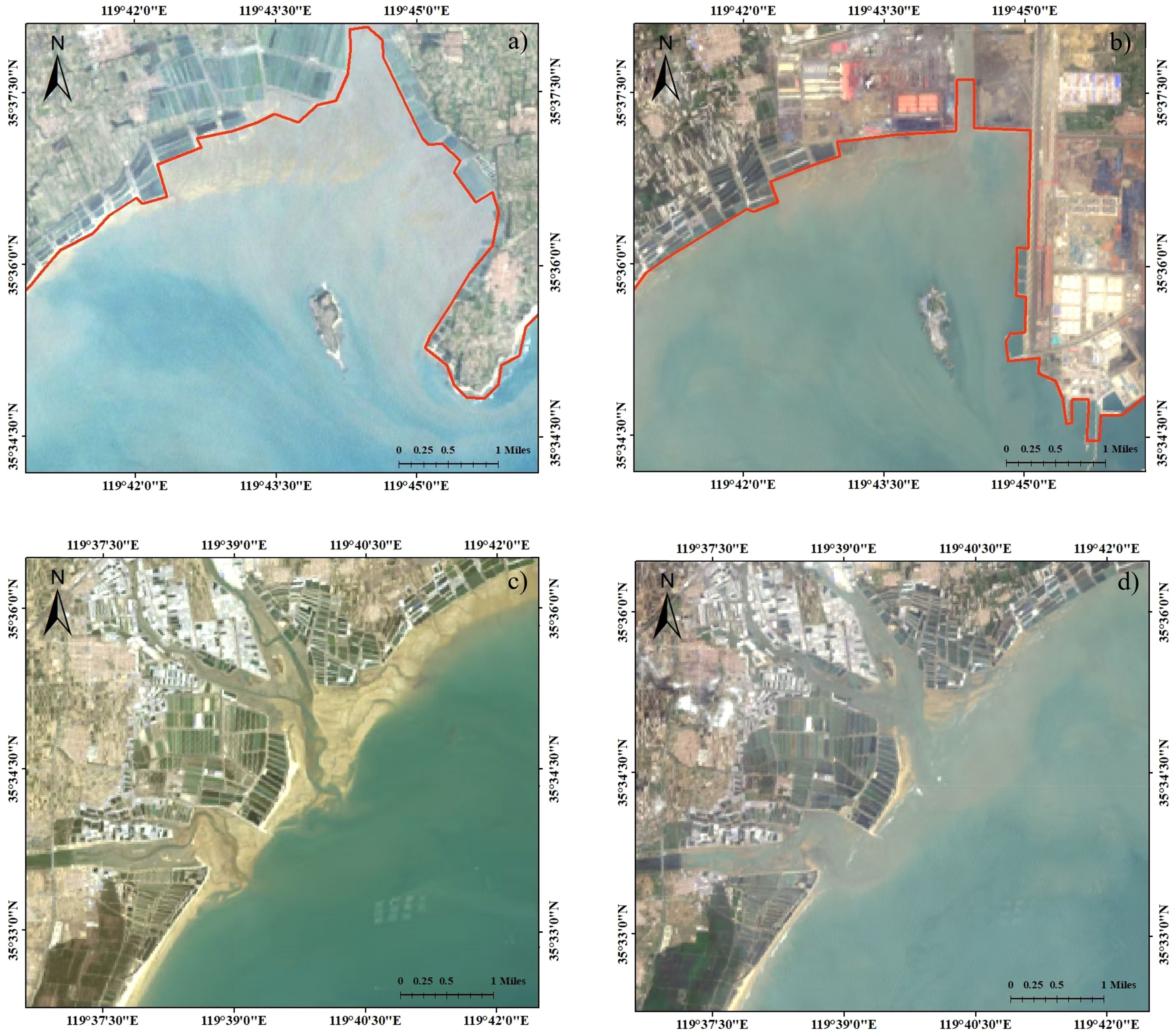
Figure 12. (A, B) is the remote sensing image of Dongjiakou harbor [(A) September 2000, (B) May 2020]. (C, D) are remote sensing images of the estuaries area [(C) March 2020, (D) May 2020].

To analyze the shoreline changes near the estuaries, we enlarged the EPR distribution for the L2 and L4-1 segments near the estuaries (Figures 11B, D). The EPR of the two shorelines is similar, except for significant deposition in L2 between 2015 and 2020. In all other periods, the EPR is between -40 ∼ 40 m/y. Figure 11B is close to the north estuary, while Figure 11D is close to the south estuary. The latter fluctuates more violently, possibly due to the steeper slope before the south estuary. Comparison of the estuarine areas in remote sensing images (Figures 12C, D) revealed clear seasonal variations in shoreline changes. As our study employs annual average shorelines, the alternation of erosion and deposition near the estuaries is a normal phenomenon.

Figures 12A, B, illustrate that harbor construction resulted in artificial shorelines replacing natural ones, altering shoreline characteristics. The port construction led to significant seaward accretion, with a maximum distance of approximately 1248 m. Additionally, we compared shoreline changes over 35 years in the estuaries region and found no significant changes in estuarine morphology or estuarine diversion. Figures 12C, D show remote sensing images of March and May 2020, respectively, illustrating that shoreline changes at the estuaries vary greatly during different seasons. Hence, we will explore the seasonal changes of the shoreline in the study area within a year in the next section.

4.3 Seasonal variation of shoreline

To further explore the variation pattern of the shoreline, this section discusses the seasonal changes of the shoreline in typical years. Considering runoff as one of the influencing factors on shoreline migration, we selected the dry year (2015) and the flood year (2020) as typical years to analyze and compare the seasonal changes of the shoreline. In 2015, a severe drought year in Shandong Province, the annual river discharge into the sea was only 4.8% of that in 2020, according to statistics from the Rizhao Hydrological Bureau and the Qingdao Hydrological Bureau. Moreover, there were no major coastal engineering projects conducted in either 2015 or 2020, allowing for a comparison of shoreline erosion and deposition.

Shoreline changes represent the specific manifestation of the interaction of dynamic factors in coastal areas. Therefore, it is necessary to analyze the changes in dynamic factors in the study area to explain the changes in the shoreline. However, the study area lacks long-term wave and hydrological observation stations, and commonly used international reanalysis databases generally have low spatial resolutions (e.g., ERA-5 wind data with a spatial resolution of 0.25° and wave data of 0.5°). With appropriate parameter settings, numerical models can effectively reproduce the dynamics of relevant areas. The Delft3D model has high credibility and wide application in coupled wave-current numerical simulations (Hibma et al., 2004; Lesser et al., 2004; Marciano et al., 2005), so we use the Delft3D model for numerical simulation of wave-current coupling in the study area.

The simulation area of the model includes the Bohai Sea and parts of the Yellow Sea in China, with regional grid refinement for the study area (Figure 13). The water depth data is taken from the 2018 digital nautical chart. The hydrodynamic boundary is set on the south side, with tidal and wave boundary conditions applied. The tidal boundary conditions were driven by the harmonic analysis constants of eight common tidal constituents (K1, K2, M2, N2, O1, P1, Q1, S2) from NAO.99b (Matsumoto et al., 2000), and the wave boundary conditions were based on ERA-5 reanalysis wave data. Additionally, ERA-5 reanalysis wind field data were added to the model as driving conditions.

Figure 13

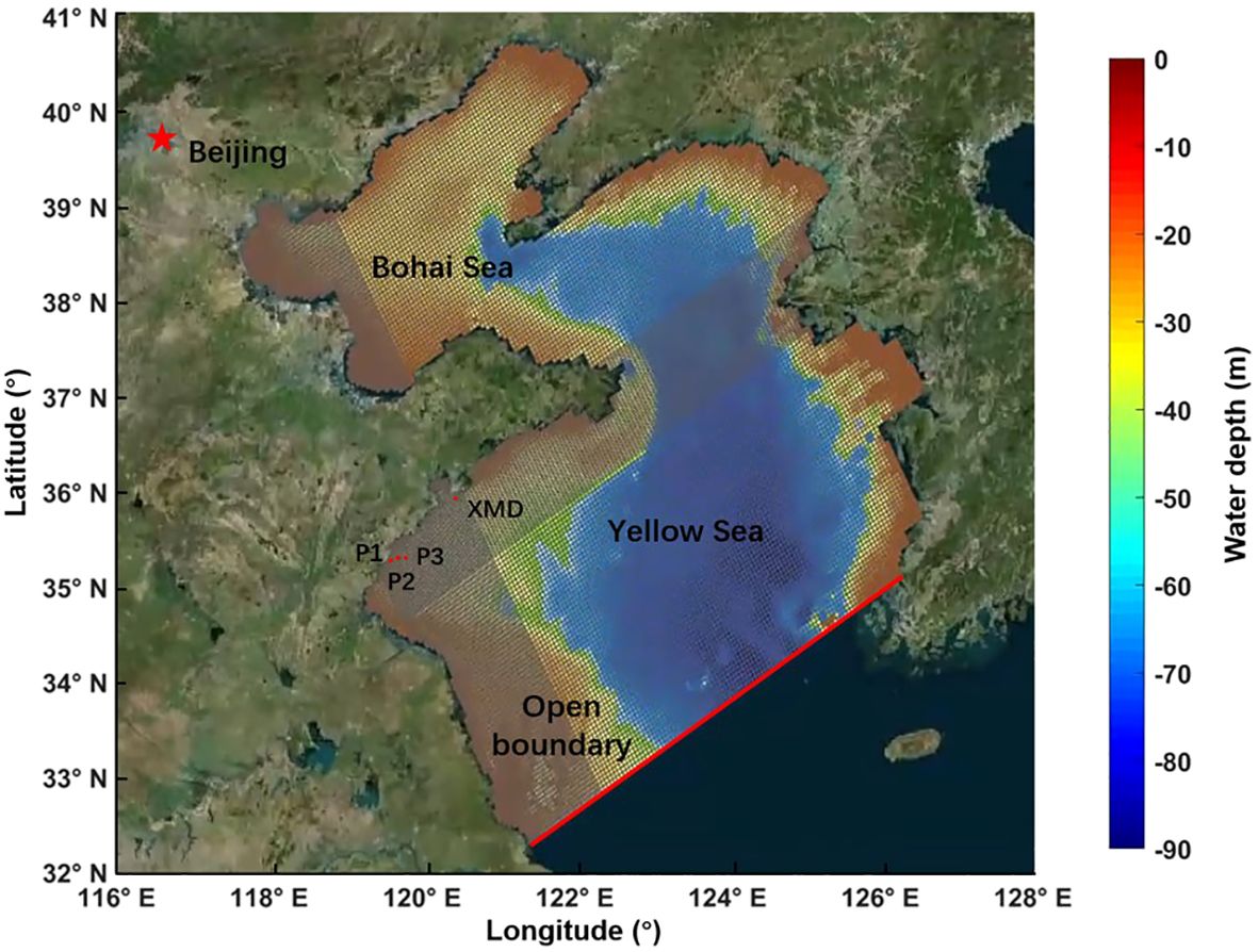
Figure 13. Delft3D computational grid and water depth distribution map. P1-P3 are the measured points of the current, XMD is the position of the wave observation station, and the open boundary of the model is marked in red line.

To ensure the accuracy of the model in reproducing hydrodynamics in the study area, the model was calibrated using measured data near the study area. Current and water level data were obtained from observations (Point 1 to Point 3 in Figure 13) conducted by the Ocean University of China in August 2015 in the Rizhao Sea area, while wave and wind observation data were from the Xiaomaidao (XMD in Figure 13) island wave observation station. After parameter tuning, the simulated data showed a high degree of agreement with the observed data (Figure 14), indicating the high reliability of the numerical simulation results.

Figure 14

Figure 14. The validation of wind and wave (XMD).The validation of water level and current (P1-P3). The blue solid line is the simulated value, and the red scatter is the measured value.

We compared the correlation between NSM and various dynamic factors in the study area and found that runoff had the highest correlation (Figure 15). This is likely because runoff carries sediment from upstream into the sea. The third and fourth quarters of 2020 were excluded from the correlation analysis due to extreme runoff in Q3, which resulted in significant sediment loss in the channel. Despite higher runoff in Q4, the shoreline still exhibited erosion toward the land. These two points are not representative and were therefore excluded from the correlation analysis.

Figure 15

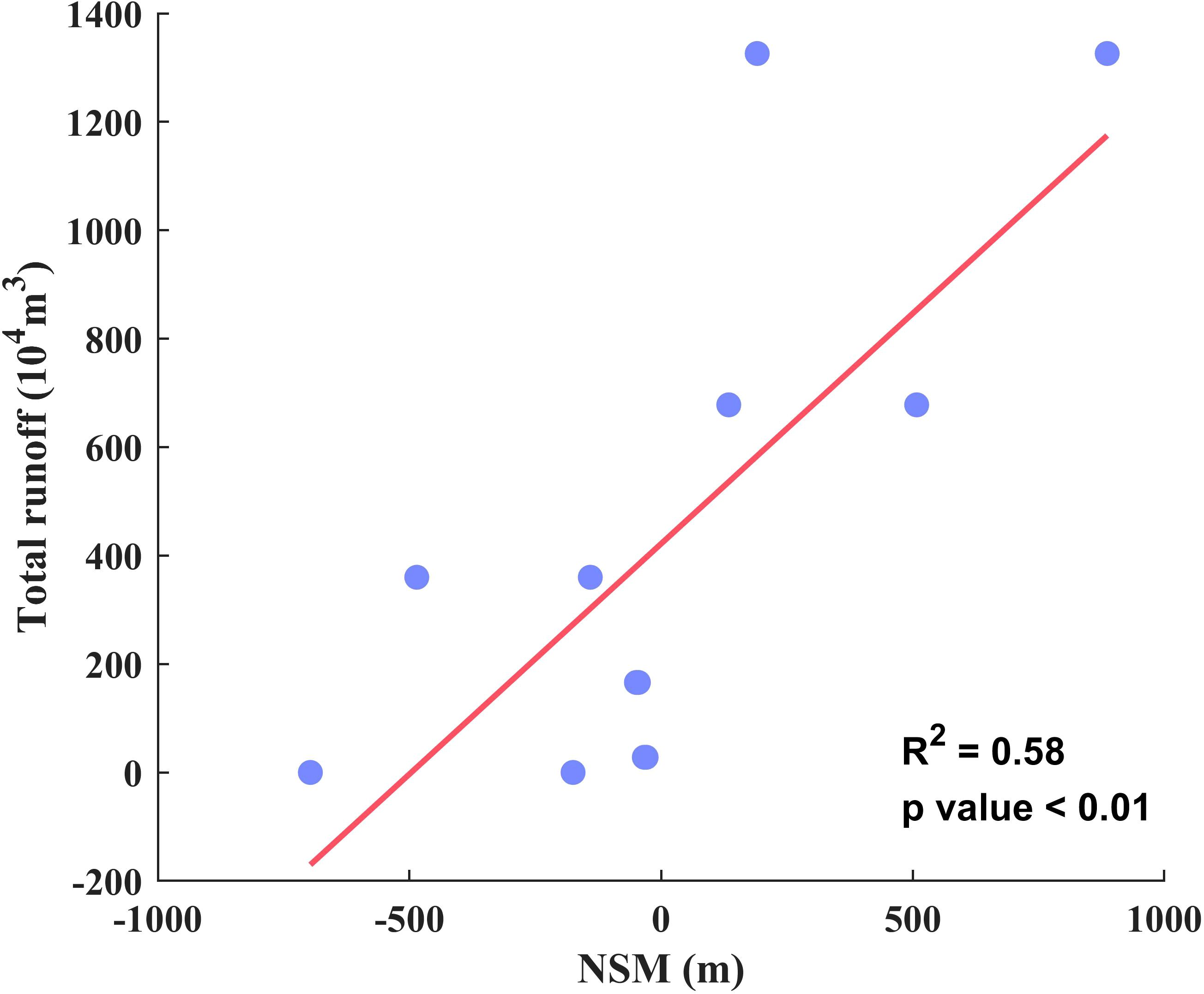
Figure 15. Correlation analysis between runoff and NSM. The horizontal axis represents the average NSM within a quarter, while the vertical axis represents the total runoff within a quarter.

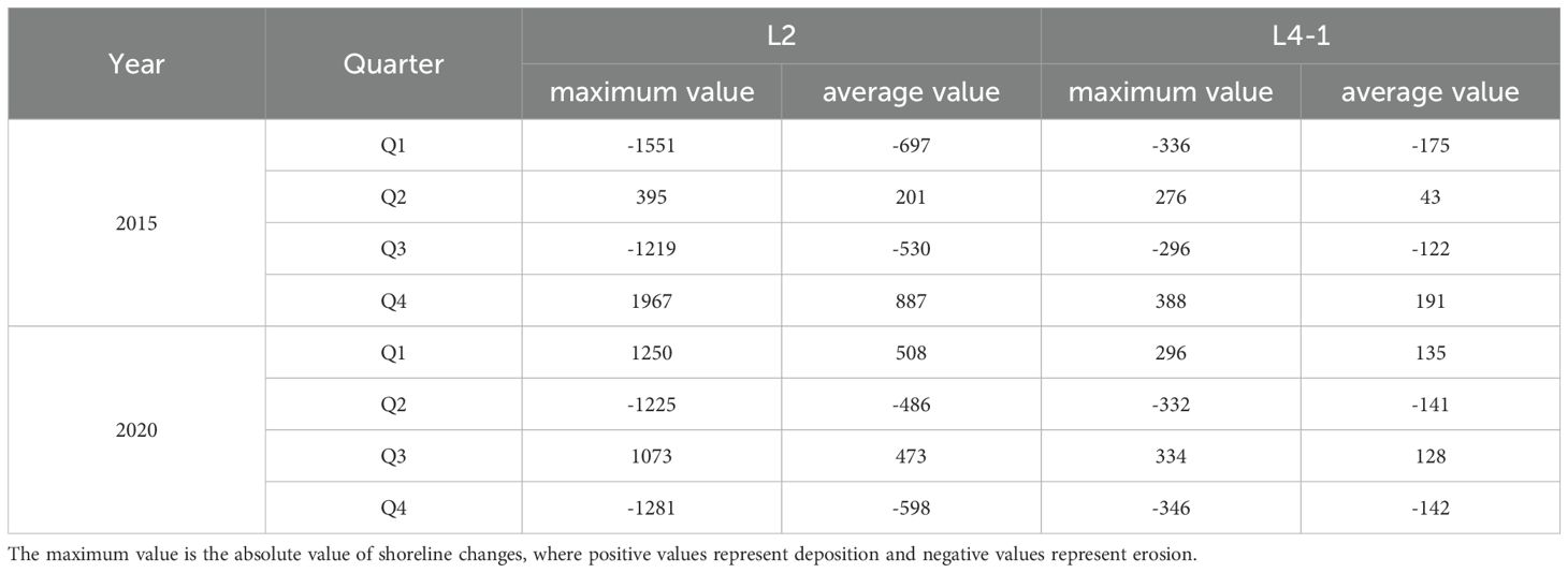
Figure 16 shows the net shoreline movement (NSM) of the L2 and L4-1 shorelines in different quarters of 2015 and 2020. Table 1 lists the maximum and average values of NSM in Figure 16. Positive values represent deposition toward the sea, while negative values indicate erosion toward the land. In the first quarter (Q1) of 2015, estuaries were cut off, resulting in shoreline erosion due to the lack of upstream sediment supply and increased wave and wind intensity from Q1 to Q2. In Q1 of 2020, despite a slight increase in wave and wind intensity compared to 2015, the shoreline still experienced accretion, likely due to sediment supply from upstream rivers. In the second quarter (Q2) of 2015, partial river runoff resumed, alleviating shoreline erosion, although the runoff was small. During Q2 of 2020, runoff decreased compared to Q1, and wind and wave intensities were significantly higher, leading to shoreline erosion toward the land.

Figure 16

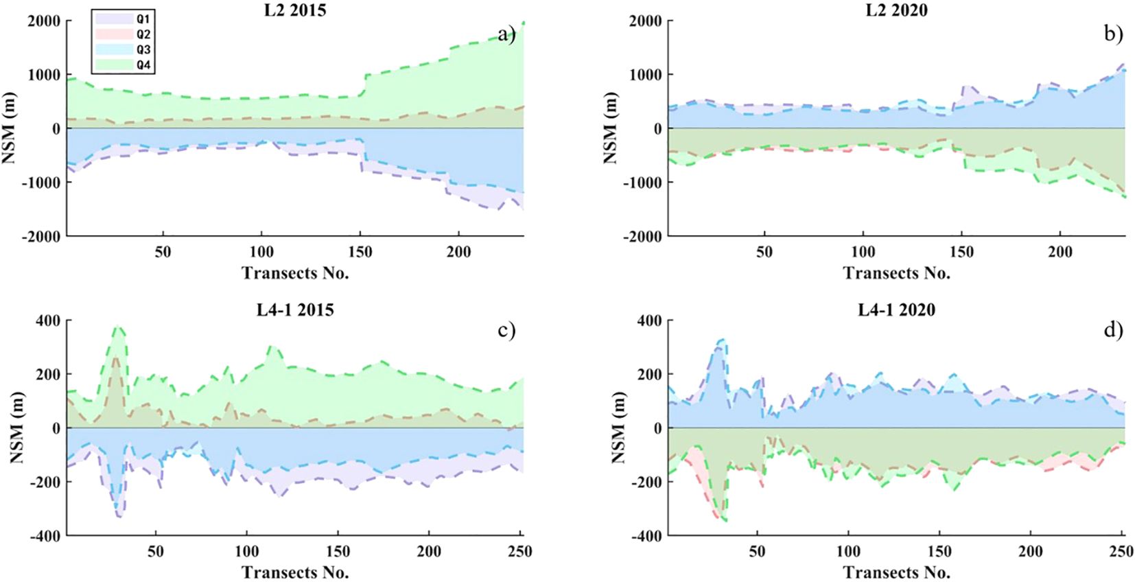
Figure 16. The net shoreline movement (NSM) of different quarters in 2015 and 2020. (A, B) represent L2 shoreline NSM, (C, D) represent L4-1 shoreline NSM.

Table 1

Table 1. NSM of L2 and L4-1 shorelines in 2015 and 2020.

In the third quarter (Q3) of 2015, runoff was slightly higher than in Q2, but large wind speeds and waves in July resulted in significant erosion along the shoreline, especially away from the estuaries. During Q3 of 2020, with a significant increase in runoff, the shoreline experienced significant deposition toward the sea. Although the intensity of dynamic factors in Q3 was greater than in Q1, the deposition amplitude in Q3 was comparable to that in Q1 due to the large sediment supply. In the fourth quarter (Q4) of 2015, runoff increased, reaching its maximum for the year, and the intensity of dynamic factors was the smallest, resulting in shoreline deposition toward the sea. In contrast, in Q4 of 2020, runoff decreased, and the large runoff during Q3 had taken away most of the sediment in the river channel. Therefore, the runoff into the sea could not provide sufficient sediment supply for the coast, resulting in shoreline retreat.

We calculated the net shoreline movement (NSM) before and after the passage of Typhoon Matmo (June-July 2014) and Typhoon Lekima (August-September 2019) (Figure 17). Typhoon Matmo (2014), formed in the Northwest Pacific, made landfall in Taiwan, China, on July 23, and subsequently made a second landfall in Rongcheng City, Shandong Province, on July 25. The maximum wind force near the center when landing was 8. Typhoon Lekima (2019), also formed in the Northwest Pacific, made landfall in Zhejiang Province, China, on August 10, and a second landfall along the coast of Qingdao, Shandong Province, on August 11. The maximum wind force near the center when landing was 9. Typhoon Matmo passed through the study area on July 25, 2014, and there was no significant runoff during the period of shoreline change calculation. Therefore, the shoreline changes in Figures 17A, B were mainly caused by the typhoon. The passage of Matmo led to shoreline retreat toward the land, with approximately 100 m of erosion near the estuaries. The maximum erosion occurred near the shoreline adjacent to Qizi Bay, where the shoreline retreated by about 525 m. Typhoon passages often result in extreme sea conditions, causing coastal sediment loss. Coupled with low runoff and lack of timely sediment replenishment, this leads to shoreline retreat in the study area.

Figure 17

Figure 17. The NSM of L2 and L4-1 shorelines during the period of Typhoon Matmo in 2014 and Typhoon Lekima in 2019. (A, B) is the NSM from June to July 2014: (C, D) is the NSM from August to September 2019.

Figures 17C, D shows that the shoreline deposited after the passage of Typhoon Lekima. The shoreline near the estuaries advanced seaward by approximately 60 m, with the maximum accretion occurring near the side adjacent to Qizi Bay, around 225 m. After consulting the runoff data, it was found that after the Lekima transit, a large-scale rainfall occurred in the study area, and the runoff increased significantly. The runoff transported sediment to both sides of the coasts, making up for the erosion of the shoreline by the typhoon. Despite this, the monthly deposition during the period of Lekima is significantly smaller than the quarterly average deposition (Figures 17C, D), indicating that the typhoon has greatly inhibited the deposition of coastal sediment.

5 Conclusion

Through a comparison of shorelines from 1985 to 2020, we found that significant shoreline changes in the study area were primarily due to human activities such as harbor construction. In contrast, the natural shoreline showed high consistency over the 35 years. Further analysis of the shorelines on both sides of the estuaries revealed that the southern shoreline (L4-1) had a relatively open sea area and a straight shoreline with minimal overall change, predominantly exhibiting shoreline erosion. The northern shoreline (L2), near the cape and Muguan Island, showed greater variation, likely due to the complex dynamic environment in the bay, with an equal proportion of erosion and deposition.

The study area contains seasonal estuaries, so we analyzed the intra-annual shoreline changes during dry and wet years, respectively. The erosion and deposition trends during the same seasons in dry and wet years were not consistent. Therefore, we analyzed the correlation between the Net Shoreline Movement (NSM) and dynamic factors for each year. The results showed a high correlation between NSM and runoff, which is considered to be caused by the upstream sediment carried by the runoff into the sea, with sections near the estuaries being the most sensitive to the changes in runoff. The results showed a high correlation between NSM and runoff, likely due to the river carrying upstream sediments into the sea. Additionally, NSM was influenced by other dynamic factors such as wave intensity. Therefore, we analyzed the NSM during two typhoons that passed through the study area. The results indicated that typhoons caused rapid shoreline erosion in the short term, but sediment-laden runoff mitigated this erosion. Thus, the change of shoreline is not only controlled by a single dynamical factor, but is a manifestation of the interaction of multiple dynamical factors.

In future work, we will incorporate high-resolution temporal and spatial data to capture short-term events and their direct impact on shoreline dynamics. Combining flow-wave-sediment modeling with empirical observations will provide a deeper understanding of the driving mechanisms behind shoreline changes. A comprehensive analysis of shoreline evolution will enhance our ability to protect and sustainably manage coastal areas.

Data availability statement

The raw data supporting the conclusions of this article will be made available by the authors, without undue reservation.

Author contributions

ZZ: Software, Writing – review & editing, Writing – original draft, Methodology. ZW: Writing – review & editing, Supervision, Methodology, Funding acquisition. BL: Writing – review & editing, Visualization, Funding acquisition, Conceptualization. XL: Writing – review & editing, Investigation, Data curation. BY: Writing – review & editing, Software, Formal Analysis. LS: Writing – review & editing, Visualization, Validation.

Funding

The author(s) declare financial support was received for the research, authorship, and/or publication of this article. The author would like to acknowledge the support of the National Natural Science Foundation of China (Grant No.52101338, No.52301345, No.52201341).

Conflict of interest

The authors declare that the research was conducted in the absence of any commercial or financial relationships that could be construed as a potential conflict of interest.

Publisher’s note

All claims expressed in this article are solely those of the authors and do not necessarily represent those of their affiliated organizations, or those of the publisher, the editors and the reviewers. Any product that may be evaluated in this article, or claim that may be made by its manufacturer, is not guaranteed or endorsed by the publisher.

References

Addo K. A., Walkden M., Mills J. T. (2008). Detection, measurement and prediction of shoreline recession in Accra, Ghana. ISPRS J. Photogramm. Remote Sens. 63, 543–558. doi: 10.1016/j.isprsjprs.2008.04.001

Crossref Full Text | Google Scholar

Alesheikh A. A., Ghorbanali A., Nouri N. (2007). Coastline change detection using remote sensing. Int. J. Environ. Sci. Technol. 4, 61–66. doi: 10.1007/BF03325962

Crossref Full Text | Google Scholar

Belgiu M., Drăguţ L. (2016). Random forest in remote sensing: A review of applications and future directions. ISPRS J. photogramm. Remote Sens. 114, 24–31. doi: 10.1016/j.isprsjprs.2016.01.011

Crossref Full Text | Google Scholar

Bengtsson L., Hodges K. I., Hagemann S. (2004). Sensitivity of large-scale atmospheric analyses to humidity observations and its impact on the global water cycle and tropical and extratropical weather systems in era40. Tellus A: Dynam. Meteorol. Oceanogr. 56, 202–217. doi: 10.1111/j.1600-0870.2004.00053.x

Crossref Full Text | Google Scholar

Bertin X., Castelle B., Chaumillon E., Butel R., Quique R. (2008). Longshore transport estimation and inter-annual variability at a high-energy dissipative beach: St. Trojan beach, Sw Oléron island, France. Continent. Shelf Res. 28, 1316–1332. doi: 10.1016/j.csr.2008.03.005

Crossref Full Text | Google Scholar

Bertin X., Chaumillon E., Sottolichio A., Pedreros R. (2005). Tidal inlet response to sediment infilling of the associated bay and possible implications of human activities: the Marennes-Oléron bay and the Maumusson inlet, France. Continent. Shelf Res. 25, 1115–1131. doi: 10.1016/j.csr.2004.12.004

Crossref Full Text | Google Scholar

Bird E. C. (2008). Coastal geomorphology: an introduction (West Sussex PO19 8SQ, England: John Wiley & Sons).

Google Scholar

Bouvier C., Balouin Y., Castelle B. (2017). Video monitoring of sandbar-shoreline response to an offshore submerged structure at a microtidal beach. Geomorphology 295, 297–305. doi: 10.1016/j.geomorph.2017.07.017

Crossref Full Text | Google Scholar

Castelle B., Bourget J., Molnar N., Strauss D., Deschamps S., Tomlinson R. (2007). Dynamics of a wave-dominated tidal inlet and influence on adjacent beaches, Currumbin Creek, Gold coast, Australia. Coast. Eng. 54, 77–90. doi: 10.1016/j.coastaleng.2006.08.007

Crossref Full Text | Google Scholar

Castelle B., Guillot B., Marieu V., Chaumillon E., Hanquiez V., Bujan S., et al. (2018). Spatial and temporal patterns of shoreline change of a 280-km high-energy disrupted sandy coast from 1950 to 2014: SW France. Estuarine Coast. Shelf Sci. 200, 212–223. doi: 10.1016/j.ecss.2017.11.005

Crossref Full Text | Google Scholar

Cayocca F. (2001). Long-term morphological modeling of a tidal inlet: the Arcachon basin, France. Coast. Eng. 42, 115–142. doi: 10.1016/S0378-3839(00)00053-3

Crossref Full Text | Google Scholar

Cazenave A., Dieng H.-B., Meyssignac B., Von Schuckmann K., Decharme B., Berthier E. (2014). The rate of sea-level rise. Nat. Climate Change 4, 358–361. doi: 10.1038/nclimate2159

Crossref Full Text | Google Scholar

Center C. E. R. (1973). Shore protection manual Vol. 1 (Fort Belvoir, Virginia: US Army Coastal Engineering Research Center).

Google Scholar

Chu Z., Sun X., Zhai S., Xu K. (2006). Changing pattern of accretion/erosion of the modern yellow river (huanghe) subaerial delta, China: Based on remote sensing images. Mar. Geol. 227, 13–30. doi: 10.1016/j.margeo.2005.11.013

Crossref Full Text | Google Scholar

Church J. A., White N. J. (2011). Sea-level rise from the late 19th to the early 21st century. Surveys geophys. 32, 585–602. doi: 10.1007/s10712-011-9119-1

Crossref Full Text | Google Scholar

Cohen J. E., Small C., Mellinger A., Gallup J., Sachs J. (1997). Estimates of coastal populations. Science 278, 1209–1213. doi: 10.1126/science.278.5341.1209c

Crossref Full Text | Google Scholar

Crowell M., Douglas B. C., Leatherman S. P. (1997). On forecasting future us shoreline positions: a test of algorithms. J. Coast. Res. 13, 1245–1255. doi: 10.2307/4298734

Crossref Full Text | Google Scholar

Davidson M., Splinter K., Turner I. (2013). A simple equilibrium model for predicting shoreline change. Coast. Eng. 73, 191–202. doi: 10.1016/j.coastaleng.2012.11.002

Crossref Full Text | Google Scholar

Deltares (2014). Delft3D-FLOW user manual (Version: 3.15), Deltares, (2018) Deltares: The Netherlands

Google Scholar

Dolan R., Fenster M. S., Holme S. J. (1991). Temporal analysis of shoreline recession and accretion. J. Coast. Res. 7, 723–744. doi: 10.2307/4297888

Crossref Full Text | Google Scholar

Dukhovskoy D. S., Bourassa M. A., Petersen G. N., Steffen J. (2017). Comparison of the ocean surface vector winds from atmospheric reanalysis and scatterometer-based wind products over the Nordic seas and the northern North Atlantic and their application for ocean modeling. J. Geophys. Res.: Oceans 122, 1943–1973. doi: 10.1002/2016JC012453

Crossref Full Text | Google Scholar

Feyisa G. L., Meilby H., Fensholt R., Proud S. R. (2014). Automated water extraction index: A new technique for surface water mapping using landsat imagery. Remote Sens. Environ. 140, 23–35. doi: 10.1016/j.rse.2013.08.029

Crossref Full Text | Google Scholar

Fromard F., Vega C., Proisy C. (2004). Half a century of dynamic coastal change affecting mangrove shorelines of French Guiana. a case study based on remote sensing data analyses and field surveys. Mar. Geol. 208, 265–280. doi: 10.1016/j.margeo.2004.04.018

Crossref Full Text | Google Scholar

Genz A. S., Fletcher C. H., Dunn R. A., Frazer L. N., Rooney J. J. (2007). The predictive accuracy of shoreline change rate methods and alongshore beach variation on Maui, Hawaii. J. Coast. Res. 23, 87–105. doi: 10.2112/05-0521.1

Crossref Full Text | Google Scholar

Genzano N., Pergola N., Marchese F. (2020). A google earth engine tool to investigate, map and monitor volcanic thermal anomalies at global scale by means of mid-high spatial resolution satellite data. Remote Sens. 12, 3232. doi: 10.3390/rs12193232

Crossref Full Text | Google Scholar

Gorelick N., Hancher M., Dixon M., Ilyushchenko S., Thau D., Moore R. (2017). Google earth engine: Planetary-scale geospatial analysis for everyone. Remote Sens. Environ. 202, 18–27. doi: 10.1016/j.rse.2017.06.031

Crossref Full Text | Google Scholar

Görmuş T., Ayat B., Aydoğan B., Tătui F. (2021). Basin scale spatiotemporal analysis of shoreline change in the black sea. Estuarine Coast. Shelf Sci. 252, 107247. doi: 10.1016/j.ecss.2021.107247

Crossref Full Text | Google Scholar

Grunnet N. M., Ruessink B. (2005). Morphodynamic response of nearshore bars to a shoreface nourishment. Coast. Eng. 52, 119–137. doi: 10.1016/j.coastaleng.2004.09.006

Crossref Full Text | Google Scholar

Hibma A., Schuttelaars H., De Vriend H. (2004). Initial formation and long-term evolution of channel–shoal patterns. Continent. Shelf Res. 24, 1637–1650. doi: 10.1016/j.csr.2004.05.003

Crossref Full Text | Google Scholar

Himmelstoss E., Henderson R. E., Kratzmann M. G., Farris A. S. (2021). Digital shoreline analysis system (DSAS) version 5.1 user guide. (Tech. rep., US Geological Survey).

Google Scholar

Hodges K. I., Lee R. W., Bengtsson L. (2011). A comparison of extratropical cyclones in recent reanalyses era-interim, nasa merra, ncep cfsr, and jra-25. J. Climate 24, 4888–4906. doi: 10.1175/2011JCLI4097.1

Crossref Full Text | Google Scholar

Jackson C. W. Jr., Alexander C. R., Bush D. M. (2012). Application of the ambur r package for spatio-temporal analysis of shoreline change: Jekyll Island, Georgia, USA. Comput. Geosci. 41, 199–207. doi: 10.1016/j.cageo.2011.08.009

Crossref Full Text | Google Scholar

Kalnay E. (2003). Atmospheric modeling, data assimilation and predictability (Cambridge CB2 8RU, UK: Cambridge university press).

Google Scholar

Kankara R., Selvan S. C., Markose V. J., Rajan B., Arockiaraj S. (2015). Estimation of long and short term shoreline changes along andhra pradesh coast using remote sensing and gis techniques. Proc. Eng. 116, 855–862. doi: 10.1016/j.proeng.2015.08.374

Crossref Full Text | Google Scholar

Kermani S., Boutiba M., Guendouz M., Guettouche M. S., Khelfani D. (2016). Detection and analysis of shoreline changes using geospatial tools and automatic computation: Case of Jijelian sandy coast (east Algeria). Ocean Coast. Manage. 132, 46–58. doi: 10.1016/j.ocecoaman.2016.08.010

Crossref Full Text | Google Scholar

Kong D., Miao C., Borthwick A. G., Duan Q., Liu H., Sun Q., et al. (2015). Evolution of the yellow river delta and its relationship with runoff and sediment load from 1983 to 2011. J. Hydrol. 520, 157–167. doi: 10.1016/j.jhydrol.2014.09.038

Crossref Full Text | Google Scholar

Lesser G. R., Roelvink J. V., van Kester J. T. M., Stelling G. (2004). Development and validation of a three-dimensional morphological model. Coast. Eng. 51, 883–915. doi: 10.1016/j.coastaleng.2004.07.014

Crossref Full Text | Google Scholar

Li X., Zhou Y., Zhang L., Kuang R. (2014). Shoreline change of chongming dongtan and response to river sediment load: A remote sensing assessment. J. Hydrol. 511, 432–442. doi: 10.1016/j.jhydrol.2014.02.013

Crossref Full Text | Google Scholar

Liu Y. Y., Dorigo W. A., Parinussa R., de Jeu R. A., Wagner W., McCabe M. F., et al. (2012). Trend-preserving blending of passive and active microwave soil moisture retrievals. Remote Sens. Environ. 123, 280–297. doi: 10.1016/j.rse.2012.03.014

Crossref Full Text | Google Scholar

Maiti S., Bhattacharya A. K. (2009). Shoreline change analysis and its application to prediction: A remote sensing and statistics based approach. Mar. Geol. 257, 11–23. doi: 10.1016/j.margeo.2008.10.006

Crossref Full Text | Google Scholar

Marciano R., Wang Z. B., Hibma A., de Vriend H. J., Defina A. (2005). Modeling of channel patterns in short tidal basins. J. Geophys. Res.: Earth Surf. 110, F01001. doi: 10.1029/2003jf000092

Crossref Full Text | Google Scholar

Masria A., Nadaoka K., Negm A., Iskander M. (2015). Detection of shoreline and land cover changes around Rosetta promontory, Egypt, based on remote sensing analysis. Land 4, 216–230. doi: 10.3390/land4010216

Crossref Full Text | Google Scholar

Masselink G., Castelle B., Scott T., Dodet G., Suanez S., Jackson D., et al. (2016). Extreme wave activity during 2013/2014 winter and morphological impacts along the Atlantic coast of Europe. Geophys. Res. Lett. 43, 2135–2143. doi: 10.1002/2015GL067492

Crossref Full Text | Google Scholar

Matin N., Hasan G. J. (2021). A quantitative analysis of shoreline changes along the coast of Bangladesh using remote sensing and gis techniques. Catena 201, 105185. doi: 10.1016/j.catena.2021.105185

Crossref Full Text | Google Scholar

Matsumoto K., Takanezawa T., Ooe M. (2000). Ocean tide models developed by assimilating topex/poseidon altimeter data into hydrodynamical model: A global model and a regional model around Japan. J. oceanogr. 56, 567–581. doi: 10.1023/A:1011157212596

Crossref Full Text | Google Scholar

Mishra M., Kar P. K., Chand P., Mohanty P. K., Acharyya T., Santos C. A. G., et al. (2023). Deciphering the impact of anthropogenic coastal infrastructure on shoreline dynamicity along Gopalpur coast of Odisha (India): An integrated assessment with geospatial and field-based approaches. Sci. Total Environ. 858, 159625. doi: 10.1016/j.scitotenv.2022.159625

PubMed Abstract | Crossref Full Text | Google Scholar

Niedermeier A., Hoja D., Lehner S. (2005). Topography and morphodynamics in the German bight using sar and optical remote sensing data. Ocean Dynam. 55, 100–109. doi: 10.1007/s10236-005-0114-2

Crossref Full Text | Google Scholar

Ostu N. (1979). A threshold selection method from gray-level histograms. IEEE Trans. SMC 9, 62. doi: 10.1109/tsmc.1979.4310076

Crossref Full Text | Google Scholar

Ozturk D., Sesli F. A. (2015). Shoreline change analysis of the kizilirmak lagoon series. Ocean Coast. Manage. 118, 290–308. doi: 10.1016/j.ocecoaman.2015.03.009

Crossref Full Text | Google Scholar

Pardo-Pascual J. E., Almonacid-Caballer J., Ruiz L. A., Palomar-Vázquez J. (2012). Automatic extraction of shorelines from landsat tm and etm+ multi-temporal images with subpixel precision. Remote Sens. Environ. 123, 1–11. doi: 10.1016/j.rse.2012.02.024

Crossref Full Text | Google Scholar

Qiao G., Mi H., Wang W., Tong X., Li Z., Li T., et al. (2018). 55-yeayear, (1960–2015) spatiotemporal shoreline change analysis using historical Disp and Landsat time series data in Shanghai. Int. J. Appl. Earth observ. geoinform. 68, 238–251. doi: 10.1016/j.jag.2018.02.009

Crossref Full Text | Google Scholar

Ranasinghe R., Turner I. L. (2006). Shoreline response to submerged structures: A review. Coast. Eng. 53, 65–79. doi: 10.1016/j.coastaleng.2005.08.003

Crossref Full Text | Google Scholar

Regnauld H., Jennings S., Delaney C., Lemasson L. (1996). Holocene sea-level variations and geomorphological response: an example from northern Brittany (France). Quater. Sci. Rev. 15, 781–787. doi: 10.1016/S0277-3791(96)00070-4

Crossref Full Text | Google Scholar

Ridderinkhof W., Hoekstra P., van der Vegt M., De Swart H. (2016). Cyclic behavior of sandy shoals on the ebb-tidal deltas of the Wadden sea. Continent. Shelf Res. 115, 14–26. doi: 10.1016/j.csr.2015.12.014

Crossref Full Text | Google Scholar

Ryu J.-H., Won J.-S., Min K. D. (2002). Waterline extraction from landsat tm data in a tidal flat: A case study in Gomso bay, Korea. Remote Sens. Environ. 83, 442–456. doi: 10.1016/S0034-4257(02)00059-7

Crossref Full Text | Google Scholar

Santos C. A. G., do Nascimento T. V. M., Mishra M., da Silva R. M. (2021). Analysis of long-and short-term shoreline change dynamics: A study case of João Pessoa city in Brazil. Sci. Total Environ. 769, 144889. doi: 10.1016/j.scitotenv.2020.144889

PubMed Abstract | Crossref Full Text | Google Scholar

Shi L., Ortals C., Valle-Levinson A., Olabarrieta M. (2023). Influence of river discharge on tidal and subtidal flows in a microtidal estuary: Implication on velocity asymmetries. Adv. Water Resour. 177, 104446. doi: 10.1016/j.advwatres.2023.104446

Crossref Full Text | Google Scholar

Stive M. J., Aarninkhof S. G., Hamm L., Hanson H., Larson M., Wijnberg K. M., et al. (2002). Variability of shore and shoreline evolution. Coast. Eng. 47, 211–235. doi: 10.1016/S0378-3839(02)00126-6

Crossref Full Text | Google Scholar

Syvitski J. P., Kettner A. J., Overeem I., Hutton E. W., Hannon M. T., Brakenridge G. R., et al. (2009). Sinking deltas due to human activities. Nat. Geosci. 2, 681–686. doi: 10.1038/ngeo629

Crossref Full Text | Google Scholar

Tamiminia H., Salehi B., Mahdianpari M., Quackenbush L., Adeli S., Brisco B. (2020). Google earth engine for geo-big data applications: A meta-analysis and systematic review. ISPRS J. photogramm. Remote Sens. 164, 152–170. doi: 10.1016/j.isprsjprs.2020.04.001

Crossref Full Text | Google Scholar

Turner I. L., Harley M. D., Short A. D., Simmons J. A., Bracs M. A., Phillips M. S., et al. (2016). A multi-decade dataset of monthly beach profile surveys and inshore wave forcing at Narrabeen, Australia. Sci. Data 3, 1–13. doi: 10.1038/sdata.2016.24

PubMed Abstract | Crossref Full Text | Google Scholar

Valderrama-Landeros L., Flores-de Santiago F. (2019). Assessing coastal erosion and accretion trends along two contrasting subtropical rivers based on remote sensing data. Ocean Coast. Manage. 169, 58–67. doi: 10.1016/j.ocecoaman.2018.12.006

Crossref Full Text | Google Scholar

Vitousek S., Vos K., Splinter K. D., Erikson L., Barnard P. L. (2023). A model integrating satellitederived shoreline observations for predicting fine-scale shoreline response to waves and sea-level rise across large coastal regions. J. Geophys. Res.: Earth Surf. 128, e2022JF006936. doi: 10.1029/2022JF006936

Crossref Full Text | Google Scholar

Wu G., Wang K., Liang B., Wu X., Wang H., Li H., et al. (2023). Modeling the morphological responses of the yellow river delta to the water-sediment regulation scheme: The role of impulsive river floods and density-driven flows. Water Resour. Res. 59, e2022WR033003. doi: 10.1029/2022WR033003

Crossref Full Text | Google Scholar

Yates M. L., Guza R., O’reilly W. (2009). Equilibrium shoreline response: Observations and modeling. J. Geophys. Res.: Oceans 114, C09014. doi: 10.1029/2009JC005359

Crossref Full Text | Google Scholar

Zappa G., Shaffrey L. C., Hodges K. I., Sansom P. G., Stephenson D. B. (2013). A multimodel assessment of future projections of north Atlantic and European extratropical cyclones in the cmip5 climate models. J. Climate 26, 5846–5862. doi: 10.1175/JCLI-D-12-00573.1

Crossref Full Text | Google Scholar

Zhang Z., Liang B., Wang Z., Shi L., Borsje B. (2024). Effects of wave forces on sediment transport patterns in micro-tidal estuaries. Phys. Fluids 36, 027122. doi: 10.1063/5.0187839

Crossref Full Text | Google Scholar

Zhao B., Guo H., Yan Y., Wang Q., Li B. (2008). A simple waterline approach for tidelands using multi-temporal satellite images: A case study in the Yangtze delta. Estuarine Coast. Shelf Sci. 77, 134–142. doi: 10.1016/j.ecss.2007.09.022

Crossref Full Text | Google Scholar

Zhuge W., Wu G., Liang B., Yuan Z., Zheng P., Wang J., et al. (2024). A statistical method to quantify the tide-surge interaction effects with application in probabilistic prediction of extreme storm tides along the northern coasts of the South China sea. Ocean Eng. 298, 117151. doi: 10.1016/j.oceaneng.2024.117151

Crossref Full Text | Google Scholar