Temporal dynamics of summer phytoplankton communities and their response to environmental changes in the northern Yellow Sea (2011-2020)

Research on phytoplankton distribution and dynamics is crucial for understanding marine ecosystem functions and evaluating their status. The northern Yellow Sea (NYS), a marginal sea of the Pacific Ocean, has experienced significant anthropogenic impacts since the late 20^th century, resulting in an increased nitrogen-to-phosphorus (N/P) ratio and heightened phosphorus limitation. These changes are considered critical factors affecting the phytoplankton community structure in the NYS over recent decades. This study analyzed the temporal dynamics of environmental factors and phytoplankton community structure in the NYS during the summers from 2011 to 2020, aiming to elucidate recent changes in phytoplankton community structure and their driving forces. The results indicated a significant decrease in dissolved inorganic nitrogen (DIN) concentration after 2011, resulting in a decreased N/P ratio, while phosphorus limitation persisted. Temperature, temperature gradient (reflecting stratification intensity) and salinity exhibited upward trends, whereas pH, nitrogen-to-silicon (N/Si) ratio, and chlorophyll-a concentration showed downward trends. The abundances of total phytoplankton, Bacillariophyta, and Dinoflagellata, as well as the Dia/Dino index, fluctuated annually and correlated with temperature, temperature gradient, and nutrient structure. Diversity indices remained stable throughout the study period. The Yellow Sea Cold Water Mass prominently influenced summer phytoplankton community structure, exhibiting lower phytoplankton abundance, Dia/Dino index, and species richness in the cold water mass region, where adaptable species such as Tripos muelleri and Paralia sulcata predominated. Our results emphasized the impact of environmental changes associated with climate change, including rising temperatures, increased salinity, and enhanced stratification, on the phytoplankton community structure in recent years, particularly concerning the dominant species composition and the Dia/Dino index. Therefore, ongoing attention to the effects of climate change on coastal environments and phytoplankton communities is essential.

1 Introduction

Marine phytoplankton are important primary producers, affecting the abundance and diversity of marine organisms, driving marine ecosystem functions, and strongly influencing biogeochemical cycles, particularly the carbon cycle (Boyce et al., 2010; Falkowski et al., 1998). Phytoplankton have fast growth rates and can rapidly respond to a wide range of environmental perturbations, therefore they represent a sensitive and important indicator for detecting ecological change (Paerl et al., 2010; Valdes-Weaver et al., 2006). Changes in phytoplankton community structure and activity often precede larger-scale, longer-term changes in ecosystem functioning, including changes in nutrient cycles, food webs, and fisheries (Paerl et al., 2010). Hence, monitoring and studying phytoplankton dynamics will provide useful information for evaluating ecosystem status and understanding the impacts on higher trophic levels.

The northern Yellow Sea (NYS) is a marginal sea of the Pacific Ocean bordered by China and the Korean Peninsula, with an average depth of 38 m and an area of about 71,000 km² (Yang et al., 2018; Zhang et al., 2021). It is separated from the Bohai Sea (BS) to the west by the Bohai Strait and from the southern Yellow Sea to the south by a line between the Chengshan Cape and the Changshan Islands. The major rivers that flow to the NYS include the Yalu River, the Taedong River, and the Han River. The NYS plays an important role in regional fisheries and shipping activities. The hydrological environment of the NYS has distinct seasonal characteristics, with significantly different circulation patterns in winter and summer (Guan, 1963; Oh et al., 2013; Park et al., 2011). In winter, the Yellow Sea Warm Current (YSWC) carries high temperature, high salinity and low nutrient water into the NYS and has an important impact on the circulation system and the regional marine environment (Leng, 2016; Yang et al., 2018). In summer, the Yellow Sea Cold Water Mass (YSCWM) is the most dominant water mass in the NYS, which covers more than half of the NYS and significantly affects the circulation system (Bi et al., 2019; Park et al., 2011; Wang et al., 2020). Under the influence of the strong thermocline and the YSCWM, the nutrient distribution is strongly stratified, making the nutrients hard to be transported from the bottom to the surface (Leng, 2016; Yang et al., 2018); nutrients in the surface and middle waters are rapidly consumed by plankton and cannot be replenished, while the nutrient concentration of the bottom waters is high, the phytoplankton cannot grow in large numbers in the bottom waters due to the limitation of light. As a result, the chlorophyll-a concentration is relatively low throughout the water column (Leng, 2016). Some surveys indicate that in the YSCWM region, the total phytoplankton abundance peaked in the upper and middle layers but the diatom species Paralia sulcata is always dominant in the phytoplankton communities with the highest abundance in the bottom layer (Fu, 2021; Zhang et al., 2014).

In recent decades, the nutrient level and structure in the NYS have changed significantly due to the influence of human activities, and phosphorus limitation has gradually become prominent. These transformations are regarded as a key driver of the shifts in phytoplankton community structure (Leng, 2016; Shi et al., 2022; Yang et al., 2018). Yang et al. (2018) reported that the DIN concentration in the western NYS increased steeply since the end of the 1990s, leading to an N/P ratio that exceeds the Redfield ratio (16:1) after the early 2000s. Meanwhile, the SiO₃^2–-Si concentration and surface Si/P ratio increased gradually since the mid-1990s. Luan et al. (2020) reported that the phytoplankton composition and species richness in the NYS has improved significantly from 2005 to 2015, primarily influenced by the change in the nutrient structure. The average abundances of the species Paralia sulcata, Tripos spp., and Protoperidinium spp. have increased significantly in the NYS, and P. sulcata, Tripos muelleri, and Tripos fusus dominated the net-collected phytoplankton communities in the NYS during this period, while the Shannon-Weiner diversity and Pielou’s evenness showed little change, indicating that the phytoplankton community structure in the NYS was generally stable (Luan et al., 2020).

In addition to changes in nutrient structure, other environmental characteristics in the NYS are also undergoing long-term changes. Factors such as temperature (Park et al., 2015; Pei et al., 2017) and salinity (Lv, 2008; Ma et al., 2006) are exhibiting a gradually increasing trend, which is closely associated with climate change. Recent studies have indicated that, in the context of accelerating global warming, the Yellow Sea is currently undergoing and will continue to undergo increased vertical stratification, which is likely to affect both the vertical (Zhai et al., 2023) and horizontal (Lee et al., 2023) transport of nutrients and chlorophyll-a. Given the combined effects of nutrient structure changes and climate change, the recent trends in environmental conditions within the NYS and how phytoplankton communities respond to these environmental changes remain poorly understood. To address this question, we conducted a comprehensive analysis of environmental and phytoplankton data in the NYS in the summer during the past decade (2011-2020). The objectives of this study are: (1) to clarify the temporal trend of environmental change in the NYS, (2) to determine the temporal trend in phytoplankton community structure and diversity in the NYS, and (3) to reveal the response of phytoplankton community structure and diversity in the NYS to environmental changes in recent years, especially to climate and nutrient structure changes. The findings of this study can help understand the effects of environmental changes in coastal ecosystems and provide information for regional marine environment governance.

2 Materials and methods

2.1 Study area and sampling strategy

Sampling was conducted at a total of 12 sites in the northern Yellow Sea in August 2011-2020 (Figure 1). The sampling sites varied each summer, with 4 to 10 sites per year except for 2019, when there was only one sampling site (Supplementary Table S1). Taking the 10°C isotherm as the boundary for the YSCWM (Guan, 1963; Zhao, 1985), the sites with bottom water temperatures at or below 10°C were regarded as within the Cold Water Mass Region (CWMR), while the others fell into the Outer Region (OR). Site YS6 was notable because its bottom temperatures occasionally exceeded 10°C during the study period, suggesting it is located on the edge of the YSCWM (Supplementary Table S1). However, since its bottom temperatures were at or below 10°C in most years, it was classified within the CWMR group. According to Lyu et al. (2022), the euphotic layer depth of the entire study area ranged from 20 to 30 m in August. Therefore, the water depths of sites YS4, YS9, and YS10 were also within this range (Supplementary Table S1), indicating that their bottom layers were approximately at the base of the euphotic layer. In contrast, the water depths of the other nine sites exceeded 40 m, indicating that their bottom layers were below the base of the euphotic layer.

Figure 1

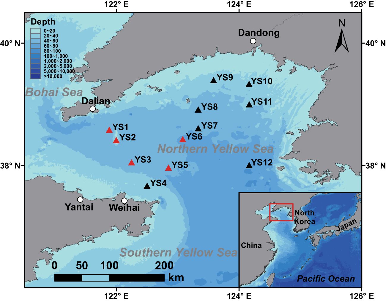
Figure 1. Distribution of sampling sites in the northern Yellow Sea (NYS). The sites marked in red are located in the CWMR and those marked in black are located in the OR.

The collections of in-situ physical parameters, biological samples, and chemical samples were carried out simultaneously on the same voyage every summer. Temperature, salinity, depth, and pH were determined with a SeaBird CTD system (SeaBird, USA), while water samples from various depths were collected using multi-bottled water samplers. Dissolved oxygen (DO) was determined by iodometric titration according to the National Standard of China (GB/T 17378.4-2007). A subsample (500 mL) from each depth layer was filtered through a 0.7 μm GF/F filter (Whatman, UK) using a vacuum of no more than 50 kPa for subsequent analysis of chlorophyll a (Chl-a). The filtered seawater was transferred to a 100 mL polyethylene terephthalate bottle and frozen at -20°C for subsequent nutrient analysis. Phytoplankton samples were collected by towing a plankton net (76 μm mesh size, 37 cm mouth diameter) vertically from a depth of 2 m above the seafloor to the surface at a speed of 0.5 m/s. The volume of filtered water was calculated by multiplying the rope length by the mouth area of the net (Wang et al., 2024). These samples were then preserved in 1 L polyethylene bottles with formaldehyde (final concentration 5%) for subsequent analysis, specifically targeting micro-phytoplankton species. Zooplankton samples were collected using two different mesh sizes of plankton nets (net I: 505 μm mesh size, 50 cm mouth diameter; net II: 160 μm mesh size, 32 cm mouth diameter), fixed with formaldehyde (final concentration 5%), and stored in 500 mL polyethylene bottles. The volume of filtered water was calculated in the same way as for phytoplankton. Sampling of plankton was performed according to the National Standard of China (GB/T 12763.6-2007).

2.2 Chemical and biological measurements

Chl-a was extracted in 5 mL of 90% acetone in the dark for 24 h at 4°C, and a fluorometer (Turner Designs, USA) was used for measuring fluorescence (Welschmeyer, 1994). Dissolved inorganic nitrogen (DIN: NO₃^–N, NO₂^–N, and NH₄⁺-N), dissolved inorganic phosphorus (DIP: PO₄^3–-P), and dissolved silicate (DSi: SiO₃^2–-Si) were measured using a continuous flow analyzer (AA3, Seal Analytical, Germany). The element (N/P, N/Si, and Si/P) ratios were the ratios of the molar concentrations of elements. Phytoplankton samples were identified and counted using an Olympus CX31 microscope (Olympus, Tokyo, Japan) following the Utermöhl method (Utermöhl, 1958). Each species was identified to the lowest possible taxonomic level and the validity of taxonomic names was checked on the AlgaeBase website (http://www.algaebase.org). Zooplankton samples were identified and counted under a dissecting microscope (Leica, Germany). The phytoplankton or zooplankton abundance was obtained by dividing the number of phytoplankton cells or zooplankton individuals by the volume of filtered water.

2.3 Physicochemical indices and criteria

The vertical mean temperature gradient (hereinafter referred to as gradient) was calculated by Equation 1 to characterize the thermocline intensity (Zhou et al., 2009):

$\begin{array}{ll}\text{Gradient }=(T_{\text{b}}-T_{\text{s}})⁄D_{max}& (1)\end{array}$

where T_b is bottom temperature; T_s is surface temperature; D_max is maximum depth, i.e., water column depth.

The depth-averaged value (V_d) of the physicochemical factors was calculated using Equation 2:

$\begin{array}{ll}{V}_{\text{d}}=\frac{1}{D_{max}}{\displaystyle {\sum }_{i=1}^{n-1}\frac{V_i+V_{i+1}}{2}(D_{i+1}-D_i)}& (2)\end{array}$

where D_max is as defined above; n is the maximum number of sampling layers; V_i is the value in the ith sampling layer; D_i is the depth of the ith water layer.

The average Niño3.4 index (https://psl.noaa.gov/data/climateindices/list/) for the previous winter (December-February) was used as an index for the El Niño-Southern Oscillation (ENSO).

Nutrient limitations were determined following the minimum thresholds for phytoplankton growth (also known as absolute limitation) and stoichiometry ratios (also known as potential limitation), respectively (Yin et al., 2013). DIN concentrations of <1 μM, DIP concentrations of <0.1 μM, and DSi concentrations of <2 μM were considered limiting to phytoplankton growth. Stoichiometric limitations were determined with atomic ratios as follows: N/P<10 and N/Si<1 for nitrogen (N) limitation; N/P>22 and Si/P>22 for phosphorus (P) limitation; and N/Si>1 and Si/P<10 for silicon (Si) limitation. Due to the absence of DSi data, the summers of 2011-2013 were exceptional, with N/P<10 for N limitation and N/P>22 for P limitation (Song et al., 2020).

2.4 Biological indices

The diversity indices, including Margalef’s richness (D) (Margalef, 1968), Shannon-Weiner diversity (H′) (Shannon and Weaver, 1949), and Pielou’s evenness (J) (Pielou, 1969), were calculated for each sample using the vegan package according to Equations 3–5.

$\begin{array}{ll}D=(S-1)/{\text{log}}_{2}N& (3)\end{array}$

$\begin{array}{ll}{H}^{\prime }={\displaystyle {\sum }_{i=1}^S(n_i/N){\text{log}}_2(n_i/N)}& (4)\end{array}$

$\begin{array}{ll}J=\frac{H\text{'}}{{\text{log}}_{2}S}& (5)\end{array}$

where S is total number of species in the sample; N is total number of individuals in the sample; n_i is abundance of the ith species in the sample.

The dominance (Yi) of phytoplankton species/genus for each summer was calculated according to Equation 6, and species/genera with Yi ≥ 0.02 were considered dominant in the studied area (Sun et al., 2004).

$\begin{array}{ll}{Y}_i=\frac{n_i}{N}{f}_i& (6)\end{array}$

where n_i and N are the same as above; f_i is ratio of the number of sites where the ith species appear to the total number of sites.

The Dia/Dino index for each sample was calculated by Equation 7 (Mokrane et al., 2019):

$\begin{array}{ll}\text{Dia}/\text{Dino index}=A{b}_{\text{Dia}}/(A{b}_{\text{Dia}}+A{b}_{\text{Dino}})& (7)\end{array}$

where Ab_Dia is diatom abundance; Ab_Dino is dinoflagellate abundance.

2.5 Statistical analysis

Locally weighted least squares (Loess) regression was conducted with R (R Core Team, 2018) to determine the dynamic trends of environmental variables as well as the relationship between the phytoplankton and environmental variables. Multiple comparisons of phytoplankton abundance and diversity indices among years were conducted using R. Shapiro-Wilk and Levene’s tests were performed using the stats and car packages respectively to assess the normality and homogeneity of variance. Kruskal-Wallis test with posthoc Nemenyi test was employed using the stats package and PMCMRplus packages since the data were non-normally distributed. Mann-Whitney U test was performed to compare environmental factors and dominant species between different regions. Statistical significance was set at p < 0.05 for hypothesis testing of differences.

The depth-averaged environmental variables were used to investigate the correlation between phytoplankton and environmental factors. Their relationship was also explored using constrained ordinations, based on square-root transformed abundance data and log₁₀(x+1) transformed environmental data except for pH data. The missing values of environmental factors were replaced by the overall means. Firstly, detrended correspondence analysis (DCA) was conducted on the biological data and the type of canonical ordination methods was selected according to the length of the first DCA axis. The unimodal model (canonical correspondence analysis, CCA) was used when the length of the first DCA axis length was > 4, and the linear model (redundancy analysis, RDA) was used when the length was < 3 (Lepš and Šmilauer, 2003). Then, variables with variance inflation factors (VIF) > 10 were removed from the ordination analysis to avoid high collinearity. Forward selection was carried out using the packfor package to identify statistically significant explanatory variables. Spearman correlations between phytoplankton taxa and diversity indices and between phytoplankton taxa/diversity and environmental factors were calculated with the Hmisc package. Spearman correlation analysis was also conducted between the site-averaged abundance in August and the Niño3.4 index for the previous winter, in order to explore the relationship between climate change and phytoplankton dynamics.

3 Results

3.1 Variation in environmental factors

3.1.1 Temporal trends in environmental factors

Temperature, gradient and salinity showed an overall upward trend (Figure 2), while pH, DIN concentration, N/P ratio, N/Si ratio (no data from 2011-2013), and Chl-a concentration showed a downward trend (Figure 2). Among them, salinity, pH, DIN, N/P ratio, and Chl-a showed significant differences among years (Kruskal-Wallis test: p < 0.05). DO, PO₄^3–-P, SiO₃^2–-Si, and net I and II zooplankton abundances showed no obvious upward or downward trend (Figure 2). The N/P ratio was particularly high in the summer of 2011 (116.60), while in other years it ranged from 8.79 to 29.19 (Figure 2). The surface temperature rose first and then decreased, reaching the highest in 2018, while the bottom temperature changed little during the study period except for 2019 in which only one site was with a high value (Supplementary Figures S1, S2). The salinity in both the surface and bottom layers showed an upward trend. The DIN concentration at the surface was the highest in 2011 and changed little in the summers of 2012-2020, while the DIN concentration at the bottom showed an overall downward trend, reaching the highest in 2011 and was also high in 2014 (Supplementary Figures S1, S2). The PO₄^3–-P concentration at the surface reached the highest in 2014, and that at the bottom reached the highest in 2014 and the lowest in 2011 (Supplementary Figures S1, S2). The SiO₃^2–-Si concentration at the surface did not show a clear trend but was higher in 2018 and 2019, while the SiO₃^2–-Si concentration at the bottom showed a slight downward trend and reached the lowest in 2019 (Supplementary Figures S1, S2). The N/P ratio, like DIN concentration, was the highest in the surface and bottom layers in 2011 and changed little in the other nine years (Supplementary Figures S1, S2). The N/Si ratio changed little at the surface and was lower at the bottom in 2017 and 2020, while the Si/P ratio changed little in both the surface and bottom waters (Supplementary Figures S1, S2).

Figure 2

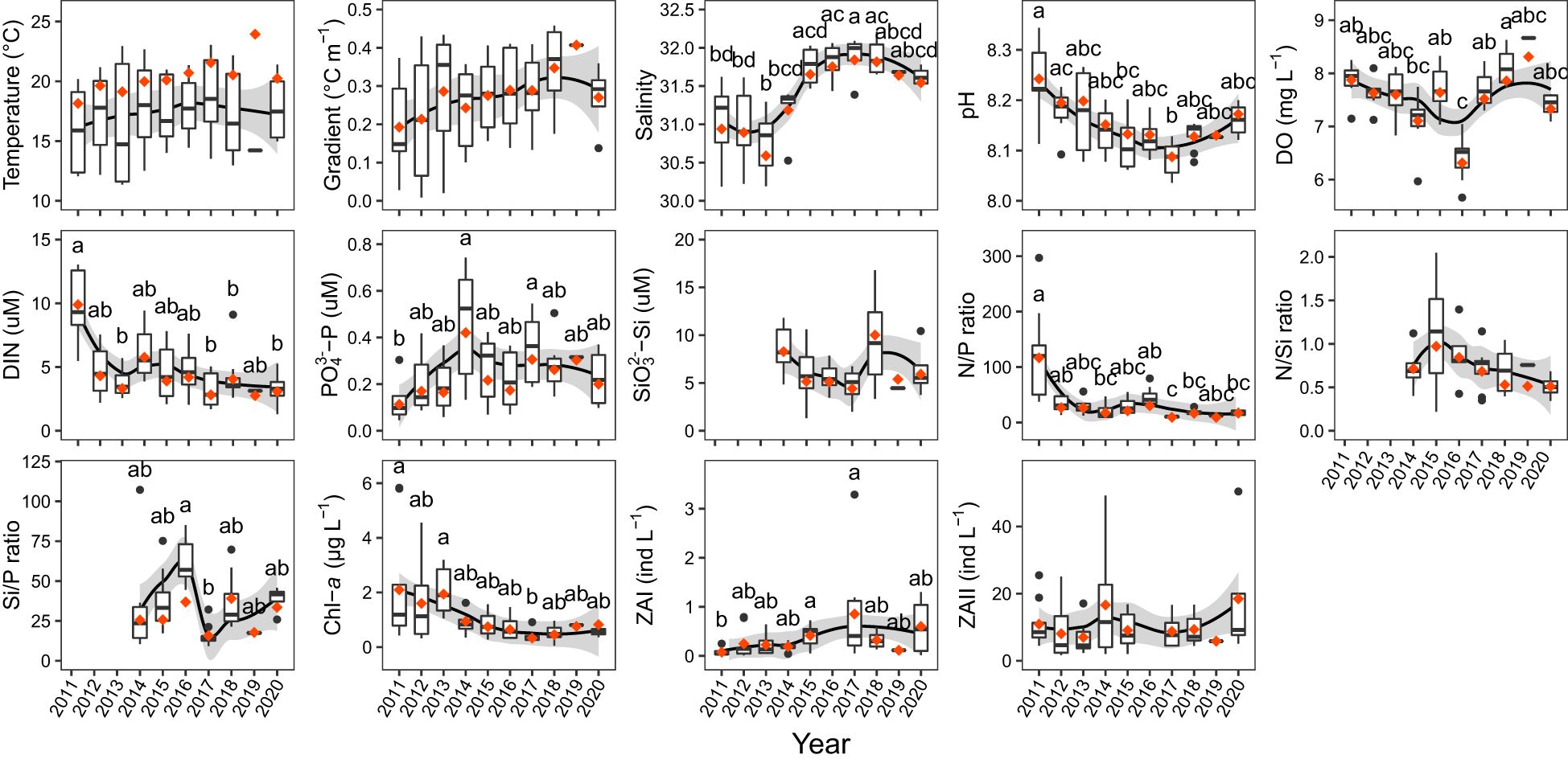
Figure 2. Temporal trends in environmental factors in the NYS in summer. The depth-averaged values are shown. The black line is the LOESS regression line, and the gray shadow is the 95% confidence interval. The orange diamond dots represent the average values, and the black circle dots represent the outliers. The letters above bars indicate differences between years, and the absence of the same letters indicates a significant difference (Nemenyi test: p < 0.05). A lack of letter marks indicates no significant difference among years (Kruskal-Wallis test: p ≥ 0.05). ZAI, net I zooplankton abundance; ZAII, net II zooplankton abundance.

3.1.2 Difference in environmental factors between the CWMR and OR

There were no significant differences in environmental factors in the surface waters between the CWMR and OR, except for temperature, which was significantly higher in the CWMR (Figure 3). In contrast, the environmental factors in the bottom waters exhibited considerable differences between the two regions (Figure 3). Specifically, the bottom waters in the CWMR displayed lower levels of temperature, pH, N/P ratio, Si/P ratio, and Chl-a concentration, while showing higher levels of salinity, DO, DIN, PO₄^3–-P, and SiO₃^2–-Si compared to the OR (Figure 3). Additionally, the gradient was significantly greater in the CWMR than that in the OR (Figure 3). The gradient in the CWMR did not demonstrate a clear temporal trend (Supplementary Figure S3), although both surface and bottom temperatures in this region showed an upward trend (Supplementary Figures S4, S5). In contrast, the gradient in the OR showed an increasing trend (Supplementary Figure S6), as the surface temperature in this region increased while the bottom temperature changed little (Supplementary Figures S7, S8). Overall, temporal trends in other environmental factors differed little between the two regions (Supplementary Figures S3–S8).

Figure 3

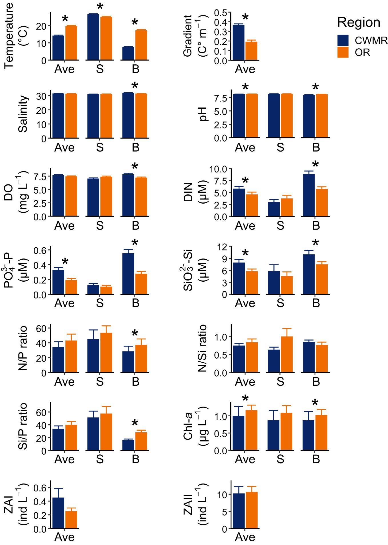
Figure 3. Comparison of environmental factors between the CWMR and OR. An asterisk indicates a significant difference between the regions (Mann-Whitney U test: p < 0.05). Ave, depth-averaged; S, surface; B, bottom.

3.1.3 Nutrient limitation for phytoplankton

DIN, PO₄^3–-P, and SiO₃^2–-Si concentrations were higher in the middle and bottom waters than in the surface and subsurface at most of the sites (Supplementary Figure S9). DIN concentrations that limit phytoplankton growth (< 1 μM) were found at the surface of several sites in 2012, 2013, 2015 and 2020 (Supplementary Table S2). PO₄^3–-P concentrations that limit phytoplankton growth (< 0.1 μM) existed at the surface of several sites in most years (2011-2016, 2018, 2020), and also existed at the bottom of several sites in 2011, 2013, 2016 (Supplementary Table S2). SiO₃^2–-Si concentrations that limit phytoplankton growth (< 2 μM) occurred at the surface of one site and at the bottom of several sites in 2015, as well as at the surface of several sites in 2016 and 2017 (Supplementary Table S2). In terms of absolute limitations of nutrients for phytoplankton growth, P limitation was more common than N and Si limitations in the NYS, and was more severe in the surface waters (Figure 4). Potential N limitation existed at the bottom layer of one site in 2013 and the surface and bottom layers of several sites in 2017-2020 (Supplementary Table S2). Potential P limitation existed at both the surface and bottom layers of several sites in 2011-2014, 2016, 2018, and 2020, and at the surface layer of several sites in 2015 (Supplementary Table S2). Potential Si limitation was only recorded at the bottom of one site in 2015 (Supplementary Table S2). Considering the potential limitations, P limitation persistently existed in the NYS, while N limitation became more common from 2017 to 2020 (Figure 4). Both the absolute and potential P limitations were slightly less severe in the CWMR than in the OR (Supplementary Table S3).

Figure 4

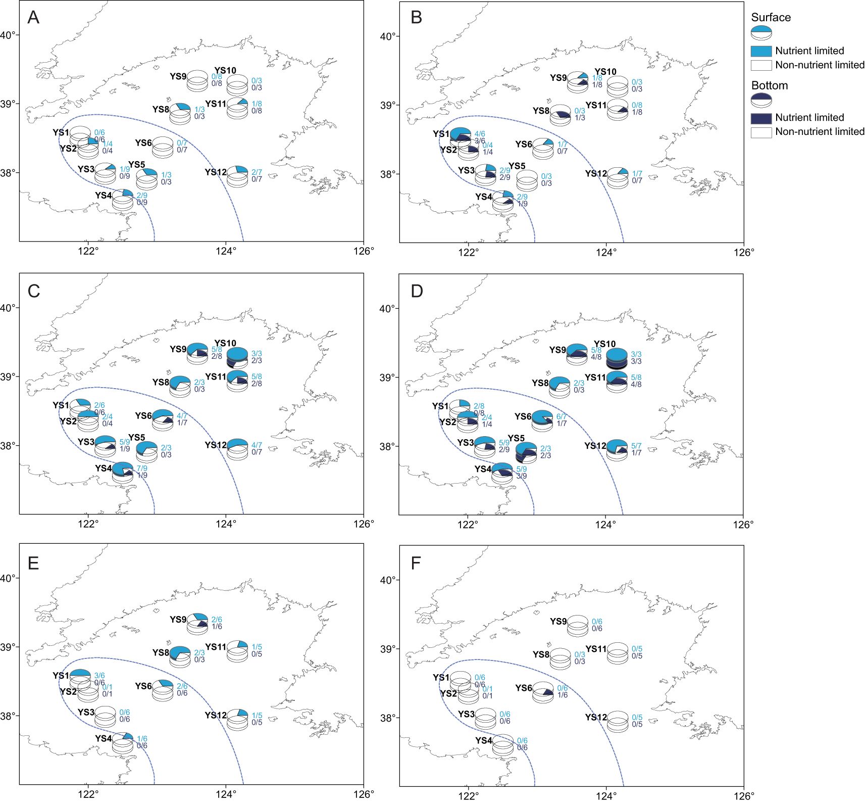
Figure 4. Spatial distribution of frequency of nutrient limitation in the NYS in summer. (A) DIN concentration limitation, (B) Potential DIN limitation, (C) DIP concentration limitation, (D) Potential DIP limitation, (E) DSi concentration limitation, (F) Potential DSi limitation. The proportion of colored parts in the pie represents the ratio of the number of years of nutrient limitation to the total number of years of sampling. The area surrounded by the blue dashed line is the approximate area occupied by the YSCWM.

3.2 Variation in phytoplankton communities

3.2.1 Community composition and abundance

A total of 109 phytoplankton taxa (including unidentified species) were identified, belonging to Bacillariophyta (81 species, 39 genera), Dinoflagellata (27 species, 7 genera), and Ochrophyta (1 species, 1 genera) (Supplementary Table S4). Chaetoceros (20 species), Coscinodiscus (11 species), Protoperidinium (11 species), and Tripos (10 species) were the genera with the maximum number of observed species.

The average abundance of total phytoplankton across the whole study area reached its highest level in 2011 (1527 cells L^-1), followed by relatively high levels in 2017 (1331 cells L^-1) and 2015 (1204 cells L^-1), and the lowest average abundances were recorded in 2012 (95 cells L^-1), 2013 (100 cells L^-1), and 2014 (102 cells L^-1) (Figure 5A). Bacillariophyta abundance peaked in 2011 (1504 cells L^-1), with relatively high levels in 2015 (1125 cells L^-1) and 2017 (962 cells L^-1) and the lowest Bacillariophyta abundance was observed in 2014 (18 cells L^-1) (Figure 5A). Both total abundance and Bacillariophyta abundance showed high values at site YS9 which is close to the southern part of Liaodong Peninsula, in the summers of 2011, 2015 and 2017, especially in 2011, causing the mean total abundance and mean Bacillariophyta abundance higher in these years (Figure 5B; Supplementary Figure S10). Dinoflagellata abundance reached its highest level in 2017 (369 cells L^-1), with higher values in the Bohai Strait and the southern part of Liaodong Peninsula, while the lowest Dinoflagellata abundance occurred in 2011 (23 cells L^-1) (Figure 5A; Supplementary Figure S11). The abundance of Ochrophyta was highest in 2020 (1 cells L^-1) and was as low as 0 cells L^-1 in 2019 when sampling was conducted at only one site (Figure 5A). The Dia/Dino index was highest in 2011 (0.75), followed by 2015 (0.61), and the lowest ratio were recorded in 2019 (0.21) and 2014 (0.24) (Figure 5A).

Figure 5

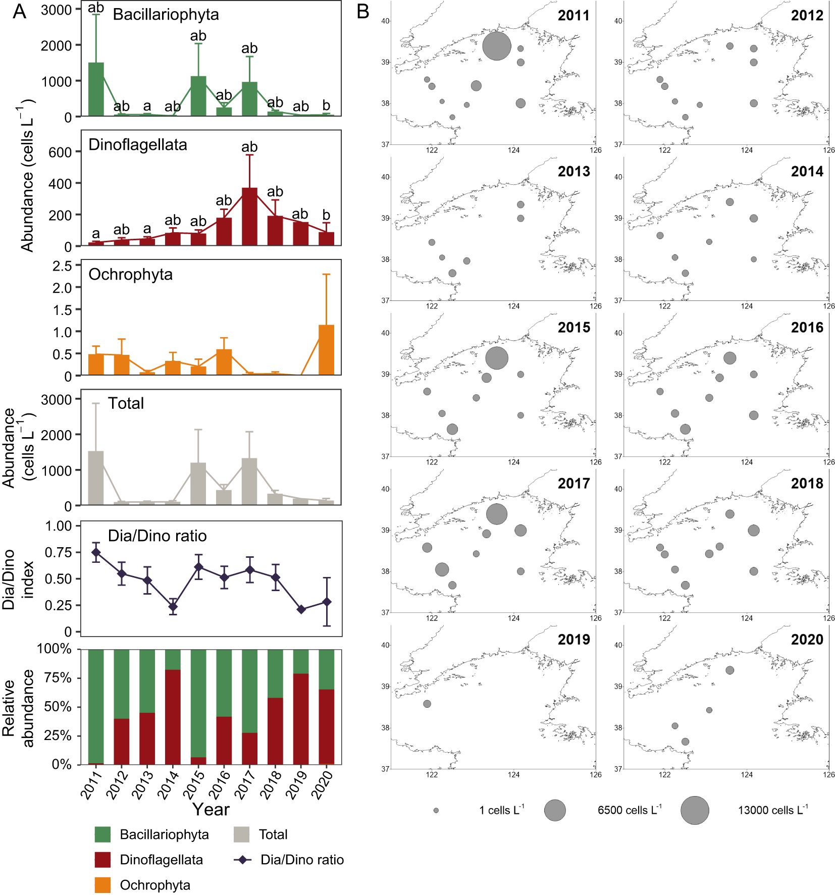
Figure 5. Phytoplankton abundance in the NYS in summer. (A) Trends in phytoplankton abundance. Bars and error bars represent means and standard errors. Multiple comparisons (Kruskal-Wallis test) are performed among years for both absolute abundances and the Dia/Dino index. The letters above bars indicate differences between years and the absence of the same letters indicates a significant difference (Nemenyi test: p < 0.05). A lack of letter marks indicates no significant difference among years (Kruskal-Wallis test: p ≥ 0.05). (B) Distribution of the total phytoplankton abundance.

3.2.2 Dominant taxa

Seven genera were dominant in at least one summer during the study period, they were Chaetoceros, Tripos, Proboscia, Paralia, Coscinodiscus, Noctiluca, and Pyrophacus. Among them, Tripos and Paralia showed significant differences in abundance among different years, while the abundances of the other five genera did not differ significantly (Figure 6A). The abundance of Tripos was significantly higher in 2016 and 2017 compared to 2011 and 2012 (Figure 6A). The abundance of Paralia was significantly higher in 2017 compared to 2014 (Figure 6A). The abundance of Pyrophacus in 2015 was significantly higher than that in 2011, 2017 and 2020, and the abundance in 2012 was significantly higher than that in 2011 and 2017 (Figure 6A). As many as 33 dominant species were recorded in at least one summer during 2011-2020 (Figures 6B, C). The number of dominant species each summer ranges from 3 to 15 (Figure 6C). Paralia sulcata and Tripos muelleri remained dominant throughout the study period (Figure 6B; Supplementary Figure S12, S13). Tripos fusus, Noctiluca scintillans, and Pyrophacus steinii also appeared as dominant species with relatively high frequency (Figure 6B).

Figure 6

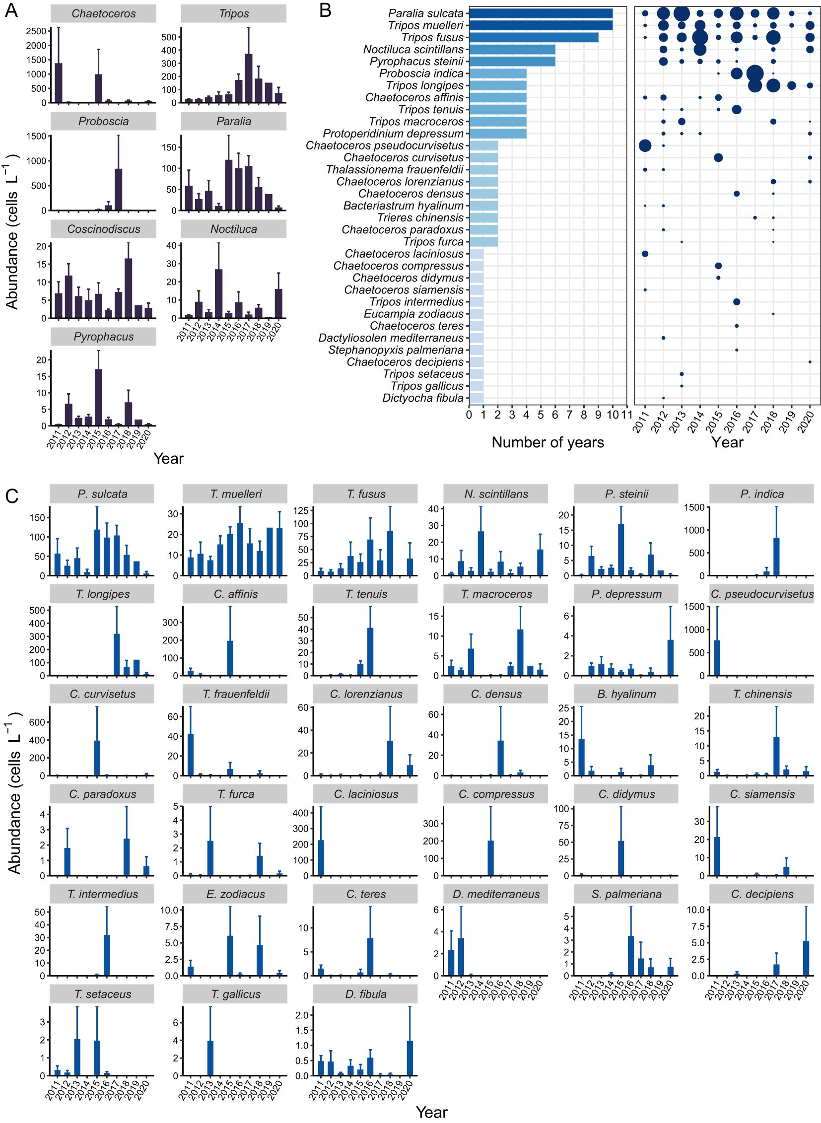
Figure 6. Dominant phytoplankton taxa in the NYS in summer. (A) Abundance of the dominant genera. (B) Frequency (number of years) and dominance of the dominant species. The point size is proportional to the value of the dominance index. (C) Abundance of the dominant species. In panels (A, C), bars and error bars represent means and standard errors.

3.2.3 Diversity

The diversity indices, including total species number (S), Margalef’s richness (D), Shannon diversity (H’), and Pielou’s evenness (J) fluctuated slightly in the summers of 2011-2020, but the differences among years were not statistically significant and there was no clear trend in these indices (p ≥ 0.05) (Figure 7A). S and D were positively correlated with the relative abundance of Bacillariophyta, the absolute/relative abundances of Chaetoceros and Proboscia, and the Dia/Dino index, while they were negatively correlated with the relative abundances of Dinoflagellata and Tripos (Figure 7B). J was negatively correlated with the total phytoplankton abundance, the absolute/relative abundances of Bacillariophyta and Paralia sulcata, and the Dia/Dino index (Figure 7B).

Figure 7

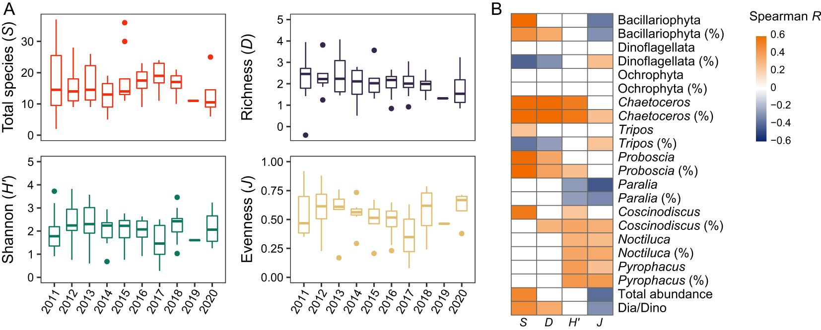
Figure 7. Diversity indices of the phytoplankton communities in the NYS in summer. (A) Temporal trends in diversity indices. No significant difference is detected in each diversity index among years (Kruskal-Wallis test: p ≥ 0.5). (B) Spearman heatmap showing the correlations between the diversity indices and the environmental factors. Names of taxa with or without “%” in parentheses denote relative and absolute abundances, respectively. Blank cells represent nonsignificant correlations (p ≥ 0.5).

3.3 Relationship between phytoplankton community and environment

3.3.1 Relationship between community variations and environment factors

The relationship between the absolute/relative abundances of species/phyla and the environmental factors was analyzed using RDA. The variable N/P ratio was removed from the ordination analyses to ensure that the VIFs for all remaining variables were less than 10. The variation in the absolute abundance of species was significantly correlated with DO (Figure 8A), while the variation in the relative abundance of species was significantly correlated with net II zooplankton abundance (Figure 8B). The variation in the absolute abundance of phyla was significantly correlated with DO (Figure 8C), while the variation in the relative abundance of phyla was significantly correlated with both DO and net II zooplankton abundance (Figure 8D).

Figure 8

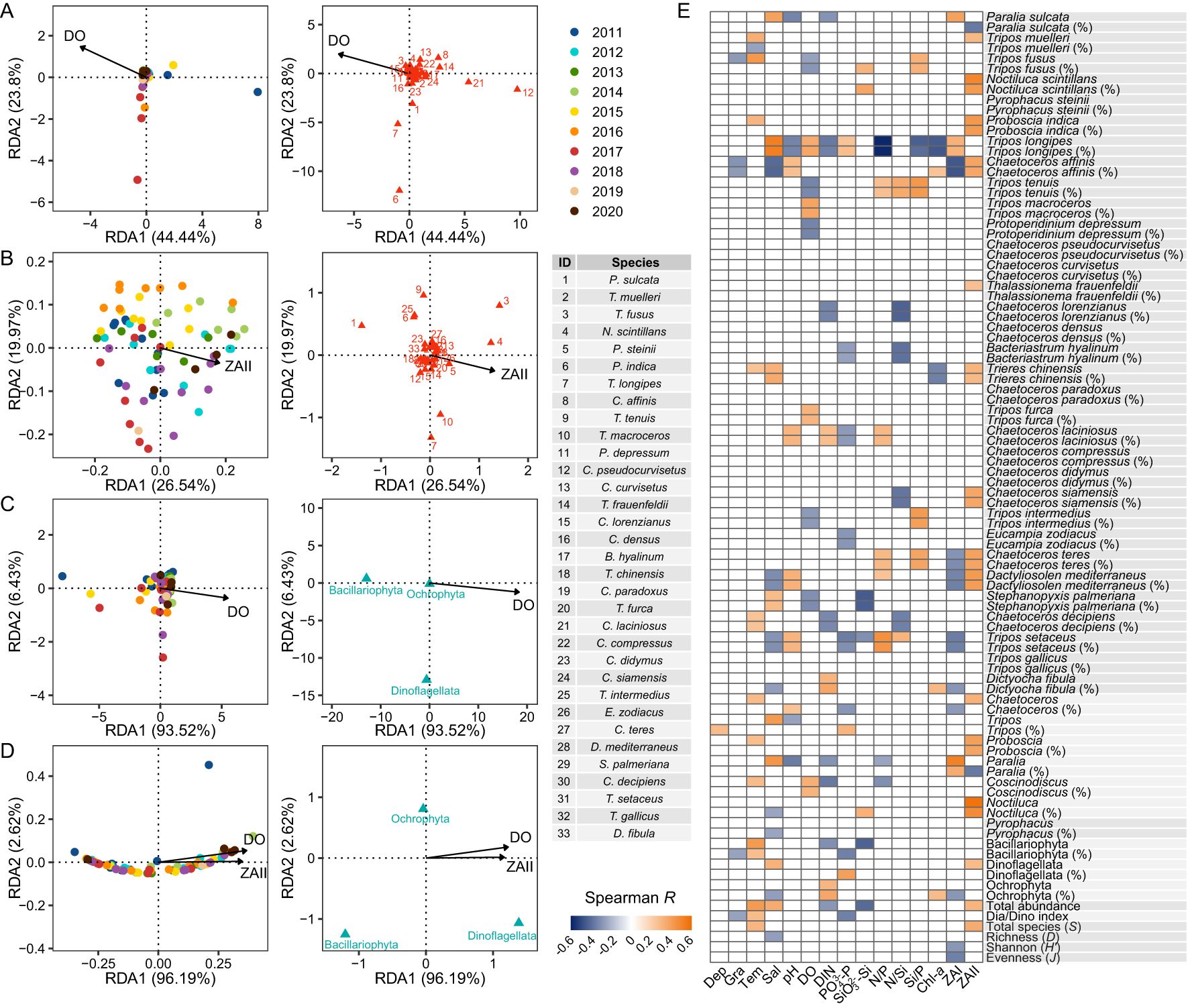
Figure 8. Relationship between the phytoplankton community structure and environmental factors in the NYS in summer. The ordination biplots show the relationships between (A) the absolute abundance of species/ (B) the relative abundance of species/ (C) the absolute abundance of phyla/ (D) the relative abundance of phyla and the environmental factors. (E) Spearman correlations between the phytoplankton abundances/diversity indices and the environmental factors. Names of taxa with or without “%” in parentheses denote relative and absolute abundances, respectively. Blank cells represent nonsignificant correlations (p ≥ 0.5). Dep, depth; Gra, gradient; Tem, temperature; Sal, salinity. See the caption of Figure 2 for other abbreviations.

Spearman analysis showed that the total phytoplankton abundance, absolute/relative abundances of Bacillariophyta, Dia/Dino index, and total species number (S) were positively correlated with temperature (Figure 8E). The relative abundance of Bacillariophyta and Dia/Dino index were negatively correlated with gradient and PO₄^3–-P, while the relative abundance of Dinoflagellata was positively correlated with these environmental variables (Figure 8E). The Shannon diversity and evenness were negatively correlated with net I zooplankton abundance (Figure 8E). The absolute abundance of P. sulcata had a positive correlation with salinity and net I zooplankton abundance, and a negative correlation with pH and DIN (Figure 8E). The absolute abundance of T. muelleri was positively correlated with temperature and net I zooplankton abundance (Figure 8E), whereas its relative abundance was negatively correlated with temperature. The absolute/relative abundances of Tripos longipes had strong correlations with multiple environmental factors, including a positive correlation with salinity, DO, PO₄^3–-P, and net I zooplankton abundance, and a negative correlation with N/P ratio, Chl-a, Si/P ratio, DIN, and pH (Figure 8E).

3.3.2 Relationship between community variations and the YSCWM

The average abundance of Bacillariophyta (868 cells L^-1) was much higher than that of Dinoflagellata (130 cells L^-1) in the OR, while the average abundance of Dinoflagellata (116 cells L^-1) exceeded that of Bacillariophyta (75 cells L^-1) in the CWMR (Figure 9A). According to the results of Mann-Whitney U test, the total phytoplankton abundance, the absolute/relative abundances of Bacillariophyta, the Dia/Dino index, and total species number (S) were significantly lower in the CWMR than in the OR (Figures 9A, B, G). Among the dominant genera and species, the absolute/relative abundances of Chaetoceros and Chaetoceros compressus, as well as the absolute abundances of Coscinodiscus and T. fusus, were significantly lower in the CWMR compared to the OR (Figures 9C–F). Only T. muelleri exhibited a significantly higher relative abundance in the CWMR than in the OR, but no significant difference was observed in its absolute abundance (Figures 9E, F).

Figure 9

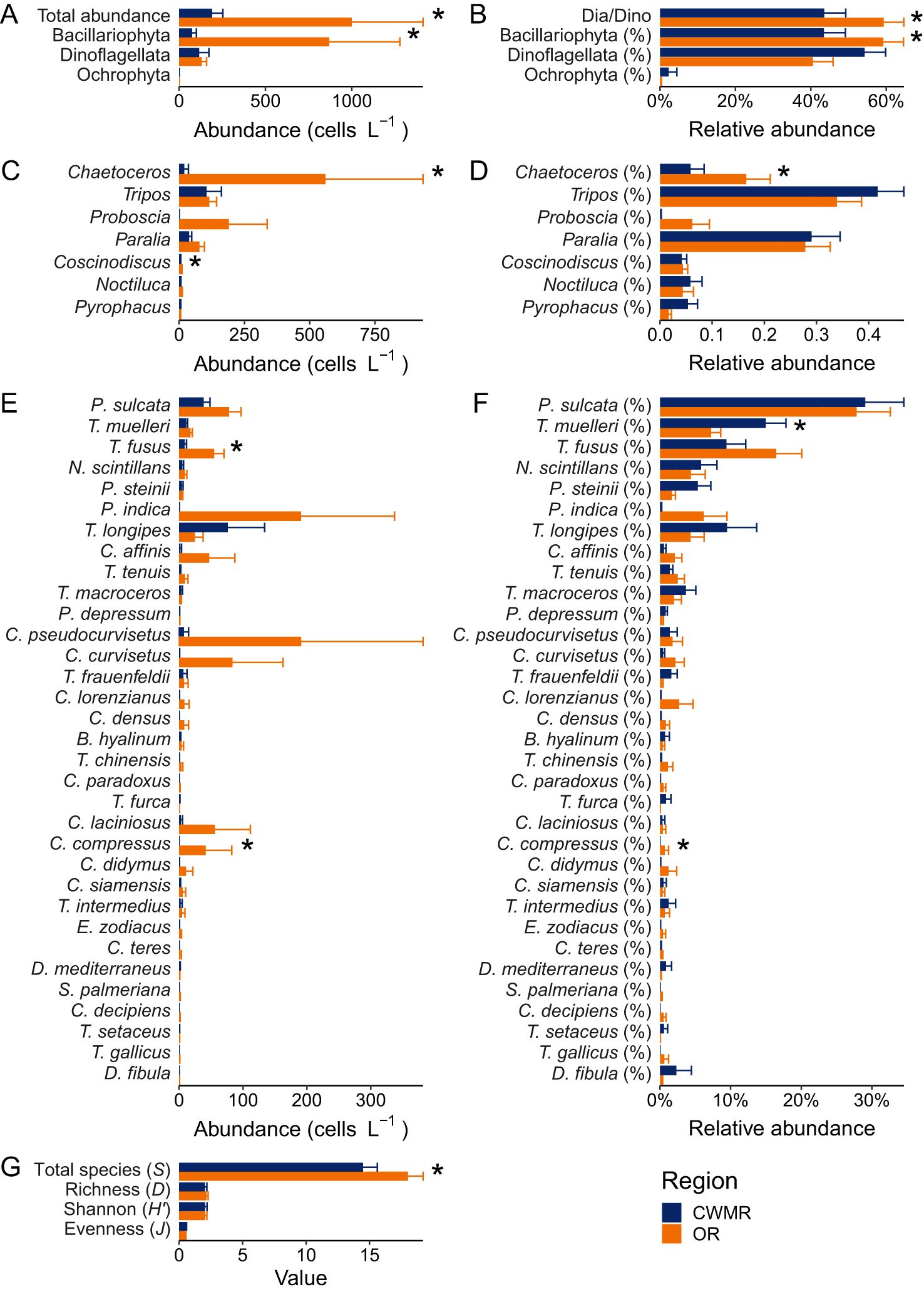
Figure 9. Comparison of phytoplankton abundance and diversity between the CWMR and OR. (A) Absolute abundances of total phytoplankton and three major phyla. (B) The Dia/Dino index and relative abundances of three phyla. (C) Absolute abundances of dominant genera. (D) Relative abundances of dominant genera. (E) Absolute abundances of dominant species. (F) Relative abundances of dominant species. (G) Diversity indices. In panels (A–G), an asterisk indicates a significant difference between the regions (Mann-Whitney U test: p < 0.05). Names of taxa with or without “%” in parentheses denote relative and absolute abundances, respectively.

3.3.3 Relationship between community variations and ENSO

The mean Niño3.4 index for the previous winter showed no significant correlation with the absolute/relative abundances of Bacillariophyta, Dinoflagellata, Ochrophyta, or the Dia/Dino index (p ≥ 0.5), but it showed significant correlations with the abundances of some dominant genera or species (Figure 10). It was negatively correlated with the absolute/relative abundances of Coscinodiscus, Thalassionema frauenfeldii, Bacteriastrum hyalinum, Tripos furca, Dactyliosolen mediterraneus and the relative abundance of Tripos macroceros (Figure 10; Supplementary Table S5). A significantly positive correlation was only detected between the index and the absolute abundance of T. muelleri (Figure 10; Supplementary Table S5).

Figure 10

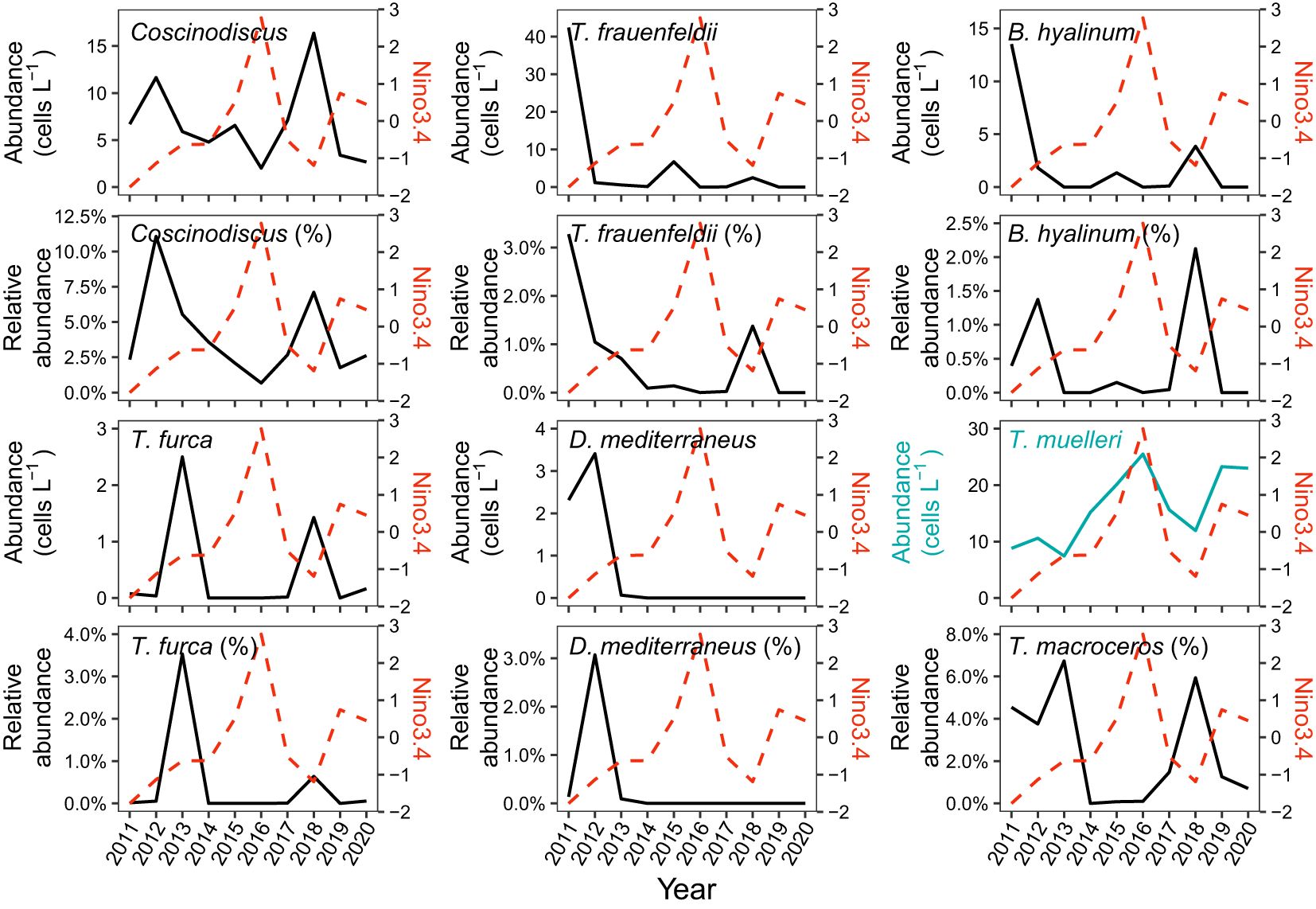
Figure 10. Relationship between the absolute/relative abundances of dominant genus/species and the Niño3.4 index for last winter. Only significant correlations (p < 0.05) are shown. Names of taxa with or without “%” in parentheses denote relative and absolute abundances, respectively. The cyan and black lines depict the abundances of taxa positively and negatively correlated with the Niño3.4 index, respectively.

4 Discussion

4.1 Associations between environmental changes and phytoplankton community shifts in the NYS

During the study period, several environmental factors in the NYS during summer showed clear temporal trends. The depth-averaged temperature in 2017 was 2.8°C higher than in 2011. Numerous surveys indicated a long-term rising trend in temperature within the NYS (Li et al., 2022; Park et al., 2015; Pei et al., 2017). However, the upward trend observed during the study period was even more pronounced, aligning with the characteristics noted by Li et al. (2022) for the period from 2011 to 2017. The temperature gradient also exhibited a general upward trend. In the CWMR, the gradient changed little due to the simultaneous rise in both surface and bottom temperatures. In contrast, the gradient in the OR tended to rise as the temperature difference between the surface and bottom increased. Additionally, salinity showed an obvious upward trend during the study period, continuing the long-term increase in salinity observed from the mid-20^th century to the early 21^st century (Ma et al., 2006; Lv, 2008). Previous studies attributed this long-term increase in salinity to the growing disparity between evaporation and precipitation, as well as the reduction of freshwater influx into the NYS (Ma et al., 2006; Lv, 2008). Collectively, the long-term trends in temperature, gradient, and salinity in the NYS were related to global climate change.

The nutrient structure in the NYS also underwent drastic changes during the study period. Notably, the DIN concentration and N/P ratio peaked in the summer of 2011, followed by a marked decline and stabilization in the following years. This shift was primarily due to stringent anthropogenic nitrogen emission regulations implemented by the Chinese government in the early 2010s, which led to a reduction of DIN levels in the NYS, which was predominantly sourced from river inputs and rainfall, thereby reversing a previously continuous upward trend (Yu et al., 2019; Zheng and Zhai, 2021). The nutrient structure in the NYS, particularly the N/P ratio, decreased along with the change in DIN level. In addition, the Chl-a concentration, a proxy for phytoplankton biomass, exhibited a significant decline after reaching its highest levels in the summers of 2011 and 2013, ultimately hitting a low in the summer of 2017. Given that the temporal trends in Chl-a concentration mirrored those of DIN and the N/P ratio, it was presumed that these changes in nutrient levels and structure were primary drivers of the observed variations in Chl-a. A recent study have indicated that enhanced summer stratification in the NYS, which restricted the upward turbulent diffusion of deep waters rich in nutrients and Chl-a, also contributed to the decline in Chl-a concentration (Zhai et al., 2023). Additionally, a downward trend in pH was observed in the summers of 2011 to 2017, followed by a rebound in the summers after 2017. Li et al. (2022) reported a significant decrease in pH in the NYS over a 40-year period (1976-2017), particularly during summer, attributing this decline to increased net respiration in biomes due to eutrophication. In this study, pH exhibited a positive correlation with Chl-a, showing a marked decrease initially, followed by a slight increase after 2017. Therefore, the overall decrease in pH was less likely to be linked to an increase in total phytoplankton biomass and community net respiration. However, the abundances of net I zooplankton and certain dominant phytoplankton species, such as Paralia sulcata and Tripos longipes, were significantly and negatively correlated with pH. This suggested that a decline in pH might be associated with an increase in the biomass of these dominant species and macro/mesozooplankton, and vice versa.

The abundances of the total phytoplankton, Bacillariophyta and Dinoflagellata, the Dia/Dino index, and the diversity indices in the NYS showed no significant increasing or decreasing trend during the study period. Bacillariophyta and Dinoflagellata were the main phytoplankton phyla, and their relative dominances varied greatly, with Bacillariophyta dominating in the summers of 2011 and 2015, and Dinoflagellata dominating in 2014 and 2019. This result was consistent with previous surveys that the dominant groups were not consistent in the summertime of different years (Zhang et al., 2014; Hou et al., 2021; Fu, 2021). Additionally, some previous surveys based on multilayer sampling have indicated that the vertical distribution patterns of dominant groups also varied among different years. Zhang et al. (2014) reported that Dinoflagellata dominated in the phytoplankton communities in the NYS in June 2011, with Prorocentrum minimum being the primary dominant species; Dinoflagellata, similar to the total phytoplankton, exhibited a higher abundance in the upper waters (20m depth), whereas Bacillariophyta, primarily consisting of P. sulcata, showed a higher abundance in the bottom waters. Hou et al. (2021) found that in June and July of 2013, Bacillariophyta dominated in the phytoplankton communities in the NYS and the phytoplankton abundance was higher in the middle and bottom layers. The most important dominant species were P. minimum, Cylindrotheca closterium, P. sulcata and Thalassiosira sp. According to the observations of Lv et al. (2016), Bacillariophyta was dominant in phytoplankton communities in the cold water mass region in the NYS in August 2014, and the main dominant species were Thalassiosira sp. and Thalassiosira pacifica. High values of the total phytoplankton abundance and Chl-a concentration occurred from the subsurface (20m depth) to the bottom. Fu (2021) reported that Bacillariophyta was the dominant group in the NYS in July and August of 2020, and P. sulcata was the first dominant species. The abundances of total phytoplankton and Bacillariophyta did not change significantly with depth, but the abundances of Dinoflagellata were higher at the surface and bottom than in the middle layer.

Whether diatoms or dinoflagellates dominated the phytoplankton community often depends on the interaction of multiple environmental factors and is of great concern in the context of climate change and increased eutrophication (Bi et al., 2021). Therefore, we tried to explain what factors controlled the relative dominance of diatoms and dinoflagellates in the phytoplankton communities in the NYS. Our research showed that the DIN concentration and N/P ratio were the highest in the summer of 2011, and the Dia/Dino index was also the highest in 2011. This result was inconsistent with most studies, which indicate that an increase in the N/P ratio tends to increase the dominance of dinoflagellates (Glibert et al., 2011; Xiao et al., 2018). The high diatom abundance in 2011 was mainly due to the high diatom (primarily Chaetoceros pseudocurvisetus) abundance at the nearshore site YS9, and similar situations also occurred at the site YS9 in the summers of 2015 and 2017 (primarily Chaetoceros curvisetus and Proboscia indica, respectively). The DIN level in the surface layer of site YS9 was higher in 2011 (14.47 μM), and the N/P ratio was higher in 2011 and 2015 (2011: 213.63, 2015: 94.97). The elevated concentrations of DIN in this region were primarily attributed to inputs from coastal rivers, which facilitated the prolific growth and reproduction of diatoms. We hypothesized that the elevated levels of nutrients imported by coastal rivers were responsible for the extensive growth and proliferation of diatoms in this coastal region. The high N/P ratio can be interpreted as a consequence of phosphorus depletion due to diatom utilization, while nitrogen levels persisted at relatively high concentrations. In contrast, the high diatom abundance at this site in 2017 was likely attributable to increased temperatures and stratification of the water column. This was because the surface temperature at site YS9 was higher and the gradient was stronger than in other years, and P. indica occurred in high abundance at site YS9 with a positive correlation with temperature. These results were consistent with a previous study showing that P. indica has adaptive advantages in high-temperature and stratified environments (Gómez and Souissi, 2007). In summary, our results suggest that the variation in the relative dominance of diatoms and dinoflagellates across different years may be jointly controlled by multiple factors, including nutrient levels and the intensity of water column stratification.

4.2 Impacts of the YSCWM on the phytoplankton communities

The hydrological environment of the NYS is mainly influenced by runoff, coastal currents, seasonal water masses and the Yellow Sea Warm Current, with varying degrees of impact during different periods of the year (Bi et al., 2019; Zhang et al., 2021). The thermocline in the NYS begins to form in spring and reaches its peak strength in summer (August). The YSCWM is the most prominent hydrological phenomenon in the NYS during summer, with its formation, development and weakening nearly coinciding with those of the thermocline. Our data showed that the temperature difference between the surface and bottom waters in the cold center of the YSCWM reached up to 20°C. To assess the effects of the YSCWM on phytoplankton communities, we compared environmental factors and biological indicators between the CWMR and OR.

In terms of environmental features, the CWMR exhibited a stronger gradient compared to the OR. The bottom waters in the CWMR had lower temperatures, pH, N/P and Si/P ratios, and Chl-a levels, while exhibiting higher salinity, DO, and nutrient (DIN, PO₄^3–-P, and SiO₃^2–-Si) concentrations. Regarding biological indices, the total phytoplankton abundance, the absolute/relative abundances of Bacillariophyta, the Dia/Dino index, and species richness (S) were all significantly lower in the CWMR than in the OR. The lower phytoplankton abundance in the CWMR was primarily due to nutrient limitations in the upper waters caused by stratification, which limited the growth of certain phytoplankton taxa. In the CWMR, P limitation was most pronounced in the upper waters, while PO₄^3–-P was generally sufficient in the deep waters. However, the strong stratification prevented the upward transport of nutrients from the deep waters to the surface. The significantly lower diatom abundance and Dia/Dino index in the CWMR could also be largely attributed to the stronger stratification and the distinct nutrient distribution patterns in this region. The vertical migration of dinoflagellates enabled them to access both the deep nutrient pool and near-surface light at different times of the day, giving them a competitive advantage over other phytoplankton groups (Fu et al., 2018; Ji and Franks, 2007; Glibert et al., 2013; Wang et al., 2014). Additionally, the significantly lower phytoplankton species richness (S) in the CWMR was influenced by nutrient distribution patterns caused by stratification, as well as lower temperatures, since phytoplankton diversity is suggested to be positively correlated with temperature within a certain range (Righetti et al., 2019; Segura et al., 2015).

During the study period, the absolute and potential P limitations in the NYS were both significant although the relative P limitation was weakened in the summers of 2017-2020. In comparison, the N and Si limitations were less pronounced than the P limitation. Spearman analysis revealed that the Dia/Dino index was significantly associated with temperature, gradient and PO₄^3–-P concentration. The absolute abundance of Bacillariophyta showed a negative correlation with DIN and SiO₃^2–-Si, while the relative abundance of Bacillariophyta showed a negative correlation with PO₄^3–-P. This was because higher depth-averaged DIN, PO₄^3–-P and SiO₃^2–-Si levels were mainly observed in the CWMR, where the abundances of total phytoplankton and Bacillariophyta were low despite high nutrient levels in the bottom. In contrast to Bacillariophyta, the absolute abundance of Dinoflagellata did not correlate with nutrients while the relative abundance of Dinoflagellata was positively correlated with PO₄^3–-P. This was mainly because the adaptive strategies of dinoflagellates enable them to effectively navigate nutrient limitations in the highly stratified environment in summer. Additionally, RDA indicated that the relative abundance of Bacillariophyta was negatively DO. Such relationship did not indicate a direct impact of DO on phytoplankton groups but was attributable to dominance of dinoflagellates in CWMR compared to the OR and the higher average depth-averaged DO concentration was also higher in the CWMR. The higher DO concentration in the CWMR than the OR in summer was mainly due to the low temperature of the YSCWM, which could increase the solubility of oxygen (Wei et al., 2019).

4.3 Associations between environmental changes and specific phytoplankton species

Many studies have reported that Paralia sulcata dominated the phytoplankton communities in the NYS during the summer months, primarily concentrated at the bottom of the water column (Fu, 2021; Hou et al., 2021; Zhang et al., 2014). In this study, P. sulcata consistently dominated throughout the study period, with the highest abundances recorded in the summers of 2015-2017. The locations of higher P. sulcata abundance were variable, sometimes found in the CWMR (e.g., YS1 in 2017 and YS6 in 2018) and sometimes observed in the OR (e.g., YS8 in 2015 and YS4 in 2016). The absolute abundance of P. sulcata in the CWMR was slightly but not significantly lower than that in OR, while the relative abundances in both regions were nearly equal, which indicated that the distribution of this species was not greatly affected by the cold water mass. P. sulcata’s sustained dominance in the NYS during summer over a long period might be attributed to its broad adaptability to various environmental factors. As a benthic-pelagic species, P. sulcata is well adapted to survive on sediment, a trait which is supported by its high tolerance to low light conditions and high nutrient availability. Although elevated concentrations of nutrients favor the growth of P. sulcata, this species can tolerate slight limited nutrient levels (Gebühr et al., 2009; Gebühr, 2011). The optimal growth temperature for P. sulcata ranges from 10 to 16°C, as reported in Helgoland Roads, but it can also tolerate lower (<5°C) and higher (~20°C) temperatures, which enables it to remain a dominant species in both summer and winter in this region (Gebühr, 2011) as well as in the Yellow Sea (Liu et al., 2015; Liu and Glibert, 2018). Our findings indicated that P. sulcata exhibited lower abundances during the summers of 2014 and 2020, which aligned with the abundances of diatoms and total phytoplankton. Conversely, dinoflagellates showed a higher relative abundance during these periods. This could be attributed to the ecological niche of P. sulcata overlapping with that of certain dinoflagellate species, particularly in phosphorus-deficient waters where P. sulcata is not subjected to severe phosphorus stress (Wang et al., 2014; Yu et al., 2015). Consequently, the dominance of P. sulcata was partially replaced by dinoflagellate species during these times.

The species Tripos muelleri was noteworthy because, in contrast to most dominant species, it exhibited a significantly higher relative abundance in the CWMR compared to the OR. Our results indicated that the absolute abundance of T. muelleri was significantly positively correlated with the average Niño3.4 index for the previous winter as well as the temperature. Current research has a limited understanding of the physiology of this species, but several in-situ studies have demonstrated that T. muelleri and its varieties are widely distributed in temperate and tropical waters, with varying distribution depths depending on the region, predominantly during non-monsoon seasons (Anderson et al., 2022; Chitari et al., 2017; Mikaelyan et al., 2021; Varghese et al., 2022). A recent report of a substantial bloom of T. muelleri in the Gulf of Maine in May attributed its occurrence to a mild winter, reduced spring winds, and warming temperatures in the gulf (Ray, 2023). Our results suggest that this species has a strong adaptability to the highly stratified environment of the CWMR and demonstrates a clear response to ENSO, implying that T. muelleri may be more sensitive to climate change than other species.

Overall, this study demonstrated that the YSCWM had important effects on the phytoplankton community structure in the NYS in summer, with taxa that exhibited strong adaptability to the stratified environment, such as Dinoflagellata and P. sulcata, dominating this area. Although eutrophication and nutrient structure imbalances caused by human activities decreased significantly and phytoplankton diversity remained stable, the environmental changes related to climate change, such as rising water temperatures, salinity, and stratification of the water column, had potential impacts on the stability of phytoplankton community structure. This includes the abundance ratios of diatoms and dinoflagellates, as well as the composition of dominant species. Thus, the effects of climate change on the coastal environment and biome deserve continued attention. Due to the limitations of the sampling method used in this study, namely the vertical trawl, the analysis was based on the phytoplankton abundance in the entire water column rather than at various depths, resulting in the absence of data on the vertical distribution of phytoplankton. We expect to employ a layered sampling method in future studies, which will better demonstrate the spatial patterns of phytoplankton and thus more accurately explain the interactions between phytoplankton and the environment.

5 Conclusions

This study analyzed recent trends of environmental conditions and phytoplankton community structure in the NYS during the summer, and explored the responses of phytoplankton communities to environmental changes. During the study period, the excessive levels of DIN and the N/P ratio in the NYS were significantly reduced compared to the late 20^th century and early 21^st century, but P limitation persisted. However, temperature, stratification intensity, and salinity in the NYS continued to increase, with stratification intensity increasing more significantly in the OR, and these changes were linked to climate change. Phytoplankton diversity in the NYS showed slight variation, while species composition and the Dia/Dino index exhibited significant fluctuations across different years. The Dia/Dino index was closely related to temperature, stratification intensity and nutrient structure. The YSCWM had a significant impact on the phytoplankton community structure in the NYS. Compared to the OR, the CWMR was characterized by strong stratification, with nutrient enrichment occurring in the deeper waters and nutrient limitation in the upper waters. Taxa that are highly adaptable to strongly stratified environments, such as Paralia sulcata and Tripos muelleri, dominated the NYS. Additionally, a significant correlation was found between climate fluctuations, as indicated by the Niño3.4 index, and the abundance of certain species, including T. muelleri. The results suggest that environmental changes associated with climate change, such as increasing temperature, salinity, and stratification, could impact the stability of phytoplankton community structure by altering the composition of dominant species and the Dia/Dino index. These changes may alter the abundance ratio of diatoms and dinoflagellates, as well as the composition of dominant species. Therefore, the effects of climate change on coastal ecosystems and their biological communities warrant ongoing attention.

Data availability statement

The data analyzed in this study is subject to the following licenses/restrictions: The data analyzed in this study were obtained from the North China Sea Environmental Monitoring Center, State Oceanic Administration (Qingdao, China). We are authorized to use this data but do not have the right to disclose it. Readers who wish to access the raw data may apply to the North China Sea Environmental Monitoring Center, State Oceanic Administration. Requests to access these datasets should be directed to the corresponding author.

Author contributions

YW: Conceptualization, Data curation, Formal analysis, Investigation, Methodology, Validation, Visualization, Writing – original draft, Writing – review & editing. ZL: Conceptualization, Formal analysis, Supervision, Writing – review & editing. YQ: Investigation, Methodology, Resources, Writing – review & editing. YC: Formal analysis, Methodology, Writing – review & editing. HZ: Formal analysis, Methodology, Writing – review & editing. XL: Methodology, Writing – review & editing. DS: Methodology, Validation, Writing – review & editing.

Funding

The author(s) declare financial support was received for the research, authorship, and/or publication of this article. This work was financially supported by the National Natural Science Foundation of China (42206161), the Natural Science Foundation of Hebei Province (D2022407004), the Science Research Project of Hebei Education Department (QN2022167), and the Open Fund Project of Hebei Key Laboratory of Ocean Dynamics, Resources and Environments (HBHY04).

Conflict of interest

The authors declare that the research was conducted in the absence of any commercial or financial relationships that could be construed as a potential conflict of interest.

Publisher’s note

All claims expressed in this article are solely those of the authors and do not necessarily represent those of their affiliated organizations, or those of the publisher, the editors and the reviewers. Any product that may be evaluated in this article, or claim that may be made by its manufacturer, is not guaranteed or endorsed by the publisher.

Supplementary material

The Supplementary Material for this article can be found online at: https://www.frontiersin.org/articles/10.3389/fmars.2024.1481701/full#supplementary-material

References

Anderson M. P., Davies C. H., Eriksen R. S. (2022). Latitudinal variation, and potential ecological indicator species, in the dinoflagellate genus Tripos along 110° E in the south-east Indian Ocean. Deep Sea Res. Part II: Topical Stud. Oceanogr. 203, 105150. doi: 10.1016/j.dsr2.2022.105150

Crossref Full Text | Google Scholar

Bi C., Bao X., Ding Y., Zhang C., Wang Y., Shen B., et al. (2019). Observed characteristics of tidal currents and mean flow in the northern Yellow Sea. J. Oceanol. Limnol. 37, 461–473. doi: 10.1007/s00343-019-8026-z

Crossref Full Text | Google Scholar

Bi R., Cao Z., Ismar-Rebitz S. M. H., Sommer U., Zhang H., Ding Y., et al. (2021). Responses of marine diatom-dinoflagellate competition to multiple environmental drivers: abundance, elemental, and biochemical aspects. Front. Microbiol. 12. doi: 10.3389/fmicb.2021.731786

PubMed Abstract | Crossref Full Text | Google Scholar

Boyce D. G., Lewis M. R., Worm B. (2010). Global phytoplankton decline over the past century. Nature 466, 591–596. doi: 10.1038/nature09268

PubMed Abstract | Crossref Full Text | Google Scholar

Chitari R. R., Anil A. C., Kulkarni V. V., Narale D. D. (2017). And patil, jInter-and intra-annual variations in the population of Tripos from the Bay of Bengal. Curr. Sci. 112, 1219–1229. doi: 10.18520/cs/v112/i06/1219-1229

Crossref Full Text | Google Scholar

Falkowski P. G., Barber R. T., Smetacek V. (1998). Biogeochemical controls and feedbacks on ocean primary production. Science 281, 200–206. doi: 10.1126/science.281.5374.200

PubMed Abstract | Crossref Full Text | Google Scholar

Fu X. (2021). Seasonal variations of phytoplankton community structure in the Bohai Sea and the Yellow Sea (Master’s thesis, Tianjin University of Science and Technology).

Google Scholar

Fu M., Sun P., Wang Z., Wei Q., Qu P., Zhang X., et al. (2018). Structure, characteristics and possible formation mechanisms of the subsurface chlorophyll maximum in the Yellow Sea Cold Water Mass. Cont. Shelf Res. 165, 93–105. doi: 10.1016/j.csr.2018.07.007

Crossref Full Text | Google Scholar

Gebühr C. (2011). Investigations on the ecology of the marine centric diatom paralia sulcata at Helgoland Roads, North Sea, germany (Doctoral dissertation, Jacobs University).

Google Scholar

Gebühr C., Wiltshire K. H., Aberle N., van Beusekom J. E., Gerdts G. (2009). Influence of nutrients, temperature, light and salinity on the occurrence of Paralia sulcata at Helgoland Roads, North Sea. Aquat. Biol. 7, 185–197. doi: 10.3354/ab00191

Crossref Full Text | Google Scholar

Glibert P. M., Fullerton D., Burkholder J. M., Cornwell J. C., Kana T. M. (2011). Ecological stoichiometry, biogeochemical cycling, invasive species, and aquatic food webs: San Francisco Estuary and comparative systems. Rev. Fisheries Sci. 19, 358–417. doi: 10.1080/10641262.2011.611916

Crossref Full Text | Google Scholar

Glibert P. M., Kana T. M., Brown K. (2013). From limitation to excess: the consequences of substrate excess and stoichiometry for phytoplankton physiology, trophodynamics and biogeochemistry, and the implications for modeling. J. Mar. Systems. 125, 14–28. doi: 10.1016/j.jmarsys.2012.10.004

Crossref Full Text | Google Scholar

Gómez F., Souissi S. (2007). Unusual diatoms linked to climatic events in the northeastern English Channel. J. Sea Res. 58, 283–290. doi: 10.1016/j.seares.2007.08.002

Crossref Full Text | Google Scholar

Guan B. (1963). A preliminary study of the temperature variations and the characteristics of the circulation of the cold water mass of the Yellow Sea. Oceanologia Et Limnologia Sin. 5, 255–284.

Google Scholar

Hou T., Wang S., Chen H., Zhuang Y., Liu G., Wang N. (2021). Characterization and comparison of phytoplankton community structure in the Bohai Sea and Yellow Sea in summer 2013. Mar. Environ. Science. 40, 591–600.

Google Scholar

Ji R., Franks P. J. S. (2007). Vertical migration of dinoflagellates: model analysis of strategies, growth, and vertical distribution patterns. Mar. Ecol. Prog. Ser. 344, 49–61. doi: 10.3354/meps06952

Crossref Full Text | Google Scholar

Lee D., Oh J. H., Noh K. M., Kwon E. Y., Kim Y. H., Kug J. S. (2023). What controls the future phytoplankton change over the Yellow and East China Seas under global warming? Front. Mar. Sci. 10. doi: 10.3389/fmars.2023.1010341

Crossref Full Text | Google Scholar

Leng X. (2016). The distribution of nutrients and phytoplankton biomass in North China Sea (Master’s thesis, Tianjin University of Science and Technology).

Google Scholar

Lepš J., Šmilauer P. (2003). Multivariate analysis of ecological data using CANOCO (Cambridge: Cambridge University Press).

Google Scholar

Liu D., Glibert P. M. (2018). Ecophysiological linkage of nitrogen enrichment to heavily silicified diatoms in winter. Mar. Ecol. Prog. Ser. 604, 51–63. doi: 10.3354/meps12747

Crossref Full Text | Google Scholar

Liu H., Huang Y., Zhai W., Guo S., Jin H., Sun J. (2015). Phytoplankton communities and its controlling factors in summer and autumn in the southern Yellow Sea, China. Acta Oceanol. Sin. 34, 114–123. doi: 10.1007/s13131-015-0620-0

Crossref Full Text | Google Scholar

Li C.-L., Yang D.-Z., Zhai W.-D. (2022). Effects of warming, eutrophication and climate variability on acidification of the seasonally stratified north Yellow Sea over the past 40 years. Sci. Total Environ. 815, 152935. doi: 10.1016/j.scitotenv.2022.152935

PubMed Abstract | Crossref Full Text | Google Scholar

Luan Q., Kang Y., Wang J. (2020). Long-term changes within the phytoplankton community in the Yellow Sea (1985–2015). J. Fishery Sci. China 27, 1–11.

Google Scholar

Lv C. (2008). Analysis of decadal variability of salinity field and its influence to circulation in Bohai and northern Yellow Sea (Master’s thesis, Ocean University of China).

Google Scholar

Lv M., Luan Q., Peng L., Cui Y., Wang J. (2016). Assemblages of phytoplankton in the Yellow Sea in response to the physical processes during the summer of 2014. Adv. Mar. Science. 34, 15.

Google Scholar

Lyu J., Wang S., Sun D., Nie J., Jiao H., Zhang H., et al. (2022). Remote sensing of spatial and temporal variations of euphotic zone depth in the Bohai Sea and Yellow Sea during recent 20 year–2020). Natl. Remote Sens. Bulletin. 26, 2507–2517. doi: 10.11834/jrs.20210414

Crossref Full Text | Google Scholar

Margalef R. (1968). Perspectives in ecological theory (Chicago: University of Chicago Press).

Google Scholar

Ma C., Wu D., Lin X. (2006). The characters of interannual and long-term variations of salinity in the Bohai and Yellow Seas. Periodical Ocean Univ. China 36 (Sup. II), 7–12.

Google Scholar

Mikaelyan A. S., Pautova L. A., Fedorov A. V. (2021). Seasonal evolution of deep phytoplankton assemblages in the Black Sea. J. Sea Res. 178, 102125. doi: 10.1016/j.seares.2021.102125

Crossref Full Text | Google Scholar

Mokrane Z., Boudjenah M., Belkacem Y., Morsli E. H., Inal A., Bouarab F. (2019). Report on the diatoms and dinoflagellates distribution along the Algerian Coasts: Inter-region comparison. J. Resour. Ecol. 10, 432–440. doi: 10.5814/j.issn.1674-764x.2019.04.010

Crossref Full Text | Google Scholar

Oh K.-H., Lee S., Song K.-M., Lie H.-J., Kim Y.-T. (2013). The temporal and spatial variability of the Yellow Sea Cold Water Mass in the southeastern Yellow Sea, 2009–2011. Acta Oceanol. Sin. 32, 1–10. doi: 10.1007/s13131-013-0346-9

Crossref Full Text | Google Scholar

Paerl H. W., Rossignol K. L., Hall S. N., Peierls B. L., Wetz M. S. (2010). Phytoplankton community indicators of short- and long-term ecological change in the anthropogenically and climatically impacted neuse river estuary, north carolina, USA. Estuaries Coasts 33, 485–497. doi: 10.1007/s12237-009-9137-0

Crossref Full Text | Google Scholar

Park S., Chu P. C., Lee J.-H. (2011). Interannual-to-interdecadal variability of the Yellow Sea Cold Water Mass in 1967–2008: Characteristics and seasonal forcings. J. Mar. Syst. 87, 177–193. doi: 10.1016/j.jmarsys.2011.03.012

Crossref Full Text | Google Scholar

Park K.-A., Lee E.-Y., Chang E., Hong S. (2015). Spatial and temporal variability of sea surface temperature and warming trends in the Yellow Sea. J. Mar. Syst. 143, 24–38. doi: 10.1016/j.jmarsys.2014.10.013

Crossref Full Text | Google Scholar

Pei Y., Liu X., He H. (2017). Interpreting the sea surface temperature warming trend in the Yellow Sea and East China Sea. Sci. China Earth Sci. 60, 1558–1568. doi: 10.1007/s11430-017-9054-5

Crossref Full Text | Google Scholar

Pielou E. (1969). An introduction to mathematical ecology (New York: Wiley-Interscience).

Google Scholar

Ray R. (2023) Researchers identify unusually large bloom of brown algae in gulf of maine. Available at: https://www.unh.edu/unhtoday/2023/08/researchers-identify-unusually-large-bloom-brown-algae-gulf-maine.

Google Scholar

R Core Team (2018). R: A language and environment for statistical computing (Vienna, Austria: R Foundation for Statistical Computing).

Google Scholar

Righetti D., Vogt M., Gruber N., Psomas A., Zimmermann N. E. (2019). Global pattern of phytoplankton diversity driven by temperature and environmental variability. Sci. Adv. 5, eaau6253. doi: 10.1126/sciadv.aau6253

PubMed Abstract | Crossref Full Text | Google Scholar

Segura A., Calliari D., Kruk C., Fort H., Izaguirre I., Saad J. F., et al. (2015). Metabolic dependence of phytoplankton species richness. Global. Ecol. Biogeogr. 24, 472–482. doi: 10.1111/geb.2015.24.issue-4

Crossref Full Text | Google Scholar

Shannon C. E., Weaver W. (1949). The mathematical theory of communication (Urbana: University of Illinois Press).

Google Scholar

Shi H., Fu J., Liu H., Zhang H., Wang L. (2022). Seasonal and spatial variation characteristic of different nitrogen nutrients forms in the northern Yellow Sea. Periodical Ocean Univ. China. 52, 98–108.

Google Scholar

Song J., Li X., Yuan H., Li N. (2020). Marine biogeochemistry (Beijing: Science Press).

Google Scholar

Sun J., Liu D., Xu J., Chen K. (2004). The netz-phyoplankton community of the central Bohai Sea and its adjacent waters in spring 1999. Acta Ecologica Sin. 24, 2003–2016.

Google Scholar

Utermöhl H. (1958). Methods of collecting plankton for various purposes are discussed. SIL Commun. 1953-1996 9, 1–38.

Google Scholar

Valdes-Weaver L. M., Piehler M. F., Pinckney J. L., Howe K. E., Rossignol K., Paerl H. W. (2006). Long-term temporal and spatial trends in phytoplankton biomass and class-level taxonomic composition in the hydrologically variable neuse-pamlico estuarine continuum, north carolina, USA. Limnol. Oceanogr. 51, 1410–1420. doi: 10.4319/lo.2006.51.3.1410

Crossref Full Text | Google Scholar

Varghese M., Vinod K., Gireesh R., Anasu Koya A., Ansar C., Nikhiljith M., et al. (2022). Distribution and diversity of phytoplankton in kadalundi estuary, southwest coast of india. J. Mar. Biol. Assoc. India 64, 50–56. doi: 10.6024/jmbai.2022.64.1.2279-08

Crossref Full Text | Google Scholar

Wang D., Huang B., Liu X., Liu G., Wang H. (2014). Seasonal variations of phytoplankton phosphorus stress in the Yellow Sea Cold Water Mass. Acta Oceanol. Sin. 33, 124–135. doi: 10.1007/s13131-014-0547-x

Crossref Full Text | Google Scholar

Wang Y., Liu Z., Qi Y., Chen X., Chen Y., Su D., et al. (2024). Response of phytoplankton communities to environmental changes in the Bohai Sea in late summe–2020). Acta Oceanol. Sin. 43, 107. doi: 10.1007/s13131-024-2305-z

Crossref Full Text | Google Scholar

Wang Z., Li W., Zhang K., Agrawal Y. C., Huang H. (2020). Observations of the distribution and flocculation of suspended particulate matter in the north Yellow Sea cold water mass. Cont. Shelf Res. 204, 104187. doi: 10.1016/j.csr.2020.104187

Crossref Full Text | Google Scholar

Wei Q., Yao Q., Wang B., Xue L., Fu M., Sun J., et al. (2019). Deoxygenationand its controls in a semienclosed shelf ecosystem, northern Yellow Sea. J. Geophysical Research: Oceans 124, 9004–9019. doi: 10.1029/2019JC015399

Crossref Full Text | Google Scholar

Welschmeyer N. A. (1994). Fluorometric analysis of chlorophyll a in the presence of chlorophyll b and pheopigments. Limnol. Oceanogr. 39, 1985–1992. doi: 10.4319/lo.1994.39.8.1985

Crossref Full Text | Google Scholar

Xiao W., Liu X., Irwin A. J., Laws E. A., Wang L., Chen B., et al. (2018). Warming and eutrophication combine to restructure diatoms and dinoflagellates. Water Res. 128, 206–216. doi: 10.1016/j.watres.2017.10.051

PubMed Abstract | Crossref Full Text | Google Scholar

Yang F., Wei Q., Chen H., Yao Q. (2018). Long-term variations and influence factors of nutrients in the western north Yellow Sea, China. Mar. pollut. Bulletin. 135, 1026–1034. doi: 10.1016/j.marpolbul.2018.08.034

PubMed Abstract | Crossref Full Text | Google Scholar

Yin J., Zhao Z., Zhang G., Wang S., Wan A. (2013). Tempo-spatial variation of nutrient and chlorophyll-α concentrations from summer to winter in the Zhangzi Island Area (Northern Yellow Sea). J. Ocean Univ. China 12, 373–384. doi: 10.1007/s11802-013-2101-4

Crossref Full Text | Google Scholar

Yu G., Jia Y., He N., Zhu J., Chen Z., Wang Q., et al. (2019). Stabilization of atmospheric nitrogen deposition in China over the past decade. Nat. Geoscience. 12, 424–429. doi: 10.1038/s41561-019-0352-4

Crossref Full Text | Google Scholar

Yu Q., Wang Q., Yuan Z., Wu H., Zhao J. (2015). Effects of different phosphorus substrates on growth and phosphatase activity of algae Paralis sulcata. Oceanologia Et Limnologia Sin. 46, 1018–1023.

Google Scholar

Zhai F., Liu Z., Gu Y., He S., Hao Q., Li P. (2023). Satellite-observed interannual variations in sea surface chlorophyll-a concentration in the Yellow Sea over the past two decades. J. Geophysical Research: Oceans 128, e2022JC019528. doi: 10.1029/2022JC019528

Crossref Full Text | Google Scholar

Zhang C., Chen T., Huang X., Guo S., Zhai W. (2014). Phytoplankton communities in the northern Yellow Sea in summe. Trans. Oceanol. Limnol., 81–93.

Google Scholar

Zhang H., Shi H., Pei S., Liu H., Wang L., Shi X. (2021). Spatiotemporal variation trends of nutrients and influencing factors in the northern Yellow Sea. Periodical Ocean Univ. China 51 (Sup. I), 24–34.

Google Scholar

Zhao B. (1985). The fronts of the Huanghai Sea Cold Water Mass induced by tidal mixing. Oceanologia Et Limnologia Sin. 16 (6), 451–459.

Google Scholar

Zheng L.-W., Zhai W.-D. (2021). Excess nitrogen in the Bohai and Yellow Seas, China: Distribution, trends, and source apportionment. Sci. Total Environ. 794, 148702. doi: 10.1016/j.scitotenv.2021.148702

PubMed Abstract | Crossref Full Text | Google Scholar

Zhou F., Huang D., Su J. (2009). Numerical simulation of the dual-core structure of the Bohai Sea cold bottom water in summer. Chin. Sci. Bull. 54, 4520–4528. doi: 10.1007/s11434-009-0019-4

Crossref Full Text | Google Scholar